Tunable Geometries in Sparse Clifford Circuits

Abstract

We investigate the emergence of different effective geometries in stochastic Clifford circuits with sparse coupling. By changing the probability distribution for choosing two-site gates as a function of distance, we generate sparse interactions that either decay or grow with distance as a function of a single tunable parameter. Tuning this parameter reveals three distinct regimes of geometry for the spreading of correlations and growth of entanglement in the system. We observe linear geometry for short-range interactions, treelike geometry on a sparse coupling graph for long-range interactions, and an intermediate fast scrambling regime at the crossover point between the linear and treelike geometries. This transition in geometry is revealed in calculations of the subsystem entanglement entropy and tripartite mutual information. We also study emergent lightcones that govern these effective geometries by teleporting a single qubit of information from an input qubit to an output qubit. These tools help to analyze distinct geometries arising in dynamics and correlation spreading in quantum many-body systems.

1. Introduction

To describe entanglement in quantum many-body systems it is often beneficial to invoke concepts from geometry. A classic example is the distinction between ‘area-law’ entanglement typically found in ground states of gapped systems versus the ‘volume-law’ ground-state entanglement found in gapless systems or at quantum critical points [1,2,3,4,5,6,7]. The geometrical notion of ‘area’ naturally appears in this context because the entanglement in gapped systems is necessarily short-ranged, so that the entanglement entropy of a subregion A is given by a minimal cut along the boundary $\partial A$ required to disentangle the region from its neighbors.

Similar connections between entanglement and geometry have also emerged in more recent studies of many-body dynamics. For example, it has become increasingly clear that entanglement dynamics in random circuits can be understood both heuristically and quantitatively in terms of domain walls and membranes [8,9,10,11]. These minimal surfaces separate a subregion of interest from the rest of the system, similar to the minimal cuts described above. The AdS/CFT correspondence [12,13,14,15] provides another clear example of the close relationship between many-body entanglement and geometry, where an emergent ‘bulk’ spacetime geometry is encoded into the entanglement patterns of a strongly-interacting quantum system located at the boundary of the spacetime [16,17,18]. The link between geometry and entanglement is made explicit via the Ryu–Takayanagi formula, which gives a geometric prescription for computing the entanglement entropy of the boundary theory in terms of a minimal surface anchored at the boundary and traversing through the bulk [19,20,21].

At the same time, increasingly sophisticated experiments with cold neutral atoms, trapped ions, and superconducting qubits have demonstrated the ability to controllably engineer and probe complex patterns of many-body entanglement in the laboratory [22,23,24,25,26,27]. These capabilities raise an intriguing challenge: can we observe signatures of emergent geometry in the lab by engineering controlled patterns of entanglement in near-term cold atom experiments? First steps in this direction have recently been explored in pioneering experiments with nonlocally-interacting spins in a cavity system [28], where spin–spin correlations were used to reconstruct the underlying geometry of the system. Similarly, numerical simulations [29], and field theory calculations [30,31] have been used to study sparse systems of this kind and to study the effective geometries that emerge from the dynamics, but these methods only allowed access to dynamics with weak interactions or at short times. Here we extend these ideas by numerically studying entanglement dynamics in sparse Clifford circuits, which enable numerical access to strong interactions at large system sizes for a special class of many-body dynamics. The Clifford circuits we study feature sparse, tunable long-range interactions (Figure 1a,b), of the type that can be engineered in multi-drive cavities [28,29] or Rydberg arrays with tweezer-assisted shuffling [32].

To directly access the geometry of these quantum circuits we study their lightcones, which govern the spreading of quantum information through the system. In 1 + 1d systems with short-ranged interactions, Lieb–Robinson bounds yield a linear lightcone [33] which limits the propagation of quantum information. Outside of the many-body lightcone, correlation functions decay exponentially; as a result, initially localized information is prohibited from spreading through the entire system earlier than a time $t\sim \mathcal{O}\left(N\right)$ that grows linearly with the system size. Similar Lieb–Robinson bounds may be derived for more generic quantum systems [34,35,36], including systems with long-range and sparse interactions [36,37,38]. Inside the many-body lightcone, strongly-interacting chaotic systems tend to rapidly scramble quantum information, encoding it into complicated patterns of entanglement between all qubits lying inside the lightcone. When the lightcone eventually spreads to all N qubits, quantum information is delocalized across the entire many-body system and the system becomes Page scrambled [39], with volume-law entanglement at all scales. In systems defined by a local geometry, the Lieb–Robinson lightcone always prevents such system-wide scrambling any sooner than a time of order $t_{*}\sim N$ scaling at least linearly with system size. However, in systems with long-range and sparse interactions the local lightcone collapses, allowing for fast scrambling, where system-wide entanglement builds up on timescales as short as $t_{*}\sim lnN$ [40].

Here we study the emergence and collapse of tunable local lightcones in a model of sparsely-coupled qubits. Our circuits feature sparse interactions, where pairs of qubits in a 1d chain are coupled if and only if they are separated by a power of 2 as illustrated in Figure 1a. A tunable real parameter s controls whether these interactions decay ($s<0$) or grow ($s>0$) with distance as illustrated in Figure 1b and leads to three distinct effective geometries governed by different emergent lightcones as shown in Figure 1c. For large negative $s<0$ we find a conventional linear lightcone similar to those found in short-ranged systems, indicating the conventional linear (Euclidean) geometry expected for interactions that are local in space (Figure 1d, blue). At late times $t\sim N$, after the linear lightcone has spread through the entire system, we find volume-law entanglement throughout the circuit (Figure 1d, green). By contrast, for positive $s>0$ we find an emergent lightcone governed by the treelike (Ultrametric) geometry of the 2-adic numbers [29,30,41]. This geometry arises naturally in this case, because long-ranged interactions between spins that are separated by the highest available power of two in the given system size dominate the dynamics. It then makes sense to consider the treelike reordering of spins in which the spins that interact most strongly are next to each other, as shown in Figure 1c. In this treelike geometry the distance between a pair of qubits $i,j$ is measured by the depth of the shortest binary tree connecting the qubits as illustrated in Figure 1c. Similar to the short-ranged case, this treelike lightcone prohibits quantum information scrambling before a time $t_{*}\sim N^a$ that grows polynomially with the system size (Figure 1d, red). Near the crossover point $s=0$, however, both the linear and treelike lightcones collapse, allowing for fast scrambling dynamics capable of maximally scrambling quantum information on a timescale $t_{*}\sim lnN$ that grows logarithmically with the system size.

In the following sections we characterize these emergent lightcones and their corresponding geometries—linear, treelike, and fast scrambling—by numerically computing entanglement entropies in a family of Clifford circuits with sparse nonlocal interactions with tunable parameter s. In Section 2, we introduce the sparse Clifford circuits studied in this work. In Section 3, we study entanglement entropies $S_A$ of contiguous regions A of output qubits prior to the scrambling time, and show that the area-law or volume-law scaling of the entropy in these regions at early times already allows us to extract some information about the geometry. In Section 4, we study the scrambling time $t_{*}$ in different regimes of s as diagnosed by the negativity of tripartite mutual information $I(A:B:C)$ between three equal-sized contiguous regions, and show that the scrambling time scales polynomially with system size $t_{*}\sim N^a$ in both the linear and treelike regimes, but collapses to a logarithmic scaling $t_{*}\sim lnN$ near the fast-scrambling limit $s=0$. In Section 5, we directly probe the geometry of the circuit by mapping the system’s many-body lightcone, which we extract from the fidelity $I(i;j|\mathrm{m})$ of teleporting a quantum state from a fixed input qubit i to a desired output qubit j. Finally, we summarize our findings in Section 6 and conclude with some possible directions for future work.

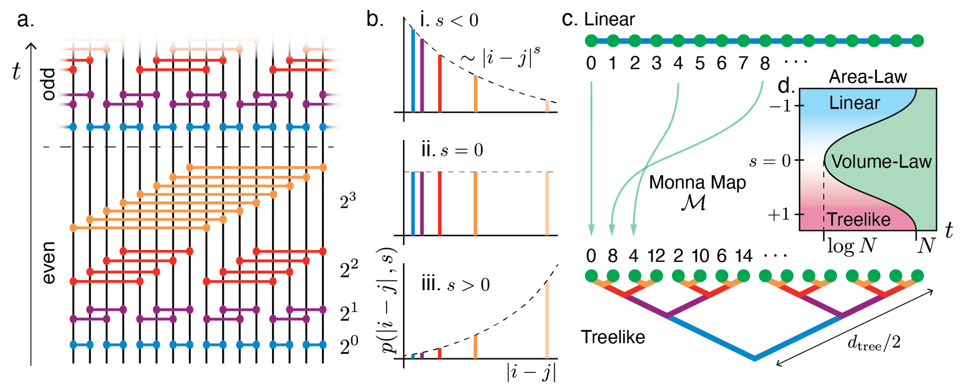
2. Sparse Clifford Circuits

In this paper, we study Clifford circuit models featuring sparse nonlocal interactions, where spin-1/2 qubits residing at sites $i,j=0,\dots ,N-1$ of a 1d chain interact if and only if they are separated by an integer power of 2: $\left|i-j\right|=2^{m-1}$ for $m=1,\dots ,{log}_{2}N$ (Figure 1a). A tunable parameter s controls how these couplings either decay ($s<0$) or grow ($s>0$) with distance as illustrated in Figure 1b. Recent analytical [30,31], numerical [29,32], and experimental [28] work has demonstrated that sparse nonlocal models of this type exhibit a transition in geometry as a function of the exponent s, yielding a linear (Euclidean) geometry for $s<0$, a treelike (Ultrametric) geometry for $s>0$, and a fast-scrambling geometry at the midpoint $s=0$ between the two. These previous analyses [28,29,30,31,32] have argued that the flow of quantum information in such systems is governed by a linear lightcone when $s<0$ and by a treelike lightcone when $s>0$, and that both of these lightcones break down near $s=0$, allowing for fast scrambling dynamics.

Here we study the emergence of similar lightcones in analogous stochastic Clifford circuits. We use Clifford circuits in particular because they can be efficiently classically simulated [42,43] (Appendix A), while also capturing many-body entanglement. The dynamics of Clifford circuits closely mirror the dynamics of general random unitary circuits [9,44] because Clifford circuits are unitary 2-designs [45]. Our circuits are composed of random two-qubit Clifford gates $Q_{ij}=Q_{ji}$, where the exponent s controls the probability $p(\left|i-j\right|,s)$ of placing a gate $Q_{ij}$ between qubits $i,j$ during each timestep $\delta t$. In the sparse Clifford circuit, the gates are arranged in a nonlocal bricklayer pattern illustrated in Figure 1a, with interaction layers stacked into an alternating sequence of ‘even’ and ‘odd’ blocks. During the ‘even’ block, a gate $Q_{ij}$ is placed between qubits $i<j$ with probability $p(\left|i-j\right|,s)$ if and only if $\mathrm{mod}(\lfloor i/2^{m-1}\rfloor ,2)=0$. During the subsequent odd block, gates are placed according to the same rules but with the odd-bricklayer condition $\mathrm{mod}(\lfloor i/2^{m-1}\rfloor ,2)=1$ [46]. Throughout the paper a single timestep $\delta t$ corresponds to applying a single even block followed by a single odd block. The probability of placing each gate $Q_{ij}$ is modulated according to the sparse probability distribution

$$p(\left|i-j\right|,s)=\left\{\begin{array}{cc}{J}_s{\left|i-j\right|}^s\hfill & \mathrm{when}\left|i-j\right|=2^{m-1}\hfill \\ 0\hfill & \mathrm{otherwise}\hfill \end{array}\right.$$

(1)

which mimics the sparse coupling matrix $J(\left|i-j\right|,s)$ used in analogous continuous-time models [29]. The normalization factor $J_s$ ensures that one gate, on average, is applied per site during each timestep $\delta t$ (see Appendix B). Thus, short-distance gates dominate the Clifford circuit when $s<0$ while long-distance gates dominate when $s>0$ (Figure 1b top and bottom). At the midpoint $s=0$, gates at all length scales are equally probable in the circuit (Figure 1b middle). Here and throughout the paper, we impose periodic boundary conditions, such that the linear distance $\left|i-j\right|$ between a pair of sites is the smaller of $\mathrm{abs}(i-j)$ and $N-\mathrm{abs}(i-j)$.

3. Probing Emergent Geometry with Entanglement Entropy

We begin characterizing the geometry generated by the circuit by examining the pattern of entanglement present in various subregions A of the output qubits as illustrated in Figure 2a. Because the circuit is composed entirely of Clifford gates, we may completely characterize the entanglement in the system at any time t by computing Renyi entropies $S_A\equiv S_A^{\left(2\right)}=-lnTr\left[{\rho }_A^2\right]$ of subregions A [43,47]. In this section, we study Renyi entropies of contiguous subregions A, where the meaning of the word ‘contiguous’ depends on the geometry implied by the interactions. A linearly-contiguous region A has the property that any bipartition $A=A_1\bigcup A_2$ is contiguous with respect to the Euclidean metric: for every $i\in A_1$, there exists a $j\in A_2$ such that $\left|i-j\right|=1$. When $s<0$, we shall find that the entanglement generated by the circuit is organized into linearly-contiguous subregions.

By contrast, in the limit $s>0$, we shall find that the entanglement in the circuit is organized into treelike-contiguous regions defined by the treelike (2-adic) metric ${\left|i-j\right|}_2=2^{d_{tree}(i,j)/2}/N$, where $d_{tree}(i,j)$ is the number of edges required to connect sites i and j in the regular binary tree shown at the bottom of Figure 1c (see Appendix C for a more comprehensive discussion of the 2-adic metric ${\left|i-j\right|}_2$). A treelike-contiguous region A is defined by the property that any bipartition $A=A_1\bigcup A_2$ is contiguous with respect to the treelike (2-adic) metric: for every $i\in A_1$, there exists a $j\in A_2$ such that ${\left|i-j\right|}_2=2/N$ for N a power of 2. One can obtain the sites $i,j$ in the treelike ordering by rearranging the qubits by the discrete Monna map $\mathcal{M}$, which reverses the digits of the argument when written in base 2 (c.f. Appendix C). For example, in a system with $N=8$ qubits, site 1 is mapped to site $\mathcal{M}\left(1\right)=4$ under the Monna map because $\mathcal{M}\left({001}_2\right)={100}_2$ when the site numbers are written in binary.

Simply relabeling the sites under the Monna map $\mathcal{M}$ is not enough to constitute a distinct geometry, but the treelike structure of the 2-adic metric ${\left|i-j\right|}_2$ endows this arrangement with a notion of distance that is entirely different from the conventional metric $\left|i-j\right|$ in linear (Euclidean) geometry. Specifically, while both measures of distance satisfy the usual mathematical axioms required for a metric, the 2-adic measure is ultrametric, meaning that it satisfies a much stronger form of the triangle inequality ${\left|i-j\right|}_2\le \max ({\left|i-k\right|}_2,{\left|j-k\right|}_2)$ for all $i,j,k$. Additionally, while both geometries are translation-invariant $(i,j)\to (i+\ell ,j+\ell )modN$, the treelike geometry is also invariant under a much larger number of nested permutation symmetries which exchange the left and right halves of any subtree. In particular, by consecutively applying exchange permutations at each level of the tree in Figure 1c we obtain translational invariance in the treelike geometry, i.e., $d_{tree}(i+1,j+1)=d_{tree}(i,j)$ [17,18,48,49,50,51].

Inspired by the growth of entanglement in lattice systems, we expect typical contiguous subregions A of output qubits to be volume-law entangled $S_A\sim \left|A\right|$ when they are small enough to lie entirely inside the system’s many-body lightcone, but to cross over to area-law entanglement $S_A\sim \mathrm{const}.$ when the region becomes much larger than the extent of the lightcone at a given time, as illustrated in Figure 2a. On the contrary, geometrically disjoint subregions—for example, arbitrary subsets of $k\ll N$ qubits chosen at random from anywhere in the system—typically exhibit volume-law entanglement after only a single layer of gates, which originates trivially from the short-range entanglement in the system. This distinction between area-law and volume-law scaling in the entanglement entropy therefore provides a simple and sharp test of geometrical contiguity. Specifically, contiguous subregions A should exhibit area-law entanglement scaling at short times, whereas non-contiguous subregions should exhibit volume-law scaling.

We therefore proceed to use the scaling of the Renyi entropy with subregion $\left|A\right|$ as a quantitative probe of the system’s geometry. This is clearly illustrated in Figure 2, where we analyze the growth of entanglement in the sparse Clifford circuit acting on qubits initialized in a product state ${\left|0\right.〉}^{⨂N}$, where $\left|0\right.〉$ is the ground state of the Pauli-Z operator. The colour shading in Figure 2a shows the entanglement entropy $S_A$ of contiguous subregions A as a function of their size $\left|A\right|$ and time t with either linearly-contiguous bipartitions (top) or treelike-contiguous bipartitions (bottom). Taking a time-slice $t=6$ from Figure 2a, we find area-law scaling in the linear geometry at negative values of $s<0$ (Figure 2b, left), whereas other choices of geometry yield volume-law entanglement. Similarly, at positive values of $s>0$ we find area-law scaling in the treelike geometry and volume-law entanglement for other choices of geometry (Figure 2b, right). The non-monotonic features appearing at early times in Figure 2b are a direct result of the treelike geometric structure present in the circuit at large $s>0$. For instance, a treelike region consisting of precisely half the qubits $\left|A\right|=N/2$ has especially low entropy at early times coming from the weakest long-range interactions in the deepest parts of the tree (blue couplings in Figure 1c). By contrast, smaller treelike regions $\left|A\right|<N/2$ will have additional entropy coming from couplings higher in the tree (purple, red, orange in Figure 1c). Together, these observations confirm that the entanglement entropy has a volume-law scaling for typical regions A and an area-law scaling $S_A\sim O\left(1\right)$ when the regions are chosen to be either linearly- or treelike-contiguous depending on the value of s.

Finally, we estimate the timescale $t_{\mathrm{vol}.}$ required for extensive contiguous regions $\left|A\right|=N/2$ to saturate to volume-law entanglement. In the linear regime $s<0$, we find that this timescale grows linearly in the system size $t_{\mathrm{vol}.}\sim N$. In the treelike regime $s>0$, on the other hand, we find that this timescale grows polynomially in the system size $t_{\mathrm{vol}.}\sim N^{\left|s\right|}$ (Appendix D). This is expected because the local geometry in each case inhibits the spreading of quantum information through the system, and an extensive subregion A cannot become volume-law entangled until the lightcone of a single qubit has spread to of order $\left|A\right|$ qubits [38]. By contrast, near the crossover point $s=0$ the circuit achieves volume-law entanglement on much shorter timescales consistent with logarithmic scaling $t_{\mathrm{vol}.}\sim lnN$, which indicates fast scrambling dynamics [29,32,37,40,52,53,54,55,56].

4. Scrambling and Negativity of Tripartite Mutual Information

In the previous section we observed that local lightcones in the linear and treelike regimes prevent the buildup of system-wide entanglement until times of order $t\sim \mathcal{O}\left(N\right)$. We can more precisely study the growth of these correlations by considering the scrambling of quantum information as diagnosed by the tripartite mutual information

$$\begin{array}{c}\hfill I(A:B:C)=I(A;B)+I(A;C)-I(A;BC)\end{array}$$

(2)

of three geometrically contiguous subregions $A,B,C$ of equal size $N/4$, where $I(A;B)=S_A+S_B-S_{AB}$ is the mutual information between regions A and B. The tripartite mutual information vanishes when the regions are uncorrelated, but becomes negative $I(A:B:C)<0$ as entanglement builds up across the system [57,58,59]. Negativity of the tripartite mutual information for three extensive regions $A,B,C$ therefore serves as a natural measure of the degree to which nonlocal correlations have built up across the entire system.

In our sparse Clifford circuits, we find that the time dependence of the tripartite mutual information varies dramatically depending on the value of s as shown in Figure 3a. For large $\left|s\right|>1$, the locality of the interactions in both the linear and treelike geometries results in an effective lightcone that prevents system-wide scrambling at short times, which appears in Figure 3a as a long plateau near $I(A:B:C)=0$. Only after timescales extensive in N, when the local lightcone has spread to cover the entire system, do we observe appreciable negativity in the tripartite mutual information. Near $\left|s\right|=0$, by contrast, the tripartite mutual information becomes negative in a timescale of order $t_{*}\sim \mathcal{O}\left(1\right)$ due to the emerging hierarchical structure of the circuit (see Appendix F). At long times the tripartite mutual information approaches the expected steady-state value of $I(A:B:C)\approx -\frac{N}{2}ln2$ (Appendix G).

We can quantitatively extract the timescale required for system-wide entanglement to build up in our circuits by computing the time $t_0$ required to reach one bit of negativity in the tripartite mutual information in a given geometry. With qubits arranged in a conventional linear geometry (Figure 3a left, orange), this timescale grows as $t_0^{\mathrm{linear}}\sim N$ for $s<-1$ for large system sizes. In the treelike geometry, for $1<s$ the time $t_0^{\mathrm{treelike}}$ grows like $t_0^{max}\sim N^{\beta }$ with $\beta \sim s+0.1$ (Figure 3a right, red). Finally, at the crossover point $s=0$ we find that $t_0^{max}=max\{t_0^{\mathrm{linear}},t_0^{\mathrm{treelike}}\}$ converges towards $t=1$ as shown in Figure 3b (see Appendix F for further details and discussion). This quick loss of locality of the interactions in the two mathematically incompatible geometries near $s=0$ further confirms the fast-scrambling nature of this circuit.

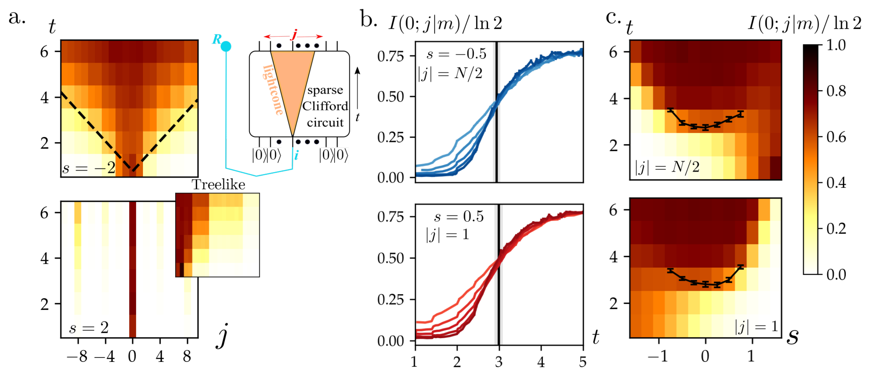
5. Characterizing the Many-Body Lightcone via Teleportation

One can obtain a striking picture of the system’s local geometry by studying its lightcone, which governs the propagation of quantum information in general quantum systems [29,33,34,38]. In 1 + 1d systems with local interactions this lightcone is linear, such that information can reliably propagate between spatially separated sites $i,j$ only if they lie inside the lightcone $\left|i-j\right|<v_{s}t$ for some finite velocity $v_s$. The velocity $v_s$ is sometimes called the Lieb–Robinson velocity or the butterfly velocity depending on context, and its numerical value depends on the microscopic details of the system. Previous work has studied lightcones in tunable sparse models using free-fermion and MPS numerics [29] as well as via field-theory methods [30,31]. In particular, these previous results indicated the emergence of a linear lightcone $\left|i-j\right|<v_{s}t$ for sufficiently negative $s<0$ and a treelike lightcone ${\left|i-j\right|}_2<v_{s}t$ characterized by the treelike 2-adic distance ${\left|·\right|}_2$ for sufficiently positive $s>0$. Here we present evidence for similar emergent lightcones in our family of sparse Clifford circuits, which allows us to probe the linear-treelike transition in the strongly-interacting limit.

To probe the many-body lightcone, we ask whether it is possible to teleport a single qubit of information from a particular location i at the input of the circuit to another location j at the output [60] as illustrated in Figure 4a. Teleportation via the standard Hayden–Preskill–Yoshida–Kitaev mechanism succeeds when the input is strongly scrambled into an output region containing the output qubit j [61,62,63]. We therefore expect teleportation to succeed inside the lightcone $\left|i-j\right|<v_{s}t$ and to fail outside of it. To test this in our tunable Clifford circuits, we maximally entangle a single reference qubit R with the input qubit i as illustrated in Figure 4a. We then measure the mutual information

$$I(i;j|m)=\left(S_i+S_j-S_{ij}\right){|}_m$$

(3)

between the input and output qubit j, conditioned on performing projective measurements in the Pauli-Z basis on all qubits except qubits $R,j$ [60].

When $s<0$ this procedure yields a linear lightcone at short times, as shown in Figure 4a (black dashed), with a velocity $v_s\approx 3.0$. By contrast, when $s>0$ this lightcone is apparently destroyed, and information can teleport between distantly-separated sites $i,j$ only when they are separated by large powers of 2. Upon rearranging the sites by the Monna map, however, we recover a treelike lightcone as measured by the treelike 2-adic distance ${\left|i-j\right|}_2<v_{s}t$ (inset). These emergent lightcones demonstrate that our circuits behave locally for large $\left|s\right|$, but that the notion of locality depends strongly on the sign of s, yielding local dynamics in either conventional linear geometry when $s<0$ or treelike geometry when $s>0$.

Near the crossover point $s=0$ between these two geometries, we expect both local lightcones to collapse, yielding fast scrambling dynamics where information rapidly spreads throughout the system [29]. These fast-scrambling dynamics should exhibit a finite-time teleportation phase transition similar to that found recently in all-to-all random circuits [60]. We study this phase transition as a function of $-1<s<1$ in Figure 4c, using pairs of qubits $i,j$ that are either maximally separated in linear distance $\left|i-j\right|=N/2$ (top) or maximally separated in treelike distance ${\left|i-j\right|}_2=1$ (bottom). Both choices yield a clear phase transition at a critical time $t_c\left(s\right)$ for circuits near $s=0$. The critical time $t_c\left(s\right)$ is extracted at each value of s by determining the crossing point of the teleportation fidelity at early times in a finite-size scaling analysis (Figure 4b). These critical points are overlaid in black on Figure 4c. By contrast, similar finite-size scaling analysis in the local regimes $1\le \left|s\right|$ yield no such crossings, indicating that there is no longer a finite-time phase transition in these regimes. Together, these results provide clear evidence of emergent lightcones in the linear $s<0$ and treelike $s>0$ regimes, separated by the nonlocal regime characterized by a finite-teleportation-time facilitated by the fast scrambling dynamics near $s=0$.

6. Conclusions and Outlook

In this paper, we studied tunable effective geometries that emerge in sparse circuits, using Clifford circuits as toy models. To characterize the effective geometries in these circuits we numerically computed Renyi entropies of contiguous regions of output qubits A as a function of time, where the term ‘contiguous’ was defined either according to the linear (Euclidean) metric $\left|i-j\right|$ or according to the treelike 2-adic metric ${\left|i-j\right|}_2$. In Section 3, we found area-law entanglement at short times $t<N$ in both of the local regimes $\left|s\right|>1$, indicating linear entanglement growth for negative $s<0$ and treelike entanglement growth in a treelike geometry for positive $s>0$. We confirmed these findings in Section 4 where we studied the timescale for quantum information to become scrambled as quantified by the negativity of the tripartite mutual information $I(A:B:C)$. There we found that either a linear ($s<0$) or treelike ($s>0$) lightcone prevents system-wide scrambling earlier than a time $t_0\sim \mathcal{O}\left(N^a\right)$ in the local regimes $\left|s\right|>1$. Finally, in Section 5 we explicitly mapped the system’s many-body lightcone by considering the fidelity $I(i;j|m)$ of teleporting a single qubit of information from an input qubit i to an output qubit j. Here we found that teleportation succeeds if the ouput qubit j resides inside the many-body lightcone of the intput qubit i, and fails if j lies outside this lightcone. We demonstrated that this lightcone has a linear structure for $s<0$ and a treelike structure for $s>0$. Near the crossover point $s=0$ both of these lightcones collapse and teleportation succeeds in a finite time $t_c\left(s\right)$ that depends on the exponent s.

While in this work we were able to extract the teleportation time $t_c\left(s\right)$ for $-1<s<1$ in finite-size scaling analysis, future work may explore how this phase disintegrates near $\left|s\right| = 1$, where the teleportation time diverges in the thermodynamic limit. Using the teleportation time $t_c\left(s\right)$ as a diagnostic, one might expect to observe a phase transition from a fast scrambling phase to a slow scrambling phase as a function of the parameter s near the points $\left|s\right| = 1$. It would also be interesting to study similar questions in Brownian qubit or fermion models, where analytical results are often possible [64,65]. In particular, these Brownian models typically lead to a description of entanglement dynamics in terms of effective field theories. Defining one of these theories on a sparse coupling graph such as the one considered here might allow us to make contact between the entanglement dynamics studied here and analytical field-theory approaches [30].

References

1. Gioev, D.; Klich, I. Entanglement Entropy of Fermions in Any Dimension and the Widom Conjecture. Phys. Rev. Lett. 2006, 96, 100503. [Google Scholar] [CrossRef] [Green Version]
2. Wolf, M.M. Violation of the Entropic Area Law for Fermions. Phys. Rev. Lett. 2006, 96, 010404. [Google Scholar] [CrossRef] [Green Version]
3. Hastings, M.B.; Koma, T. Spectral Gap and Exponential Decay of Correlations. Commun. Math. Phys. 2006, 265, 781–804. [Google Scholar] [CrossRef] [Green Version]
4. Vidal, G. Entanglement Renormalization. Phys. Rev. Lett. 2007, 99, 220405. [Google Scholar] [CrossRef] [PubMed] [Green Version]
5. Hastings, M.B. An area law for one-dimensional quantum systems. J. Stat. Mech. Theory Exp. 2007, 2007, P08024. [Google Scholar] [CrossRef]
6. Eisert, J.; Cramer, M.; Plenio, M.B. Colloquium: Area laws for the entanglement entropy. Rev. Mod. Phys. 2010, 82, 277–306. [Google Scholar] [CrossRef] [Green Version]
7. Bianchi, E.; Hackl, L.; Kieburg, M.; Rigol, M.; Vidmar, L. Volume-Law Entanglement Entropy of Typical Pure Quantum States. arXiv 2021, arXiv:2112.06959. [Google Scholar]
8. Nahum, A.; Ruhman, J.; Vijay, S.; Haah, J. Quantum Entanglement Growth under Random Unitary Dynamics. Phys. Rev. X 2017, 7, 031016. [Google Scholar] [CrossRef] [Green Version]
9. Nahum, A.; Vijay, S.; Haah, J. Operator Spreading in Random Unitary Circuits. Phys. Rev. X 2018, 8, 021014. [Google Scholar] [CrossRef] [Green Version]
10. Skinner, B.; Ruhman, J.; Nahum, A. Measurement-Induced Phase Transitions in the Dynamics of Entanglement. Phys. Rev. X 2019, 9, 31009. [Google Scholar] [CrossRef] [Green Version]
11. Li, Y.; Fisher, M.P. Statistical mechanics of quantum error correcting codes. Phys. Rev. B 2021, 103, 104306. [Google Scholar] [CrossRef]
12. Maldacena, J. The large-N limit of superconformal field theories and supergravity. Int. J. Theor. Phys. 1999, 38, 1113–1133. [Google Scholar] [CrossRef] [Green Version]
13. Gubser, S.S.; Klebanov, I.R.; Polyakov, A.M. Gauge theory correlators from non-critical string theory. Phys. Lett. B 1998, 428, 105–114. [Google Scholar] [CrossRef] [Green Version]
14. Witten, E. Anti de Sitter space and holography. arXiv 1998, arXiv:hep-th/9802150. [Google Scholar] [CrossRef]
15. Hartnoll, S.A. Lectures on holographic methods for condensed matter physics. Class. Quantum Gravity 2009, 26, 224002. [Google Scholar] [CrossRef] [Green Version]
16. Swingle, B. Entanglement renormalization and holography. Phys. Rev. D 2012, 86, 065007. [Google Scholar] [CrossRef]
17. Gubser, S.S.; Knaute, J.; Parikh, S.; Samberg, A.; Witaszczyk, P. p-Adic AdS/CFT. Commun. Math. Phys. 2017, 352, 1019–1059. [Google Scholar] [CrossRef] [Green Version]
18. Heydeman, M.; Marcolli, M.; Saberi, I.; Stoica, B. Tensor networks, p-adic fields, and algebraic curves: Arithmetic and the AdS3/CFT2 correspondence. arXiv 2017, arXiv:hep-th/1605.07639. [Google Scholar]
19. Ryu, S.; Takayanagi, T. Holographic Derivation of Entanglement Entropy from the anti–de Sitter Space/Conformal Field Theory Correspondence. Phys. Rev. Lett. 2006, 96, 181602. [Google Scholar] [CrossRef] [Green Version]
20. Ryu, S.; Takayanagi, T. Aspects of holographic entanglement entropy. J. High Energy Phys. 2006, 2006, 045. [Google Scholar] [CrossRef] [Green Version]
21. Hubeny, V.E.; Rangamani, M.; Takayanagi, T. A covariant holographic entanglement entropy proposal. J. High Energy Phys. 2007, 2007, 62. [Google Scholar] [CrossRef]
22. Islam, R.; Ma, R.; Preiss, P.M.; Eric Tai, M.; Lukin, A.; Rispoli, M.; Greiner, M. Measuring entanglement entropy in a quantum many-body system. Nature 2015, 528, 77–83. [Google Scholar] [CrossRef] [PubMed]
23. Hucul, D.; Inlek, I.V.; Vittorini, G.; Crocker, C.; Debnath, S.; Clark, S.M.; Monroe, C. Modular entanglement of atomic qubits using photons and phonons. Nat. Phys. 2015, 11, 37–42. [Google Scholar] [CrossRef] [Green Version]
24. Kaufman, A.M.; Tai, M.E.; Lukin, A.; Rispoli, M.; Schittko, R.; Preiss, P.M.; Greiner, M. Quantum thermalization through entanglement in an isolated many-body system. Science 2016, 353, 794–800. [Google Scholar] [CrossRef] [PubMed] [Green Version]
25. Hosten, O.; Engelsen, N.J.; Krishnakumar, R.; Kasevich, M.A. Measurement noise 100 times lower than the quantum-projection limit using entangled atoms. Nature 2016, 529, 505–508. [Google Scholar] [CrossRef] [PubMed]
26. Lukin, A.; Rispoli, M.; Schittko, R.; Tai, M.E.; Kaufman, A.M.; Choi, S.; Khemani, V.; Léonard, J.; Greiner, M. Probing entanglement in a many-body–localized system. Science 2019, 364, 256–260. [Google Scholar] [CrossRef]
27. Brydges, T.; Elben, A.; Jurcevic, P.; Vermersch, B.; Maier, C.; Lanyon, B.P.; Zoller, P.; Blatt, R.; Roos, C.F. Probing Renyi entanglement entropy via randomized measurements. Science 2019, 364, 260–263. [Google Scholar] [CrossRef] [Green Version]
28. Periwal, A.; Cooper, E.S.; Kunkel, P.; Wienand, J.F.; Davis, E.J.; Schleier-Smith, M. Programmable interactions and emergent geometry in an array of atom clouds. Nature 2021, 600, 630–635. [Google Scholar] [CrossRef]
29. Bentsen, G.; Hashizume, T.; Buyskikh, A.S.; Davis, E.J.; Daley, A.J.; Gubser, S.S.; Schleier-Smith, M. Treelike Interactions and Fast Scrambling with Cold Atoms. Phys. Rev. Lett. 2019, 123, 130601. [Google Scholar] [CrossRef] [Green Version]
30. Gubser, S.S.; Jepsen, C.; Ji, Z.; Trundy, B. Continuum limits of sparse coupling patterns. Phys. Rev. D 2018, 98, 045009. [Google Scholar] [CrossRef] [Green Version]
31. Gubser, S.S.; Jepsen, C.; Ji, Z.; Trundy, B. Mixed field theory. J. High Energ. Phys. 2019, 2019, 136. [Google Scholar] [CrossRef] [Green Version]
32. Hashizume, T.; Bentsen, G.S.; Weber, S.; Daley, A.J. Deterministic Fast Scrambling with Neutral Atom Arrays. Phys. Rev. Lett. 2021, 126, 200603. [Google Scholar] [CrossRef] [PubMed]
33. Lieb, E.H.; Robinson, D.W. The finite group velocity of quantum spin systems. Commun. Math. Phys. 1972, 28, 251–257. [Google Scholar] [CrossRef]
34. Hastings, M.B. Locality in quantum systems. Quantum Theory Small Large Scales 2010, 95, 171–212. [Google Scholar]
35. Roberts, D.A.; Swingle, B. Lieb–Robinson Bound and the Butterfly Effect in Quantum Field Theories. Phys. Rev. Lett. 2016, 117, 091602. [Google Scholar] [CrossRef] [Green Version]
36. Else, D.V.; Machado, F.; Nayak, C.; Yao, N.Y. Improved Lieb–Robinson bound for many-body Hamiltonians with power-law interactions. Phys. Rev. A 2020, 101, 022333. [Google Scholar] [CrossRef] [Green Version]
37. Bentsen, G.; Gu, Y.; Lucas, A. Fast scrambling on sparse graphs. Proc. Natl. Acad. Sci. USA 2019, 116, 6689–6694. [Google Scholar] [CrossRef] [Green Version]
38. Tran, M.C.; Guo, A.Y.; Baldwin, C.L.; Ehrenberg, A.; Gorshkov, A.V.; Lucas, A. Lieb-Robinson Light Cone for Power-Law Interactions. Phys. Rev. Lett. 2021, 127, 160401. [Google Scholar] [CrossRef]
39. Page, D.N. Average entropy of a subsystem. Phys. Rev. Lett. 1993, 71, 1291–1294. [Google Scholar] [CrossRef] [Green Version]
40. Sekino, Y.; Susskind, L. Fast scramblers. J. High Energy Phys. 2008, 2008, 065. [Google Scholar] [CrossRef] [Green Version]
41. Rammal, R.; Toulouse, G.; Virasoro, M.A. Ultrametricity for Physicists. Rev. Mod. Phys. 1986, 58, 765–788. [Google Scholar] [CrossRef]
42. Gottesman, D. The Heisenberg representation of quantum computers. arXiv 1998, arXiv:quant-ph/9807006. [Google Scholar]
43. Aaronson, S.; Gottesman, D. Improved simulation of stabilizer circuits. Phys. Rev. A 2004, 70, 052328. [Google Scholar] [CrossRef] [Green Version]
44. Li, Y.; Chen, X.; Fisher, M.P.A. Measurement-Driven Entanglement Transition in Hybrid Quantum Circuits. Phys. Rev. B 2019, 100, 134306. [Google Scholar] [CrossRef] [Green Version]
45. Cleve, R.; Leung, D.; Liu, L.; Wang, C. Near-Linear Constructions of Exact Unitary 2-Designs. Quantum Inf. Comput. 2016, 16, 721–756. [Google Scholar] [CrossRef]
46. Hashizume, T.; Bentsen, G.; Daley, A.J. Measurement-induced phase transitions in sparse nonlocal scramblers. arXiv 2021, arXiv:2109.10944. [Google Scholar] [CrossRef]
47. Rényi, A. On measures of entropy and information. In Proceedings of the Fourth Berkeley Symposium on Mathematical Statistics and Probability, Volume 1: Contributions to the Theory of Statistics; University of California Press: Berkeley, CA, USA, 1961; Volume 4, pp. 547–562. [Google Scholar]
48. Huang, A.; Stoica, B.; Yau, S.T. General relativity from p-adic strings. arXiv 2021, arXiv:1901.02013. [Google Scholar]
49. Stoica, B. Building Archimedean Space. arXiv 2021, arXiv:1809.01165. [Google Scholar]
50. Gubser, S.S.; Heydeman, M.; Jepsen, C.; Marcolli, M.; Parikh, S.; Saberi, I.; Stoica, B.; Trundy, B. Edge length dynamics on graphs with applications to p-adic AdS/CFT. J. High Energ. Phys. 2017, 2017, 157. [Google Scholar] [CrossRef]
51. Bentsen, G.S.; Hashizume, T.; Davis, E.J.; Buyskikh, A.S.; Schleier-Smith, M.H.; Daley, A.J. Tunable geometries from a sparse quantum spin network. In Proceedings of the Optical, Opto-Atomic, and Entanglement-Enhanced Precision Metrology II; International Society for Optics and Photonics: Bellingham, WA, USA, 2020; Volume 11296, p. 112963W. [Google Scholar]
52. Lashkari, N.; Stanford, D.; Hastings, M.; Osborne, T.; Hayden, P. Towards the fast scrambling conjecture. J. High Energ. Phys. 2013, 2013, 22. [Google Scholar] [CrossRef] [Green Version]
53. Yao, N.Y.; Grusdt, F.; Swingle, B.; Lukin, M.D.; Stamper-Kurn, D.M.; Moore, J.E.; Demler, E.A. Interferometric approach to probing fast scrambling. arXiv 2016, arXiv:1607.01801. [Google Scholar]
54. Marino, J.; Rey, A. Cavity-QED simulator of slow and fast scrambling. Phys. Rev. A 2019, 99, 051803(R). [Google Scholar] [CrossRef] [Green Version]
55. Li, Z.; Choudhury, S.; Liu, W.V. Fast scrambling without appealing to holographic duality. Phys. Rev. Res. 2020, 2, 043399. [Google Scholar] [CrossRef]
56. Belyansky, R.; Bienias, P.; Kharkov, Y.A.; Gorshkov, A.V.; Swingle, B. Minimal Model for Fast Scrambling. Phys. Rev. Lett. 2020, 125, 130601. [Google Scholar] [CrossRef] [PubMed]
57. Hayden, P.; Headrick, M.; Maloney, A. Holographic Mutual Information Is Monogamous. Phys. Rev. D 2013, 87, 046003. [Google Scholar] [CrossRef] [Green Version]
58. Hosur, P.; Qi, X.L.; Roberts, D.A.; Yoshida, B. Chaos in quantum channels. J. High Energy Phys. 2016, 2016, 4. [Google Scholar] [CrossRef] [Green Version]
59. Gullans, M.J.; Huse, D.A. Dynamical Purification Phase Transition Induced by Quantum Measurements. Phys. Rev. X 2020, 10, 041020. [Google Scholar] [CrossRef]
60. Bao, Y.; Block, M.; Altman, E. Finite time teleportation phase transition in random quantum circuits. arXiv 2021, arXiv:2110.06963. [Google Scholar]
61. Hayden, P.; Preskill, J. Black holes as mirrors: Quantum information in random subsystems. J. High Energy Phys. 2007, 2007, 120. [Google Scholar] [CrossRef] [Green Version]
62. Yoshida, B.; Kitaev, A. Efficient decoding for the Hayden-Preskill protocol. arXiv 2017, arXiv:1710.03363. [Google Scholar]
63. Yoshida, B.; Yao, N.Y. Disentangling Scrambling and Decoherence via Quantum Teleportation. Phys. Rev. X 2019, 9, 011006. [Google Scholar] [CrossRef] [Green Version]
64. Zhang, P.; Jian, S.K.; Liu, C.; Chen, X. Emergent Replica Conformal Symmetry in Non-Hermitian SYK _2 Chains. Quantum 2021, 5, 579. [Google Scholar] [CrossRef]
65. Bentsen, G.S.; Sahu, S.; Swingle, B. Measurement-induced purification in large-N hybrid Brownian circuits. Phys. Rev. B 2021, 104, 094304. [Google Scholar] [CrossRef]
66. Selinger, P. Generators and relations for n-qubit Clifford operators. Log. Meth. Comput. Sci. 2015, 11, 80–94. [Google Scholar] [CrossRef] [Green Version]
67. Nahum, A.; Roy, S.; Skinner, B.; Ruhman, J. Measurement and Entanglement Phase Transitions in All-To-All Quantum Circuits, on Quantum Trees, and in Landau-Ginsburg Theory. PRX Quantum 2021, 2, 010352. [Google Scholar] [CrossRef]
68. Gouvêa, F.Q. p-Adic Numbers, 3rd ed.; Springer: Cham, Switzerland, 1997. [Google Scholar]
69. Dyson, F.J. Existence of a Phase-Transition in a One-Dimensional Ising Ferromagnet. Commun. Math. Phys. 1969, 12, 91–107. [Google Scholar] [CrossRef]
70. Bleher, P.; Sinai, J. Investigation of the critical point in models of the type of Dyson’s hierarchical models. Commun. Math. Phys. 1973, 33, 23–42. [Google Scholar] [CrossRef]
71. Lerner, E.; Missarov, M. Scalar models of p-adic quantum field theory and hierarchical models. Theor. Math. Phys. 1989, 78, 177–184. [Google Scholar] [CrossRef]
72. Monna, A. Sur une transformation simple des nombres P-adiques en nombres reels. Indag. Math. (Proc.) 1952, 55, 1–9. [Google Scholar] [CrossRef]
73. Kolchin, V. Random Graphs; Encyclopedia of Mathematics and its Applications; Cambridge University Press: Cambridge, UK, 1998. [Google Scholar]
Figure 1. Sparse Clifford circuits yielding tunable geometries. Qubits i , j arranged in a linear chain interact pairwise (a) if and only if they are separated by a power of two, i j = 2 m 1 for m = 1 , 2 , , log 2 N . To mimic continuously-tunable interactions in a discrete circuit, we arrange random two-qubit gates into even and odd bricklayer blocks, and randomly apply each gate Q i j with probability p ( i j , s ) given in Equation (1). A tunable power-law exponent s (b) controls whether this distribution decays ( s < 0 , top) or grows ( s > 0 , bottom) with distance. The structure of entanglement generated by these circuits indicates linear (Euclidean) geometry when s < 0 and the treelike geometry of the 2-adic numbers when s > 0 (c). Numerical studies of entanglement entropies as a function of time reveal three distinct regimes (d): a linear area-law regime (blue) when s < 0 , a treelike area-law regime (red) when s > 0 , and a volume-law regime (green) at late times. In the two local regimes s > 1 , volume-law entanglement builds up on a timescale t * N that grows linearly with the system size, but near s = 0 fast scrambling dynamics generates volume-law entanglement on timescales as short as t * ln N .
Symmetry 14 00666 g001
Figure 2. Probing tunable geometry using entanglement entropy. (a) Entanglement growth in contiguous subregions A in a system of N = 64 qubits initialized in the product state 0 N , plotted as a function of subregion size A and time t in linear (top) and treelike (bottom) geometries. (b) A time-slice at t = 6 from the color-map illustrates the area-law scaling and volume-law scaling for linear (left) and treelike (right) geometries. When s < 0 , linearly contiguous subregions A exhibit area-law entanglement at short times, while other subregions are trivially volume-law entangled. When s > 0 , treelike subregions have area-law entanglement at short times, while other regions are volume-law entangled. (c) The timescale t vol . required to reach volume-law entanglement grows polynomially with system size N = 2 3 , , 2 7 when s > 1 , but is much shorter near s = 0 , consistent with a logarithmic scrambling time t vol . ln N . Error bars are shown or are smaller than data points. Data points are obtained by averaging over 10 2 trajectories.
Symmetry 14 00666 g002
Figure 3. Characterizing Scrambling using Tripartite Mutual Information. (a) The tripartite mutual information I ( A : B : C ) between three contiguous regions of size N / 4 (top left) of the output qubits for s = 1.5 , , 1.5 in steps of Δ s = 0.25 , in linear (left) and treelike (right) geometries for N = 512 . An initial plateau I ( A : B : C ) = 0 (white) persists for long times when the interactions are local in a given geometry. At long times, information eventually scrambles across the entire system, leading to substantial negativity (dark blue). We estimate the timescale of the initial plateau by finding the time t 0 required for the system to reach one bit of negativity I ( A : B : C ) = ln 2 when the regions A , B , C are chosen contiguously from either the linear (orange) or treelike (red) geometry. (b) The timescale t 0 for s = ± 0.0 , 0.4 , 0.7 , 1.5 grows rapidly with system size N in both of the local regimes s > 1 , but is insensitive to system size near the fast-scrambling limit s = 0 . Error bars are shown or are smaller than data points. Results are averaged over 10 3 circuit realizations with product state 0 N as the initial state (Appendix E).
Symmetry 14 00666 g003
Figure 4. Characterizing tunable geometry via teleportation. We probe the many-body lightcone in sparse Clifford circuits by maximally entangling a reference qubit with a fixed input qubit i and computing the mutual information I ( i ; j | m ) between the reference and a particular output qubit j as a function of distance i j (a). The mutual information characterizes the fidelity of teleporting a qubit from i to j, which is possible only after the input qubit i has been sufficiently scrambled into qubits lying inside the lightcone. When s = 1 we find a linear lightcone (top), where strong scrambling inside the lightcone (black dashed, v s 3.0 ) enables successful teleportation of quantum information from i to j. When s = 1 this lightcone is apparently destroyed (bottom), but a rearrangement of the sites by the Monna map M yields an emergent treelike lightcone as measured by the 2-adic distance i j 2 (inset). For 1 < s < 1 we find a finite-time phase transition (c) in the teleportation fidelity. To probe this phase transition for 1 < s 0 (top) we consider teleportation between qubits maximally separated in linear (Euclidean) distance i j = N / 2 ; for 0 s < + 1 (bottom) we consider qubits maximally separated in treelike 2-adic distance i j 2 = 1 . The critical points t c ( s ) of this transition are extracted at each s via finite-size scaling analysis (b) as explained in the main text. Error bars are shown in black.
Symmetry 14 00666 g004
Publisher’s Note: MDPI stays neutral with regard to jurisdictional claims in published maps and institutional affiliations.