Abstract
The paper presents a method of calculation of rotationally symmetric circular plates, supported on piles and having a stiffness changing in the radial direction. The method is based on the superposition rule, i.e., an initial plate supported on piles is treated as a combination of two plates clamped on a middle post with a small diameter, wherein the first plate is loaded such as the initial one and the second plate is loaded by forces occurring as reactions in the piles of the initial plate. Obtained results are concordant with the engineer’s intuition and a comparison of results for various plates shows high similarity between each other. As works dealing with the analogical problems have not been found in the literature, then this concordance and similarity can be acknowledged as a premise showing a correctness of the presented method. The results obtained in the method have been compared to results obtained in a professional FEM-based environment for building construction design. It has been stated that in many cases the results of the presented method are highly concordant to those of the FEM, though in some cases discrepancies exist. However, the FEM is an approximate method, especially if related to plates, thus its results should be taken with a great care. In general, it can be stated that the presented method deserves an attention and further studies.
1. Introduction
The piles are a type of the direct foundation. Plates resting on piles as building elements find wide application, especially in constructions settled on wetlands and permafrost. It is common to build plates on piles as drilling platforms on seas as well as viewing terraces on seashores and lakes or on marshes close to the shores.
Rotationally symmetric circular plates, subjected to axisymmetric loading, are such a type of plates for which it is possible to find exact analytical solutions [1]. For rectangular plates, the more for otherwise shaped plates, it will be only approximate solutions (often in a form of infinite trigonometric series, usually numerical). Theory of plates, cooperating with a subsoil or without such cooperation, has been already well developed and a lot of problems has been well examined. The classical items concerning statics of plates are the books by Timoshenko [2] and Kączkowski [3], both of them republished several times, and of newer items it is worth to name a book by Blaauwendraad [4], comprising also a FEM analysis with reference to plates. Since then, many authors have dealt with circular plates on an elastic subsoil, both in terms of statics and dynamics as well as stability.
In recent years, an interest in elements with variable features has increased. Such elements give greater possibilities of shaping of a behavior of a construction and optimization of execution costs, e.g., by reduction of an element thickness in a place where it is subjected to a lower load. Due to that, methods should be developed which allow more effective calculation of such elements. The circular plates with variable features were also the subject of interest of many authors, wherein it is worth to cite the publications by Reddy [5,6], which treat of plates with functional gradation of features in the radial direction.
Another problem is a modelling of the cooperation of plates with piles and piles with a subsoil. Publications concerning this topic, however, do not refer to a behavior of plates settled on piles and elevated over a subsoil, i.e., not cooperating with a subsoil. All works found in the literature by the authors of this study concern the design of piles as well as behavior of plates on a subsoil reinforced by the piles. However, the plates described above, i.e., for example drilling or viewing platforms over the water and laid on piles put on a seabed, require calculations without consideration of the cooperation with subsoil (because there is no any), but with consideration of a point support in selected places. The authors were not able to find such publications.
Due to that, the task of this study is to calculate a deflection and internal forces (i.e., radial and tangential moments as well as radial shear forces) of a radially symmetric circular plate, supported in points (on piles) distributed on a circle (or circles) having a certain radius, in particular on a circumference. The term “radially symmetric” means that:
- the load and stiffness of the plate are axisymmetric, i.e., they are variable in the radial direction and constant in the tangent direction,
- the supports (piles) are evenly distributed, i.e., if straight sections are dragged from the center of the plate to each support, then between two such sections always exists a constant angle, even if the supports are distributed on the circles with different radii.
The main topic of the study are the plates with discontinuous (piecewise constant) stiffness, however the plates with functionally varying stiffness have been also examined as a comparison. The stiffness variability has been introduced through the thickness variability—the material itself is homogeneous. For the case of plates with discontinuous stiffness, the plate was approximated by homogeneous rings with different stiffnesses. Such approach was applied for example by Utku et al. [7]. It has been assumed as well, that one ring in such plate is wholly loaded or wholly unloaded on its surface—there is no situation where it is loaded only on a part of its surface. All plates have been calculated with use of the Kirchhoff’s theory of thin plates.
2. Materials and Methods
The plate presented in the Introduction can be calculated in two ways:
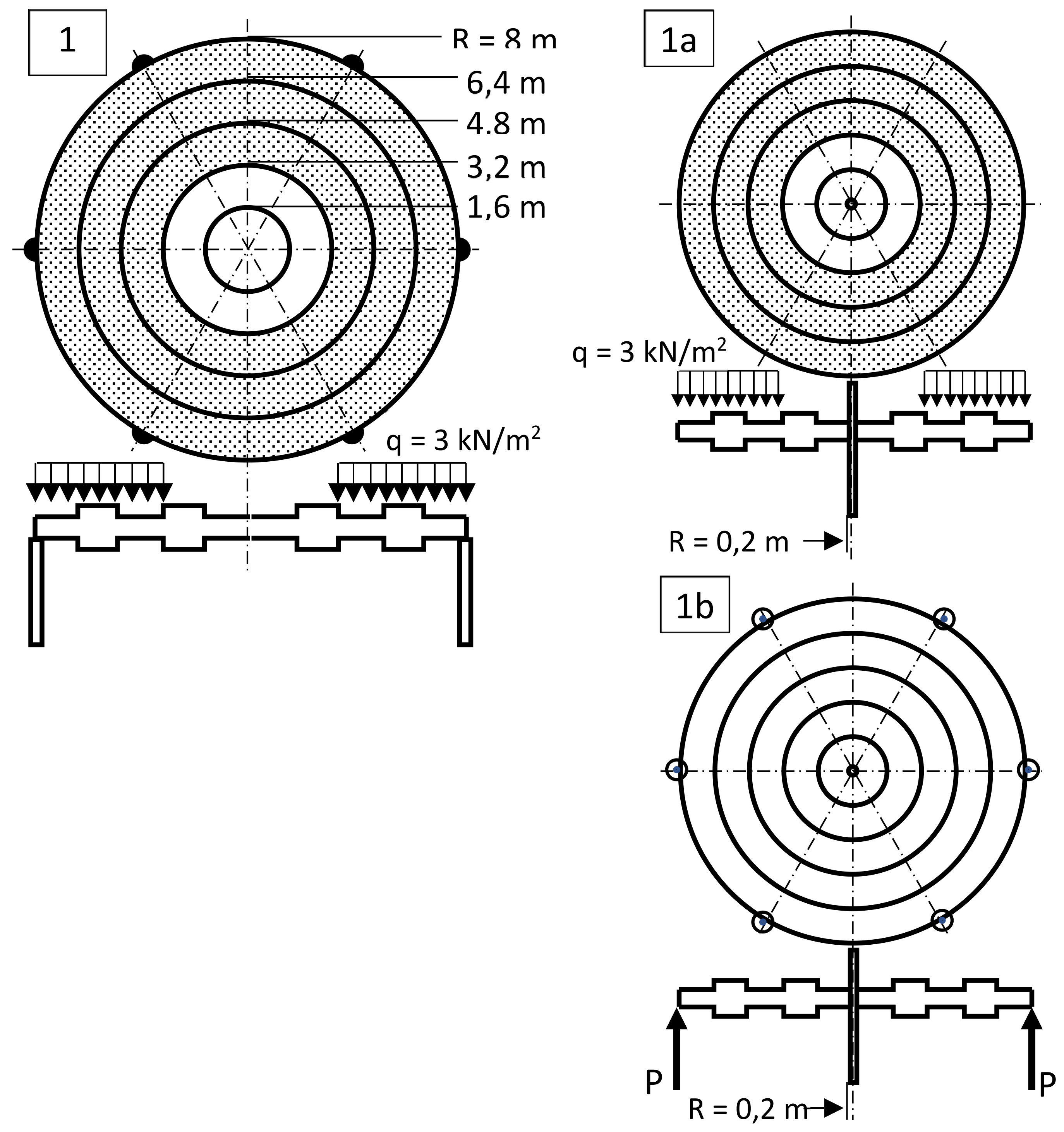
- using formulas for a plate on an elastic subsoil, wherein for the rings different than the external one, assuming a zero stiffness of subsoil and for the external ring a stiffness described by the “Dirac comb” (Figure 1a),
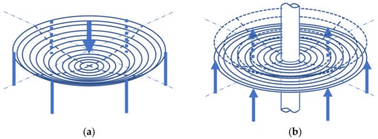 Figure 1. Possible approaches for calculation of rotationally symmetric plates settled on piles. (a) plate on external piles, (b) plate on an internal post.
 - treating the plate as supported around the middle on a small, defined radius (“supported” means clamped if there is no opening in the middle of the original plate or hinged if there is) and loaded by concentrated forces, in fact, being reactions to an external, real load (Figure 1b).
The first approach is much more difficult as the deflection of a circular plate on a subsoil requires a lot of complicated calculations (the formula contains the Bessel functions and functions related to them). Therefore, the second approach has been chosen.
According [2,3], the equation of deflection of a circular plate is following:
and the formulas for internal forces—following:
- radial bending moments:
- tangential bending moments:
- radial shear forces:
In the above formulas and further, w denotes deflection, q—surface load, r and —radial and angular coordinates, respectively, and —the plate stiffness: .
A solution to Equation (1) for a general case can be sought if the deflection and load are expanded into a cosine-sine series:
where,
i.e., it is assumed that the expansion occurs only in the tangential direction, wherein δ is the Kronecker symbol: δmn = 0 for m ≠ n and δmn = 1 for m = n.
If the deflection and load in the Formula (5) is substituted into Equation (1), then the differentiation with respect to r and φ will remain the cosine and sine without changes (only the expansion coefficient wm will be differentiated), moreover the differentiation with respect to φ—as it is always twice or fourfold—can change their sign and will cause their multiplication by m2 or m4:
Equation (7) will be satisfied if two separate equations are satisfied:
In general case, the complementary functions of these equations are following:
however, for m = 0 and m = 1 it is,
In Formulas (9) and (10) A0–D0 and Am–Dm are the integration constants, calculated from boundary and continuity conditions.
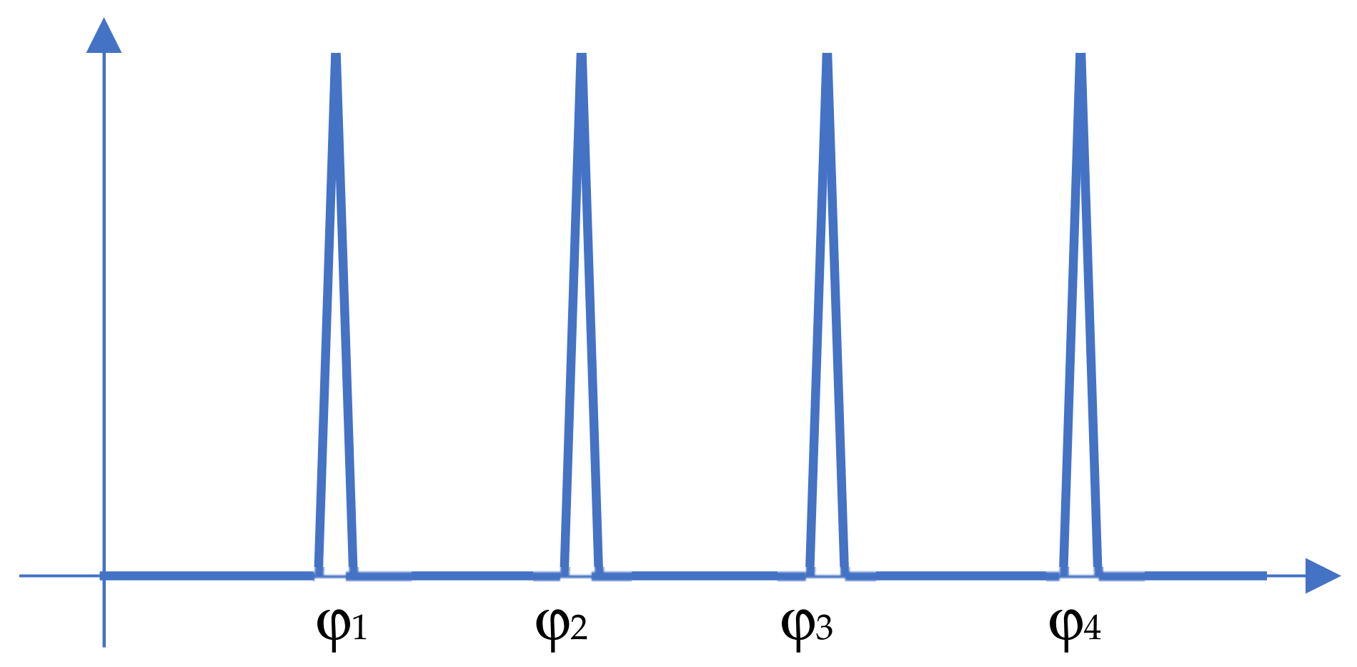
Assume a load in a form of several concentrated forces P, evenly distributed on circles having a certain radius (in particular, on a circumference) and summing in total to the real force in the middle. Such a load can be presented in the form of “Dirac comb” (Figure 2), i.e., the expression:
where n—the number of piles and the difference φk–φk−1 is an integer submultiple of 2π (i.e., all forces are applied to the points laying on the radii situated in the same angular distance from each other), δ is the Dirac delta.
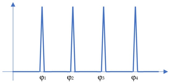
Figure 2.
Dirac comb.
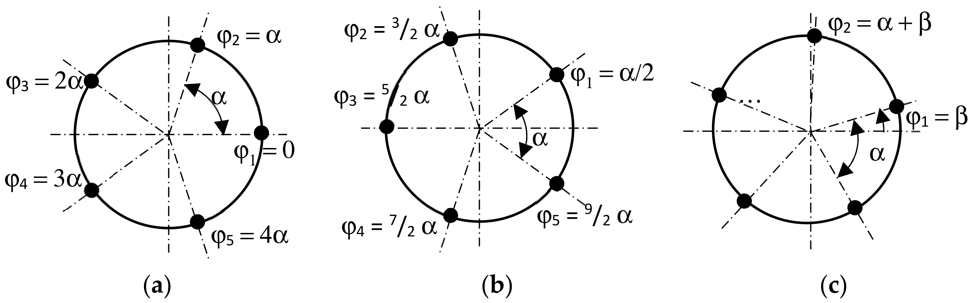
Formula (6) can be simplified, if special cases of measuring angular coordinates of piles are assumed (Figure 3).

Figure 3.
Various cases of location of piles with respect to the axes of coordinate system. (a) for φ1 = 0°, (b) for φ1 = α/2, (c) for other values of φ1.
If the angle φ1 = 0° is attributed to the pile 1 (Figure 3a), then for the load presented in Figure 2 the integrals from Formula (6) are equal to:
Thus,
It is easy to note a following feature: as m is always an integer number, then,
Therefore, if φ1 = 0, then only w0 and wm for m = in, i ∈ Z, are taken in further calculation (i.e., for m being an integer multiple of the number of piles). It must be noted that w0 is a solution for a plate subjected to a uniform load. Moreover, the more concentrated forces it is applied on a circle (i.e., the more piles support the plate), the more rarely a non-zero term occurs in the series; if there was an infinite number of piles (uniform load, continuous support), then all terms in the series would assume the zero value and only w0 would be taken for calculations.
If the angle equal to the half of the angular distance between the piles is attributed to the pile 1 (Figure 3b), then as well, but,
Due to that, if φ1 = α/2, then also only w0 and wm for m = in, i ∈ Z, are taken in further calculation but these terms will have alternately different signs (starting from the positive w0).
If, however, the angle of the first pile is different than 0 or α/2, then and qm(r) assumes other values than in (14) and (15).
The configuration of the plate examined in the paper is presented in Figure 4. The plate has j rings, wherein a ring with the number i (i = 1, …, j) is limited by the radii Ri and Ri+1 (i.e., there are j + 1 radii). The radius R1 is the radius of a post supporting the plate. Each ring has the plate stiffness and the Poisson number νi. The coefficients A0–D0 and Am–Dm in Formulas (9), (10) are being sought from:
- continuity conditions:where qm(Ri+1) are forces defined by Formulas (14), (15) and applied on the radius Ri+1, in particular equal to 0,
- boundary conditions for the clamped internal ring:
- boundary conditions for the hinged internal ring:
- boundary conditions for the external ring (free edge):
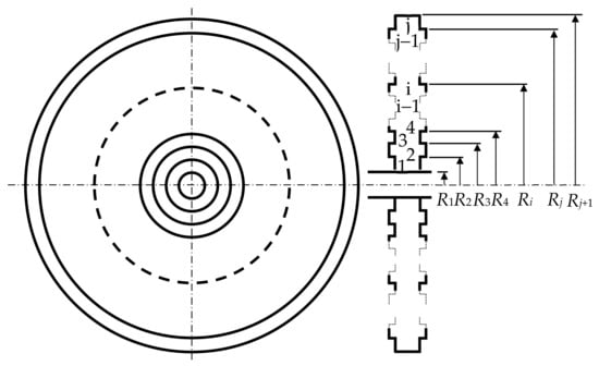
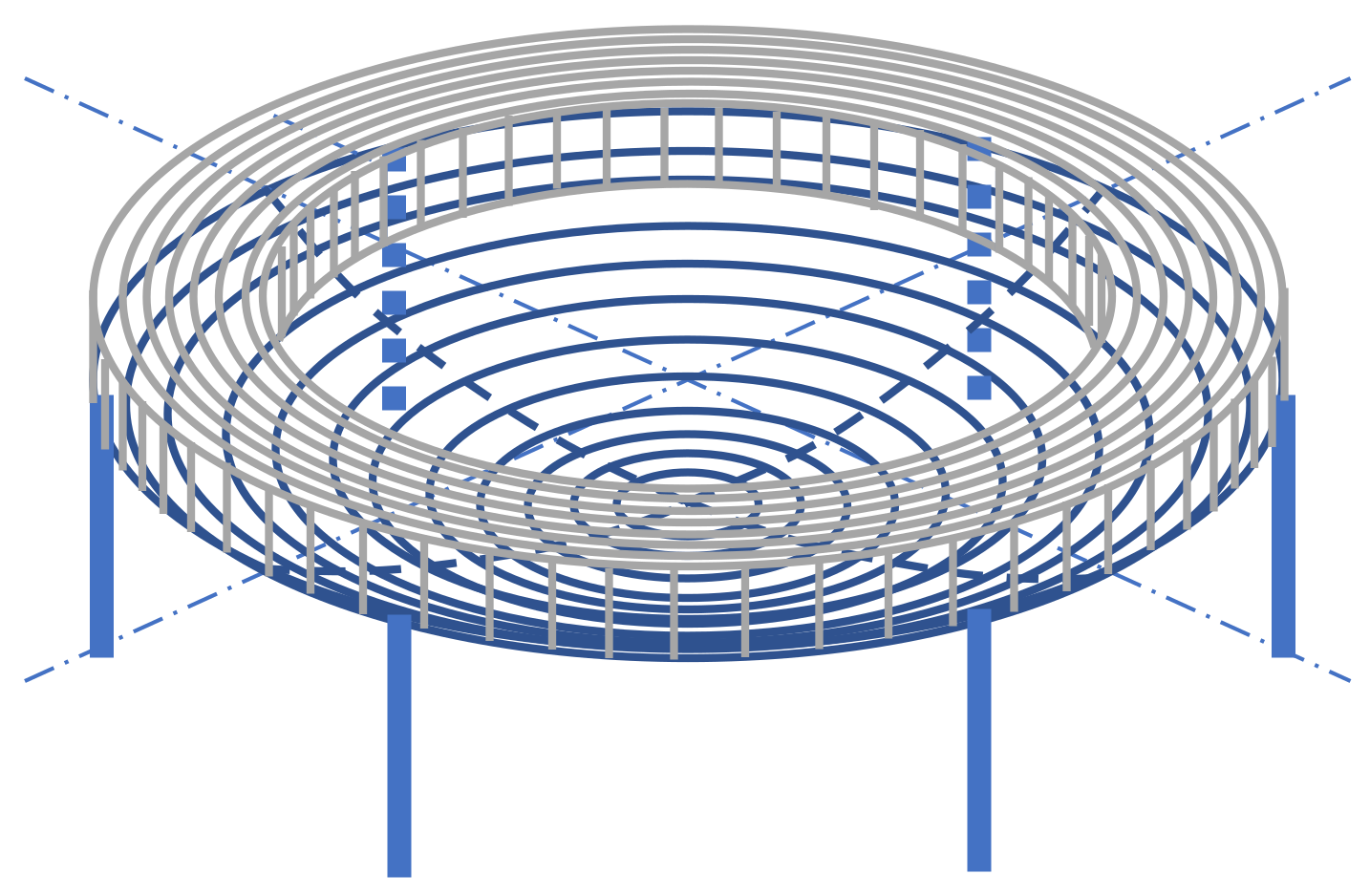
Figure 4.
General configuration of the plate analyzed in the paper.
Figure 4.
General configuration of the plate analyzed in the paper.

The individual quantities in Formulas (16)–(19) are equal to:
- slope angle:
- radial bending moment (acc. (2)):
- radial shear force (acc. (4)):
If some ring of the plate is subjected to a uniform load q, then its deflection is described by Formula (9) with a particular integral added:
In a similar way, the remaining quantities (slope angle, radial bending moment, radial shear force) require adding appropriate particular integrals:
3. Calculational Examples and Their Results
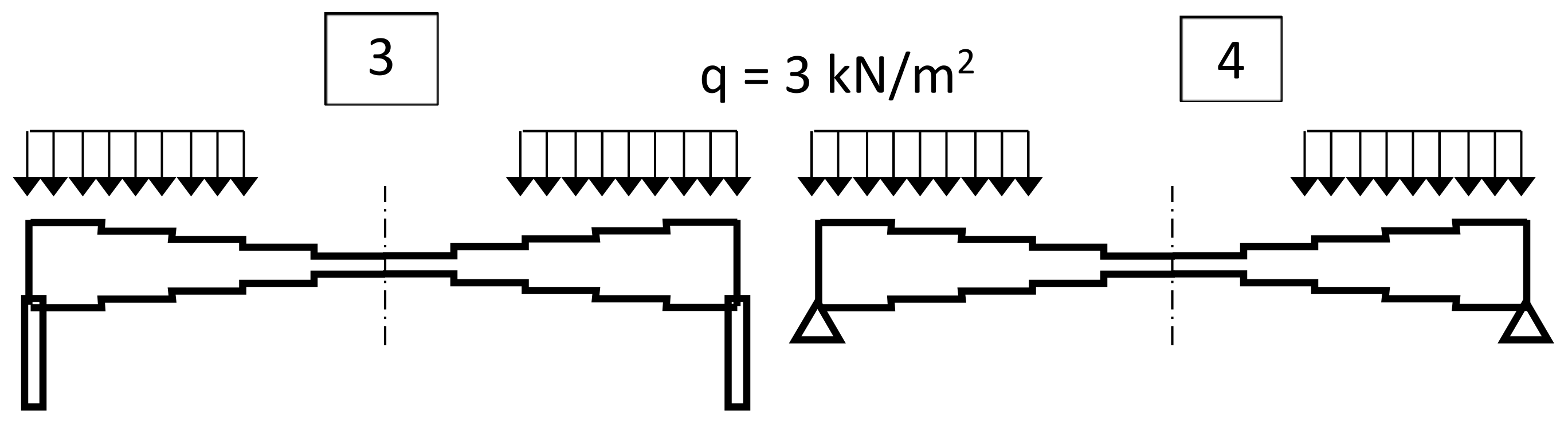
The plates presented in this paper in general have a form as in Figure 4, Figure 5, Figure 7, Figure 11 and Figure 17, i.e.,
- one can distinguish rings in the plates between which there is a discontinuous boundary,
- the plates are subjected to a surface load q on several external rings—here: q = 3 kN/m2 on three rings,
- the plates are supported on piles attributed to the circumferential circle and occasionally to an internal circle,
- there are six evenly distributed piles on each circle.
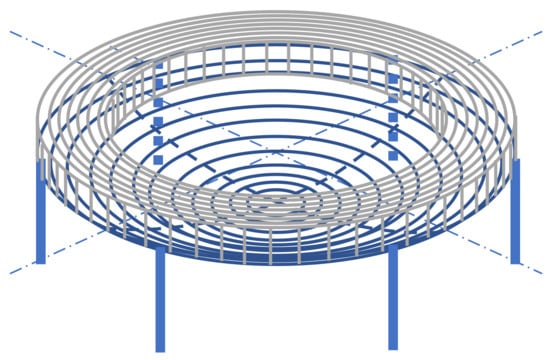
Figure 5.
General shape of the plates analyzed in the calculational examples.
Figure 5.
General shape of the plates analyzed in the calculational examples.
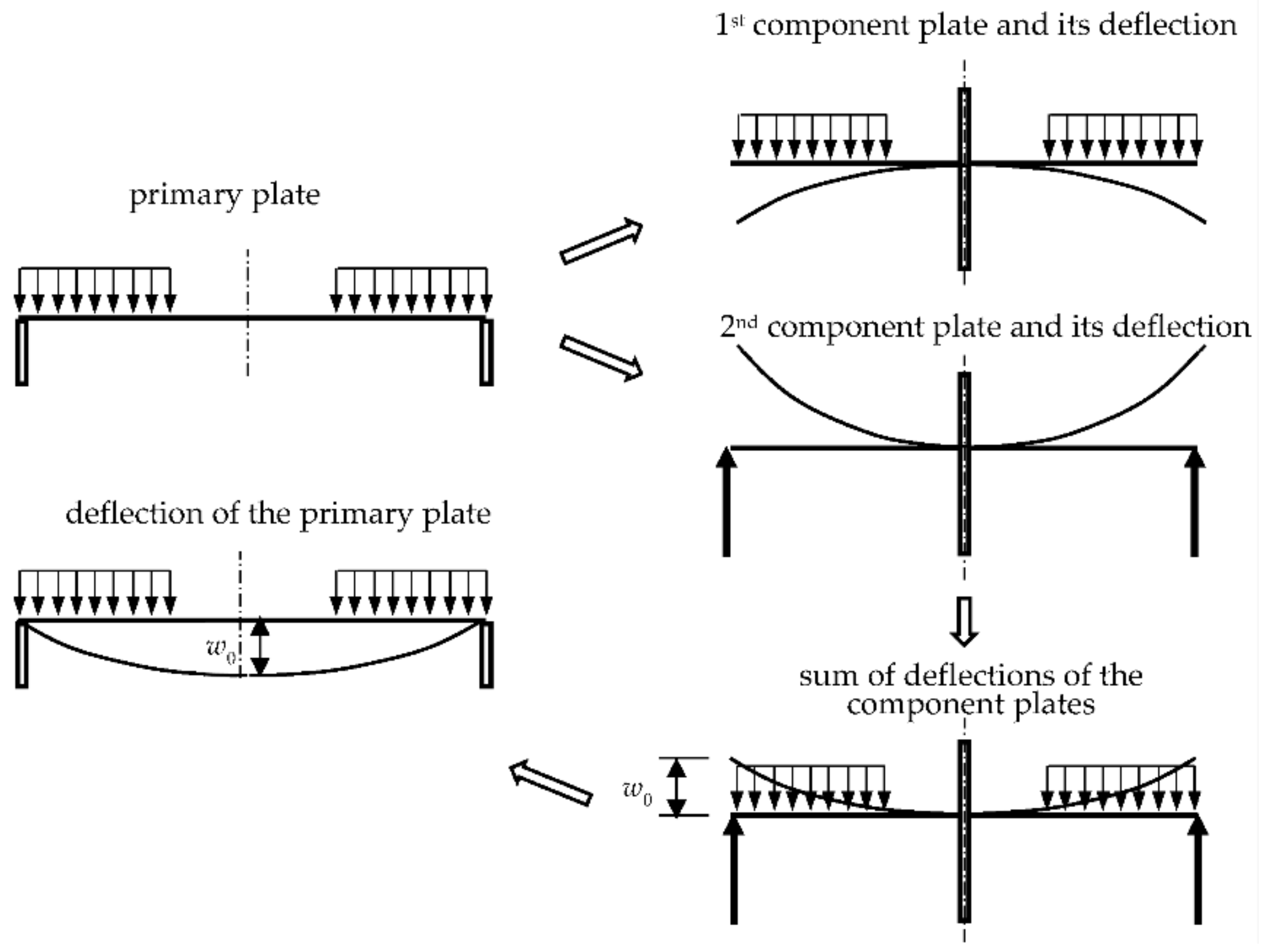
The plates in the examples have the radius 8 m and five rings separated with the radii 1.6, 3.2, 4.8 and 6.4 m. For them, it has been assumed the material with the elasticity modulus E = 36,000 MPa and the Poisson number ν = 0.25. According to the superposition rule, each plate has been divided into two: one of them is subjected to the load q and the another—with concentrated forces applied on the circumference and replacing the piles, i.e., equal to reactions in the primary plate. These two component plates are supported (clamped) on a middle post with the radius 0.2 m (arbitrarily chosen but small if compared to the radius of the smallest ring). After calculation of deflections and internal forces, the related quantities from both plates must be added to each other and the deflections additionally should be supplemented with the deflection corresponding to the radius of the circle where the forces have been applied (i.e., that circle where in fact the piles are mounted). In this operation, of course, the sign of the deflection must be considered, wherein the positive deflection in this paper is the deflection directed downward. The shape of the final deflection surface is the same as the shape of the deflected primary plate. The procedure of calculation of the deflection is presented in Figure 6.

Figure 6.
Calculation procedure for the plates being considered.
3.1. Plate with Alternately Variable Stiffness
The plate calculated in this Subsection is presented in Figure 7 and has been marked with 1. The thickness of the thinner rings has been assumed h = 0.1 m, hence their plate stiffness is equal to Nm. The stiffness of the thicker rings has been assumed as twice as the thinner ones, i.e., their thickness is 1.2 times higher. The plate has been divided into two ones: one (1a) is subjected to the load q and the another (1b)—with concentrated forces applied on the circumference and replacing the reactions in the piles, thus equal to . For the plate 1b, two sets of equations must be arranged: the first of them serves to calculate the coefficients A0–D0 and uses equations and Formulas (16a) (where Pi+1 = 0) and (17a), (19a)–(22a), whereas the second one serves to calculate the coefficients Am–Dm and uses equations and Formulas (16b) and (17b), (19b)–(22b). According to Formulas (14) and (15) and its comment, only the terms Am−Dm with subscripts m being multiple of n = 6 (number of piles) must be taken to the calculations. These sets are following:

Figure 7.
Plate for the example 3.1.
- for the coefficients A0–D0:
- for the coefficients Am–Dm:
Thus, the coefficients A0–D0 have constant values, whereas the coefficients Am–Dm depend on m. Four terms have been taken to the calculations—for m equal to 0, 6, 12 and 18. The bracketed superscripts (e.g., j in ) denote the number of a related ring.
For the plate 1a, the equations and Formulas (16a), (17a), (19a)–(22a) must be used with consideration of the particular integrals (23), (24). It results in a set:
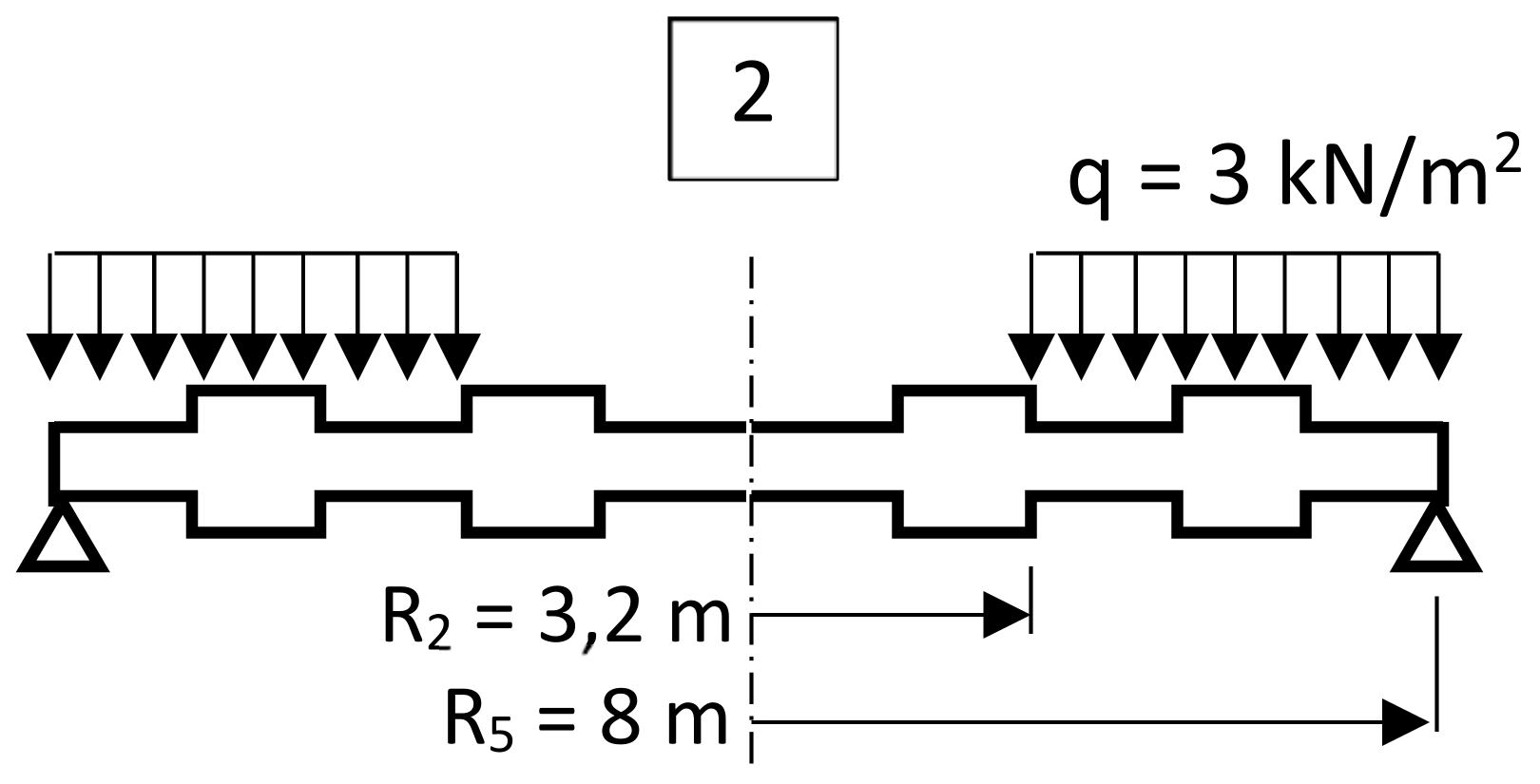
As a comparison, a plate 2 has been solved (Figure 8), where the stiffness variability and load are the same as for the plate 1 but it is simply supported on the whole circumference (a hoop instead of piles). The continuity conditions for the plate 2 are the same as for the plate 1, whereas the boundary conditions are following:

Figure 8.
Comparative plate for the example 3.1.
However, the radius in the denominators of the formulas for the slope angle and radial shear force (Formulas (20) and (22)) causes that the two first conditions (28) cannot be written for r = 0, what implies that the plate 2 must be also clamped on a post with a small radius R0, but vertically movable:
It has been assumed R0 = 0.2 m.
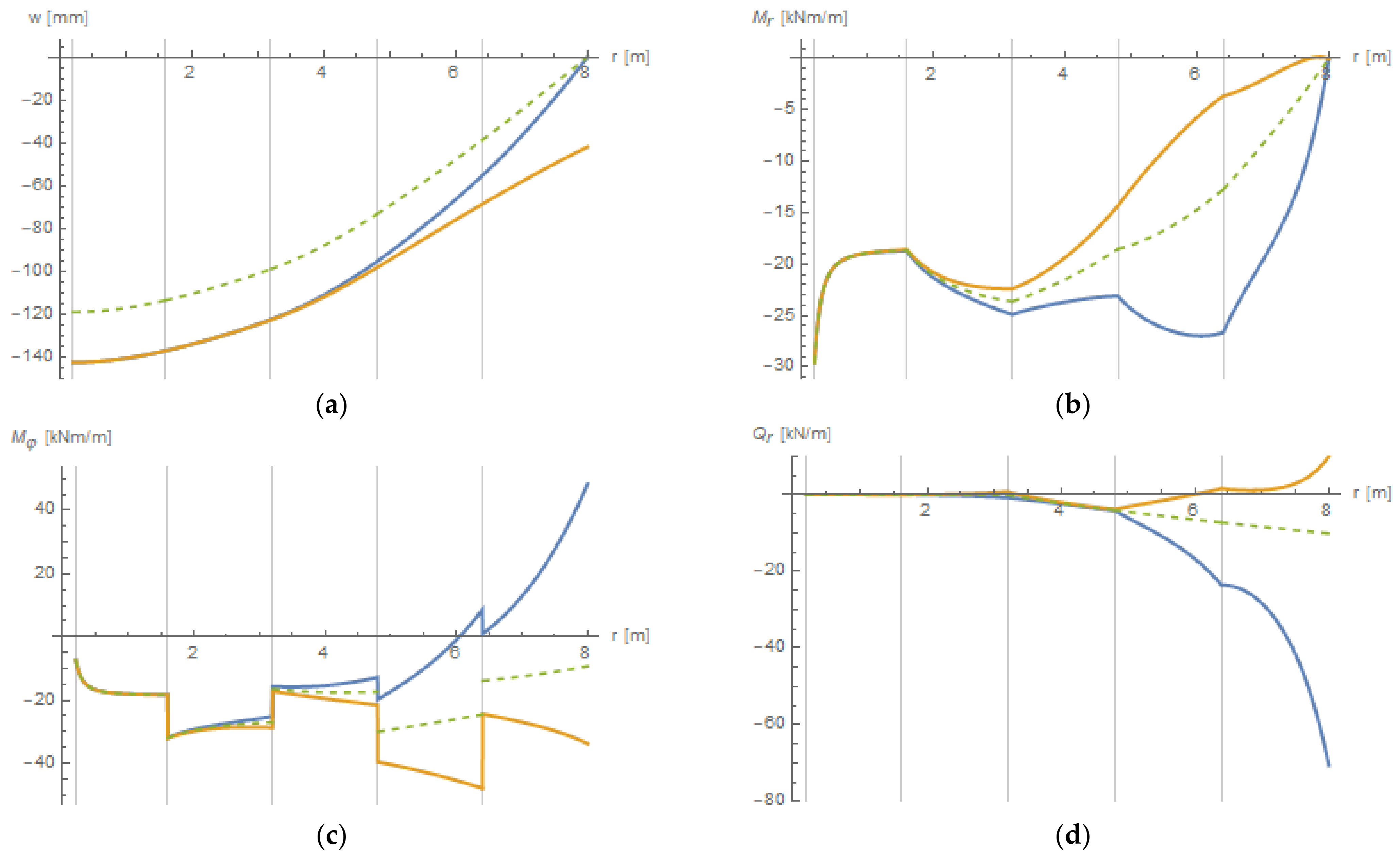
The plates 1 and 2 have been calculated in the environment MATHEMATICA®. Results (deflection w, radial moment Mr, tangential moment Mφ, radial force Qr) are presented in Figure 9 and Figure 10. Figure 9 presents relations between the given quantity and a radial coordinate in both of these plates, wherein for the plate 1—for the radii corresponding to the angle φ = 0 and φ = π/6 rad (the radius in the middle of the angular distance between the piles). Figure 10 presents the results for the plate 1 as contour maps obtained in MATHEMATICA (left) compared to results obtained in a professional FEM-based computational environment for design and calculations of building constructions—ROBOT Autodesk (right). This environment enables fast applying a geometry of a construction (as a drawing), supports and loads. The plate has been drawn as a set of coaxial, stiffly connected rings, each with the width and load according to Figure 7. Each ring is made of the same material—concrete of the B55 class (E = 36,000 MPa). The piles have been assumed as point hinge supports, i.e., disabling only the x-, y-, z-movements. Two types of meshing have initially been assumed—the Coons’ and Delaunay’s—but no substantial differences in results between them were noted, hence the Coons’ meshing was chosen as a default one in ROBOT. The element size has been assumed s = 0.5 m what results in 987 nodes.
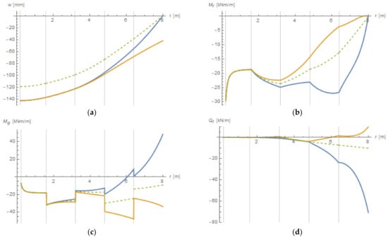
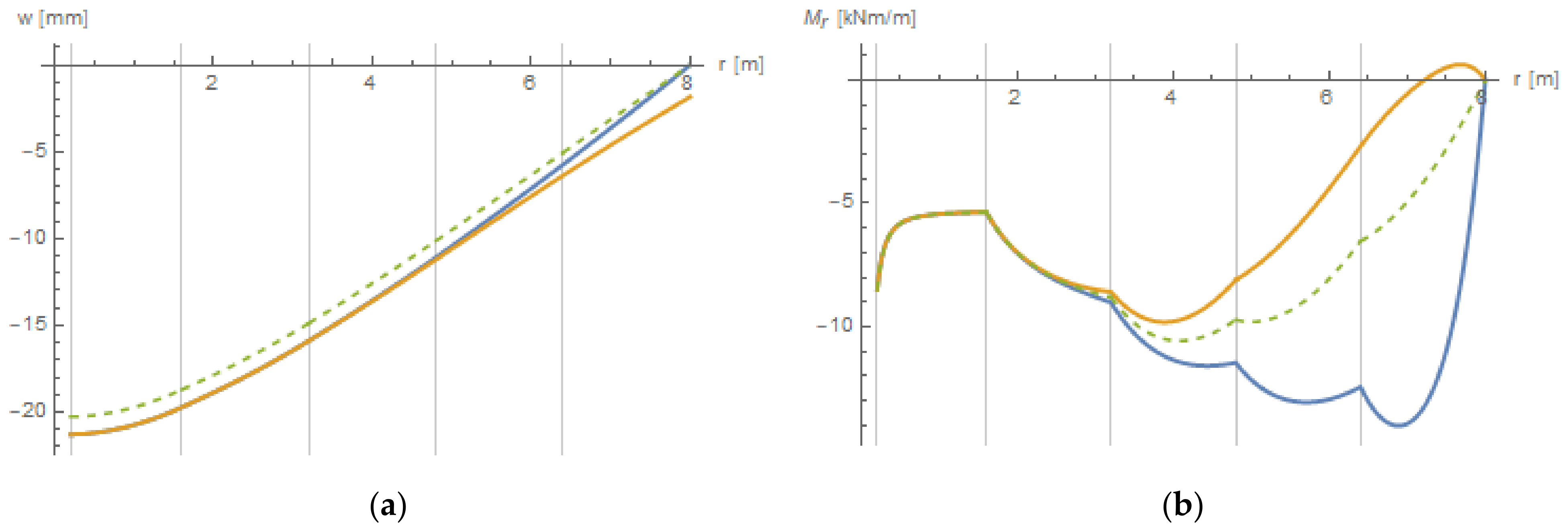
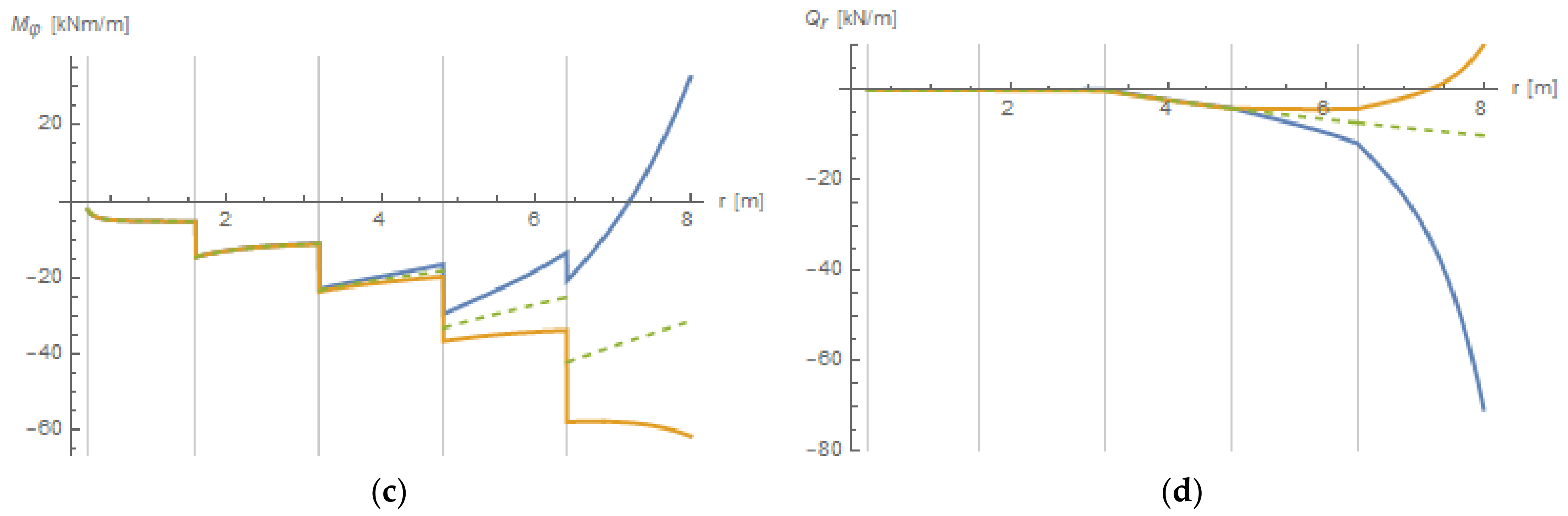
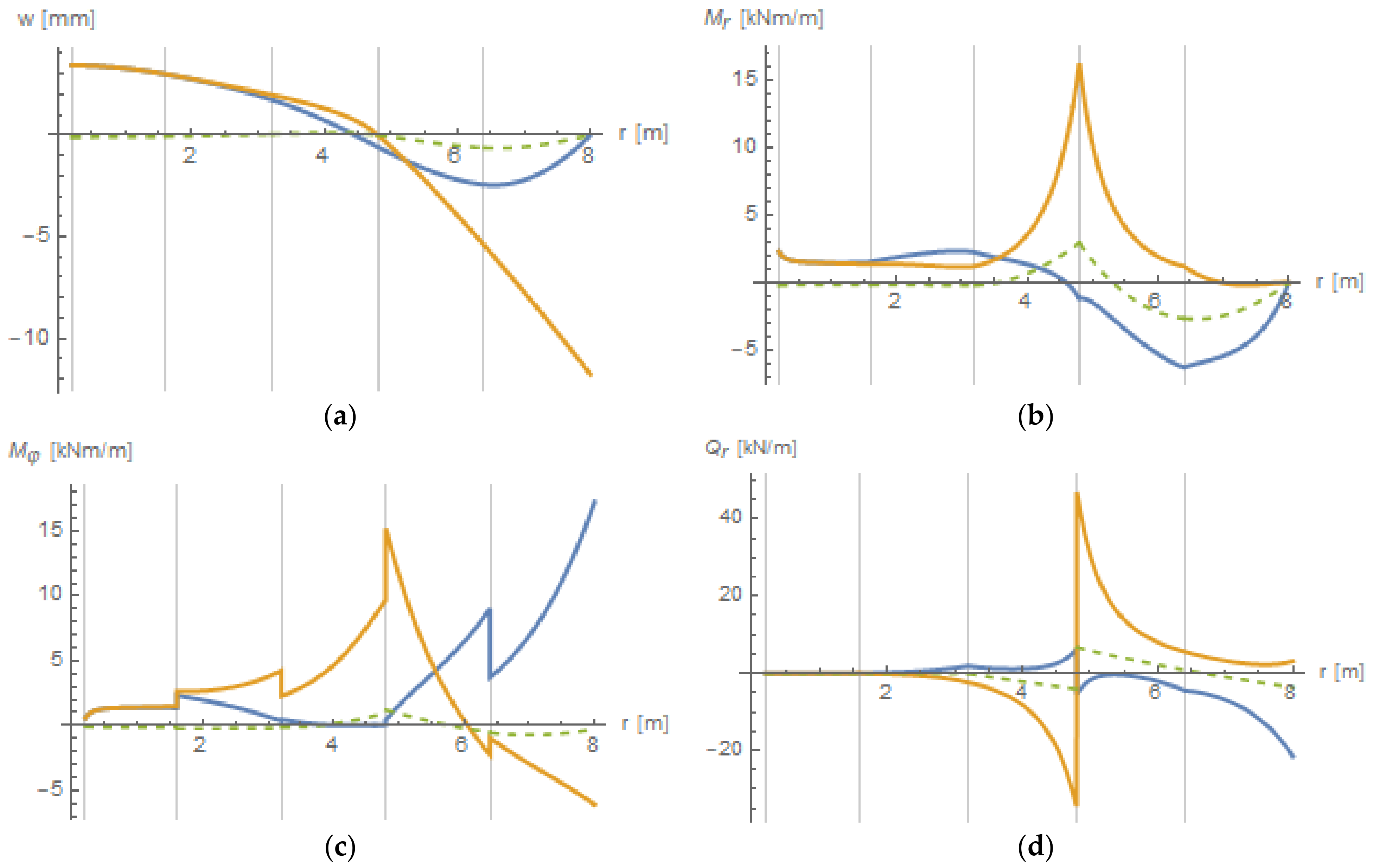
Figure 9.
Graphs for the plates 1 and 2:  plate 1, angle φ = 0,
  plate 1, angle φ = π/6,
  plate 2. (a) deflection, (b) radial moment, (c) tangential moment, (d) radial force.
plate 1, angle φ = 0, plate 1, angle φ = π/6, plate 2. (a) deflection, (b) radial moment, (c) tangential moment, (d) radial force.
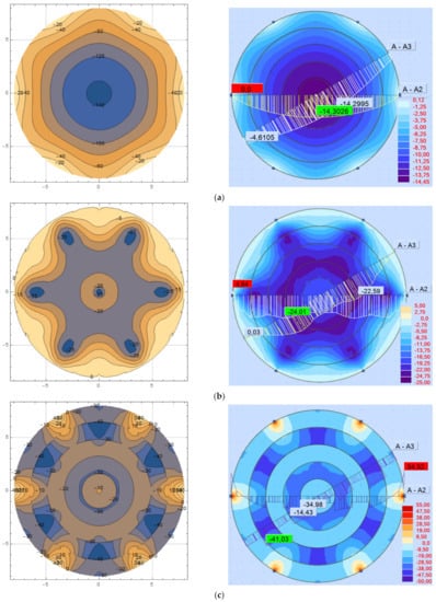
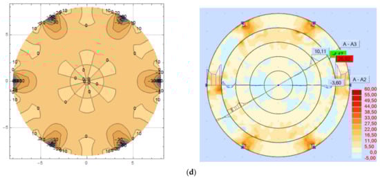
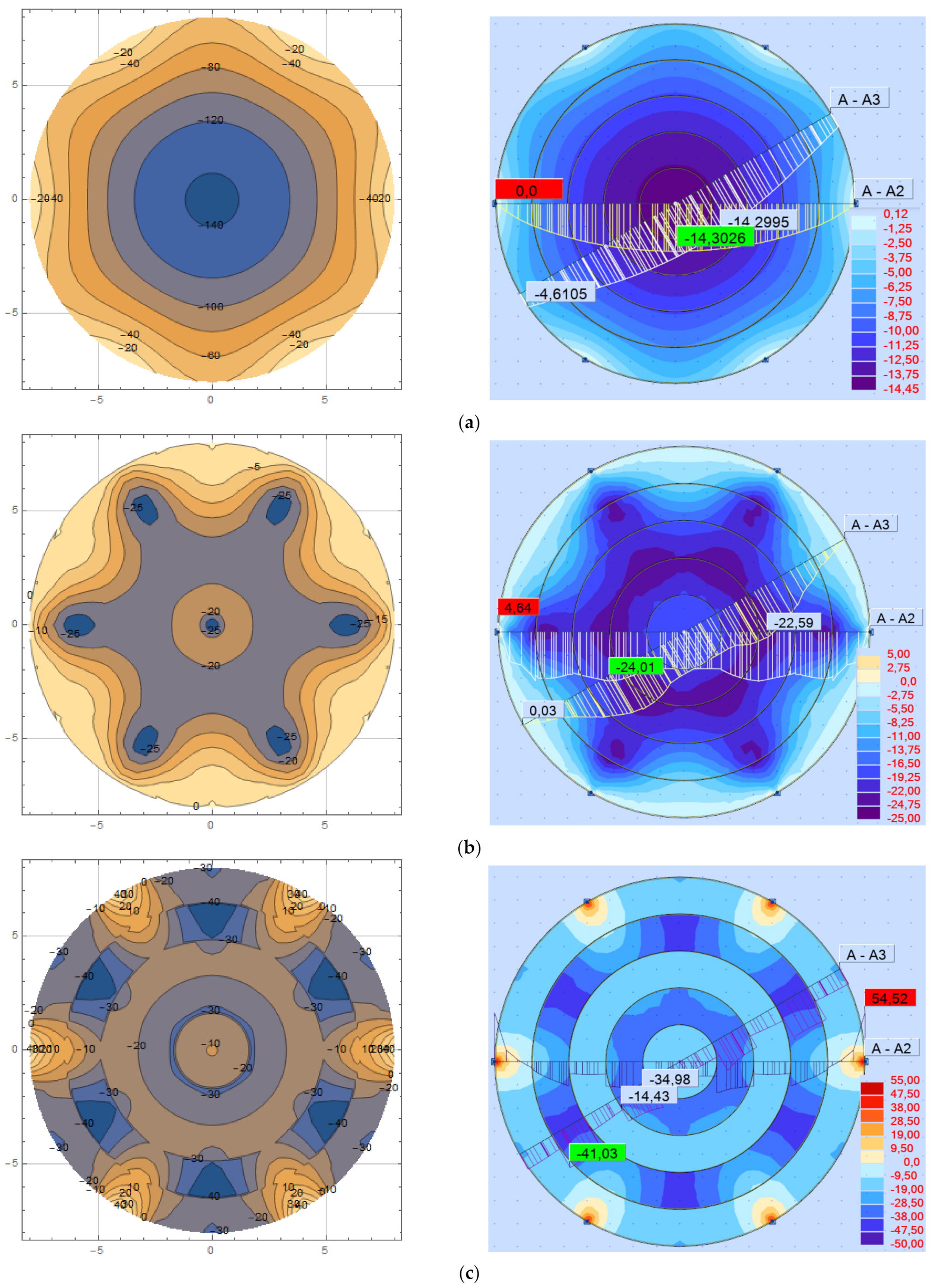
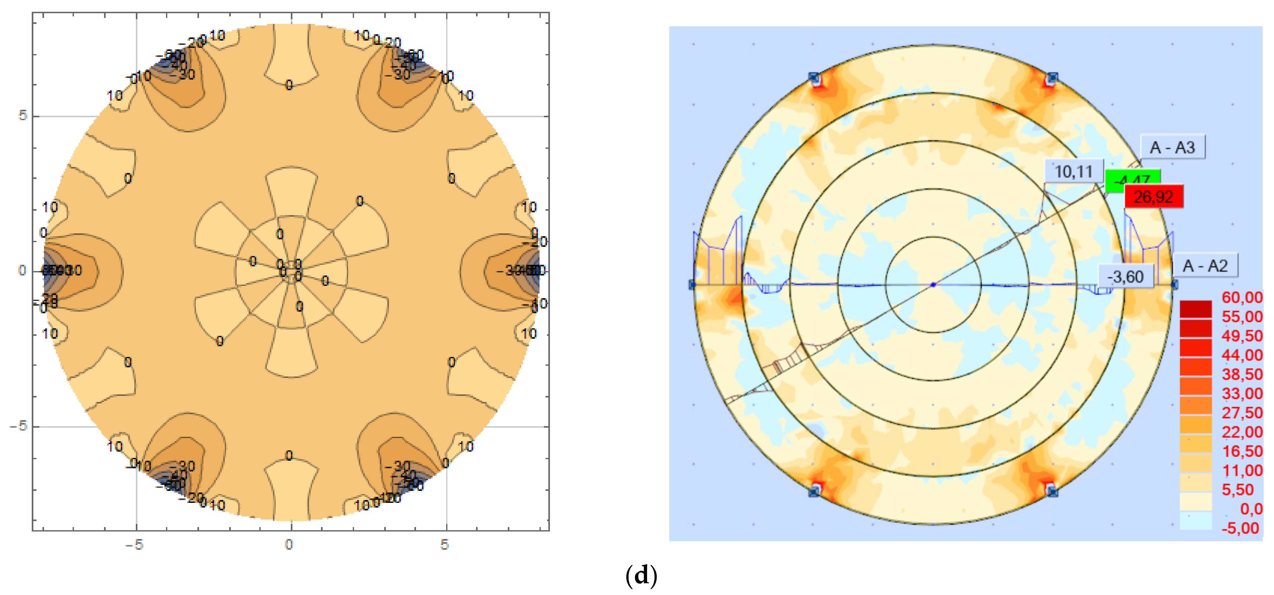
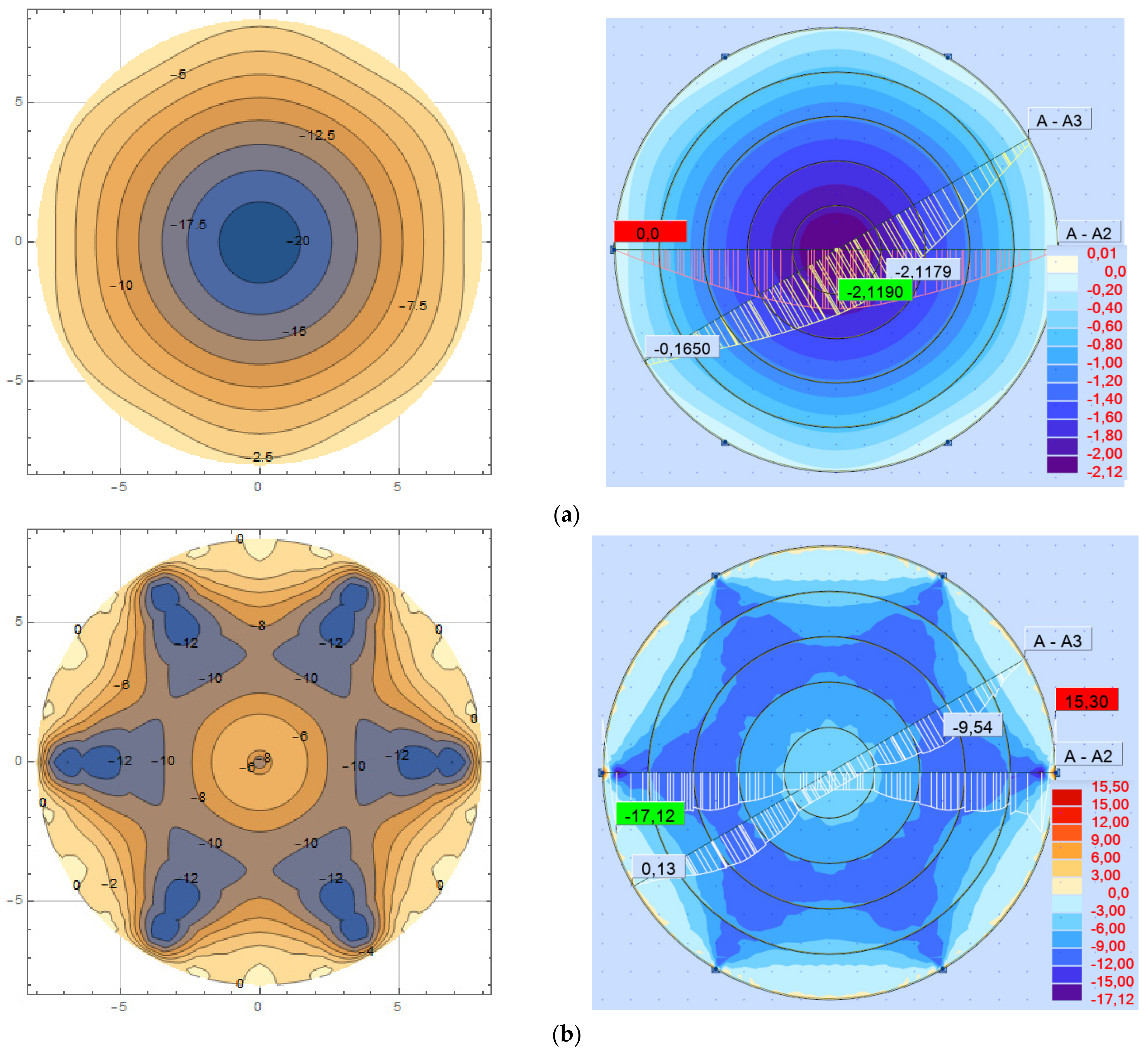
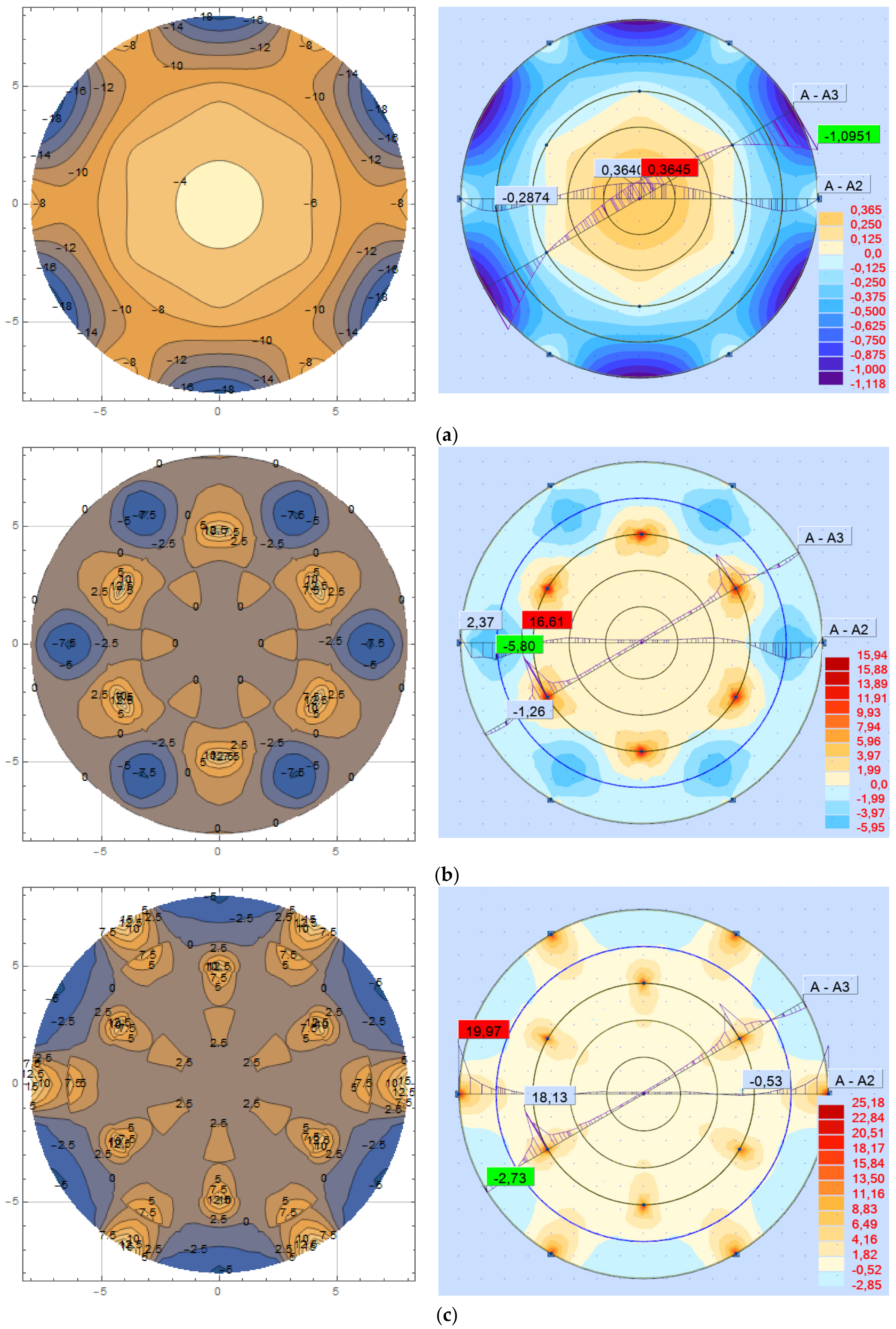
Figure 10.
Contour maps for the plate 1. In each pair, the left map has been obtained in MATHEMATICA, right—in ROBOT Autodesk. (a) deflection (left: in mm, right: in cm), (b) radial moment (in kNm/m), (c) tangential moment (in kNm/m), (d) radial force (in kN/m).
3.2. Plate with Stiffness Increasing towards the Circumference
The second example is a plate with the thickness growing stepwise from the center towards the edge. It has been denoted as 3 (Figure 11). For the plate 3, the rings have the thickness 0.1, 0.15, 0.2, 0.25 and 0.3 m. As a comparison, it has been also calculated a plate 4, having the same geometry and load but supported on a hoop instead of piles. Figure 12 presents relations for the plates 3 and 4 analogical to those in Figure 9. Figure 13 presents the results for the plate 3 as contour maps in analogical way as those in Figure 10.
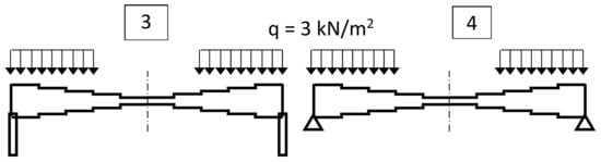
Figure 11.
Plates for the example 3.2.
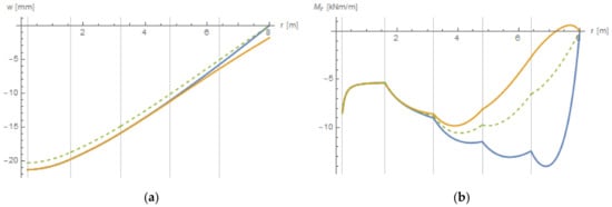
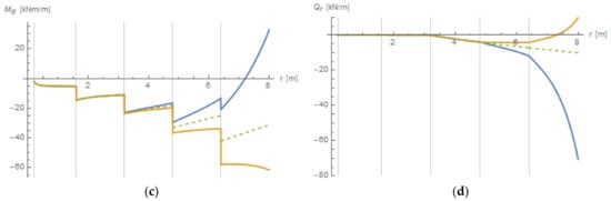
Figure 12.
Graphs for the plates 3 and 4: plate 3, angle φ = 0, plate 3, angle φ = π/6, plate 4. (a) deflection, (b) radial moment, (c) tangential moment, (d) radial force.
plate 3, angle φ = 0, plate 3, angle φ = π/6, plate 4. (a) deflection, (b) radial moment, (c) tangential moment, (d) radial force.

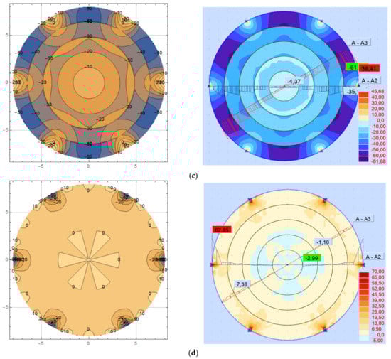
Figure 13.
Contour maps for the plate 3. In each pair, the left map has been obtained in MATHEMATICA, right—n ROBOT Autodesk. (a) deflection (left: in mm, right: in cm), (b) radial moment (in kNm/m), (c) tangential moment (in kNm/m), (d) radial force (in kN/m).
3.3. Comparative Examples—Plates with Continuously Variable Stiffnesses
As a comparison, plates analogical to the above ones but with the continuously variable stiffness (thickness) have been calculated—supported both on piles and on a hoop (Figure 14).

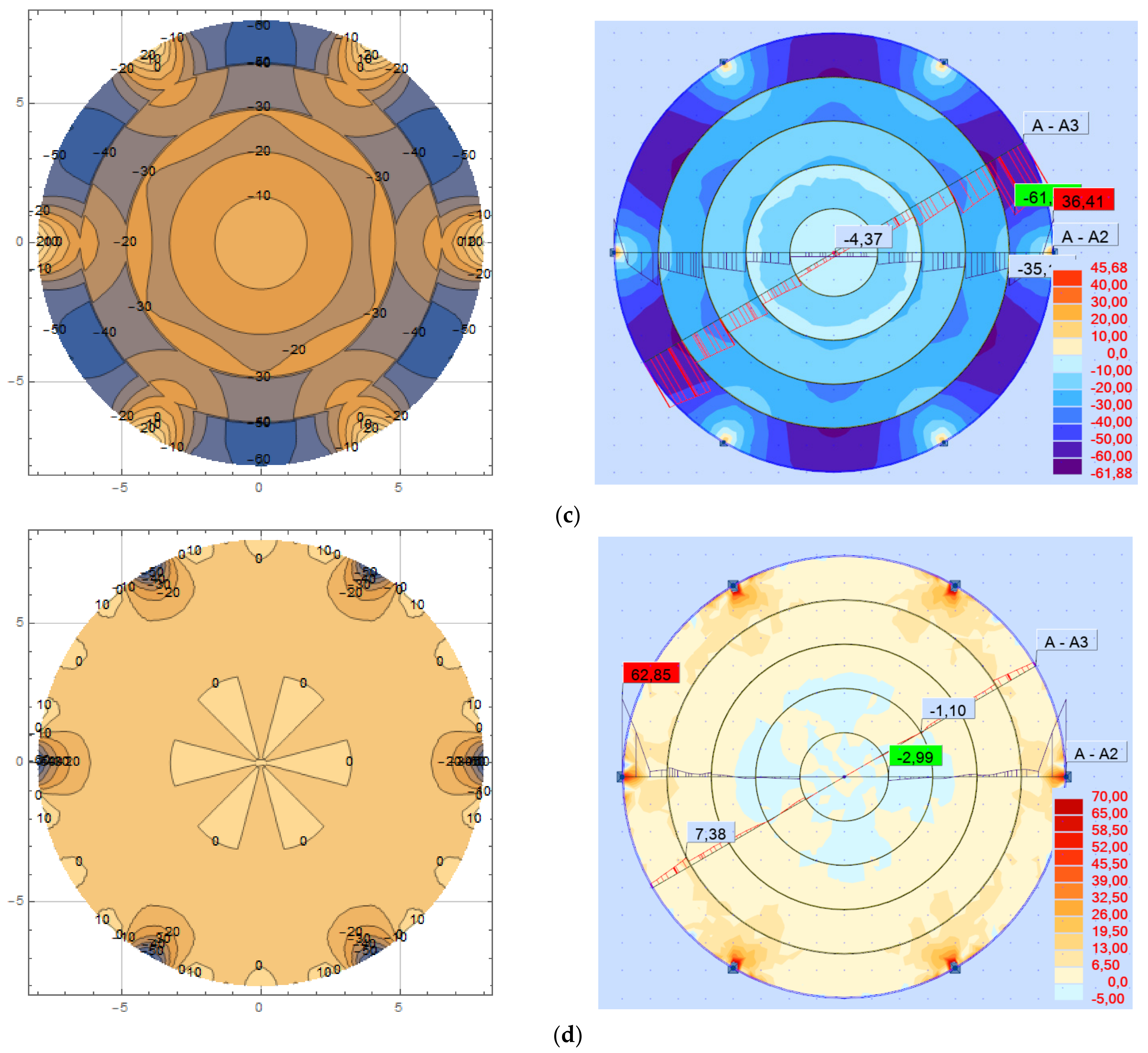
Figure 14.
Plates for the example 3.3.
The plates denoted as 5 and 6 are equivalents of the plates 1 and 2, respectively; if compared to the plates 1 and 2, as the most similar relation describing the stiffness variability, a sinusoidal relation has been recognized in the form:
The plates denoted as 7 and 8 are equivalents of the plates 3 and 4; their stiffness varies according to the formula:
where, for the assumed dimensions of the plates, a = 0.025, b = 0.1 m (for r = 0: h = 0.1 m, for r = 8 m: h = 0.3 m).
A circular plate having a stiffness variable along the radius but constant in the tangent direction, and loaded with forces variable in the tangential direction, will be subjected to a deflection varying both in the radial and in the tangent direction. The relations for such plate are following [3]:
- equation of deflection:
- radial shear force:
The formula for the radial bending moment (2) remains without changes.
It is impossible to solve analytically the Equation (32) for the assumed stiffness function and boundary conditions. For the plates 6 and 8, there is no dependence in the tangential direction (on the angular coordinate φ) what implies that the related derivatives become equal to 0 and such equation can be solved with the command NDSolve in the MATHEMATICA. However, the equation in the full form (plates 5 and 7) can be solved only numerically—e.g., with use of the final difference method (use of the command NDSolve causes that the deflections are unreal and the radial moments and forces do not satisfy boundary conditions, the more the smaller is the radius R0). The FDM mesh size has been assumed 0.1 m. The quantities obtained for the plates 5–8 are presented in Figure 15 and Figure 16.
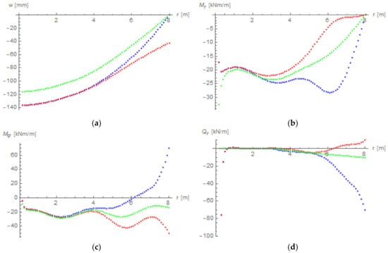
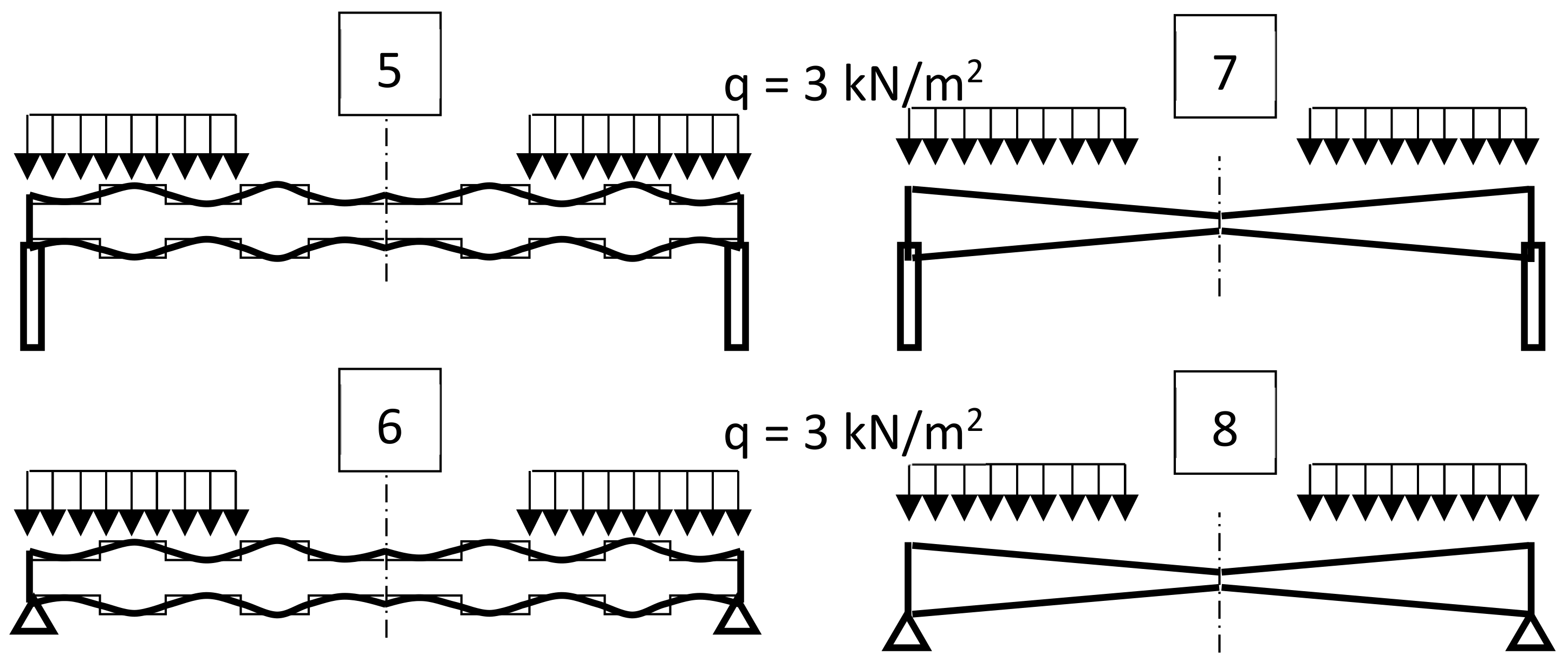
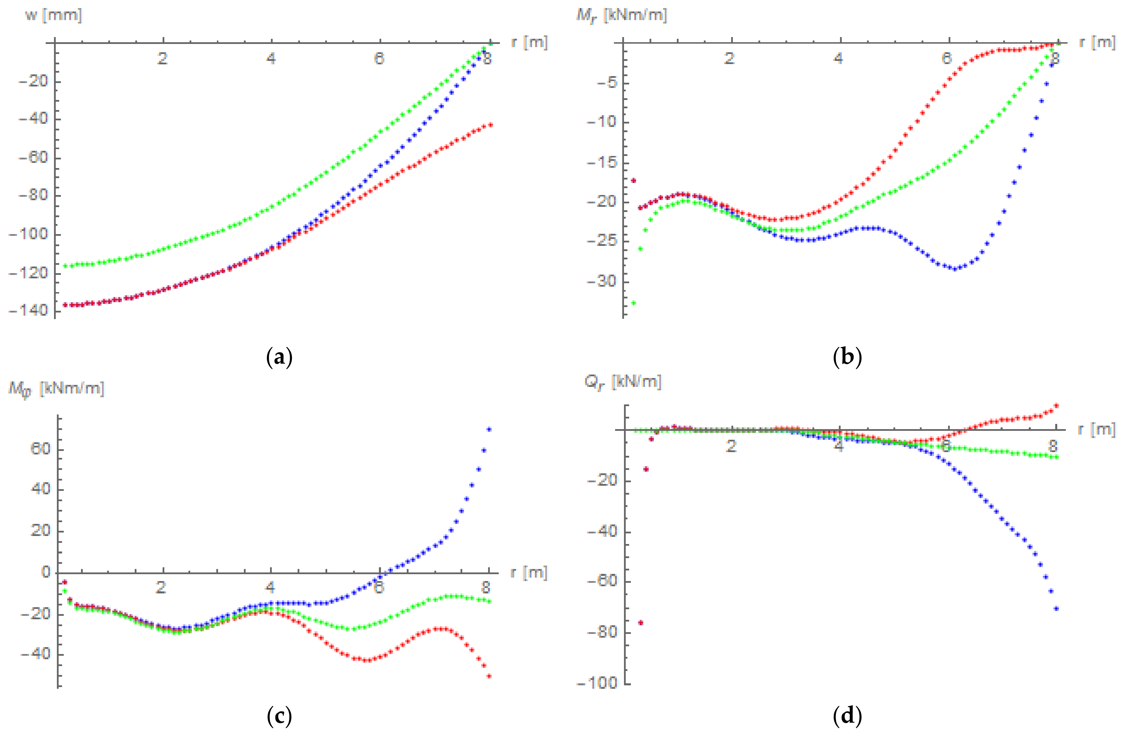
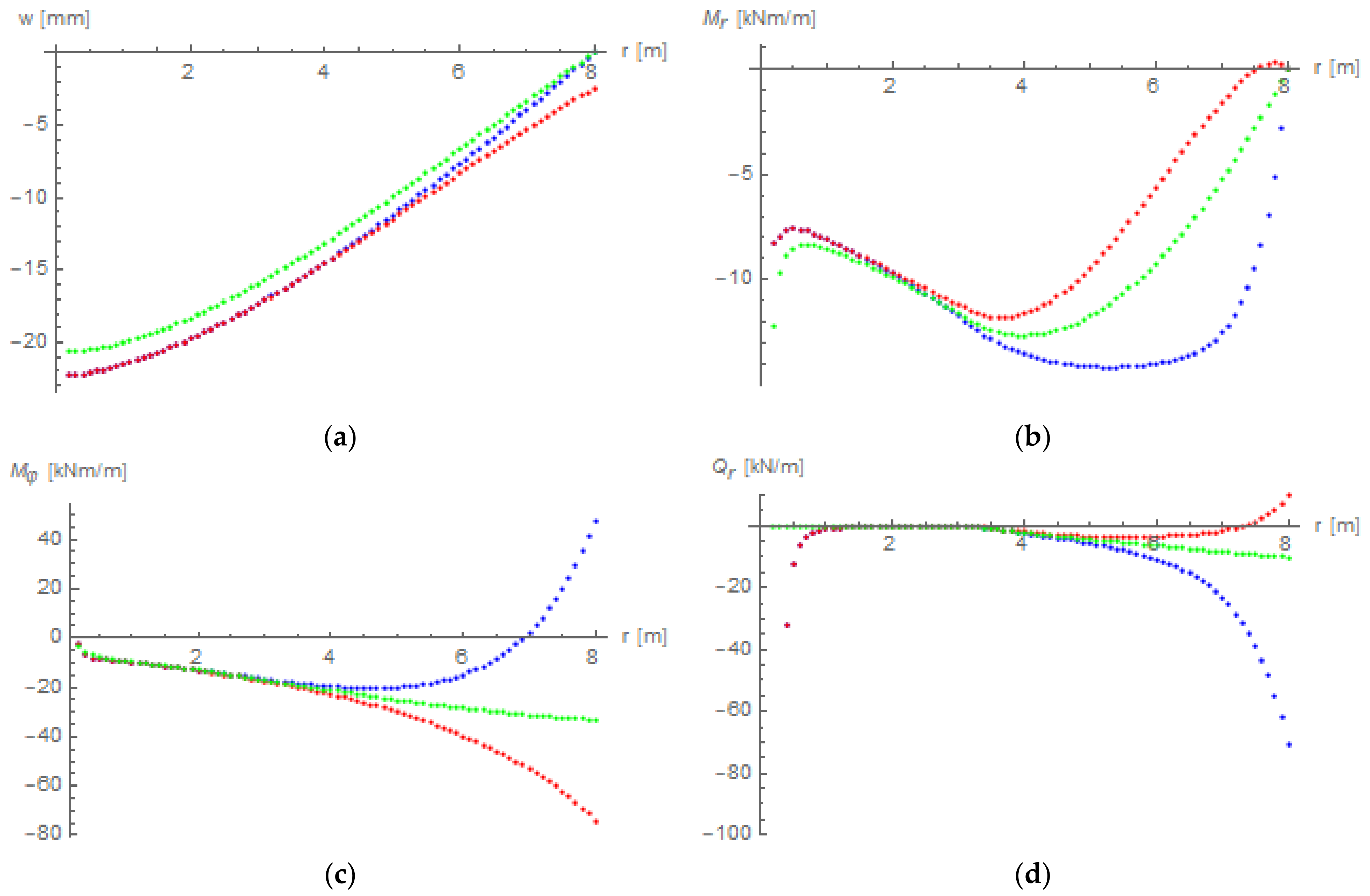
Figure 15.
Graphs for the plates 5 and 6: ●●● plate 5, angle φ = 0, ●●● plate 5, angle φ = π/6, ●●● plate 6. (a) deflection, (b) radial moment, (c) tangential moment, (d) radial force.
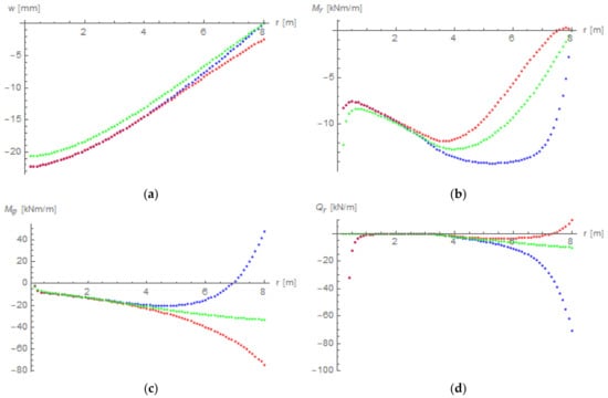
Figure 16.
Graphs for the plates 7 and 8: ●●● plate 7, angle φ = 0, ●●● plate 7, angle φ = π/6, ●●● plate 8. (a) deflection, (b) radial moment, (c) tangential moment, (d) radial force.
3.4. Plate Supported on Two Rows of Piles
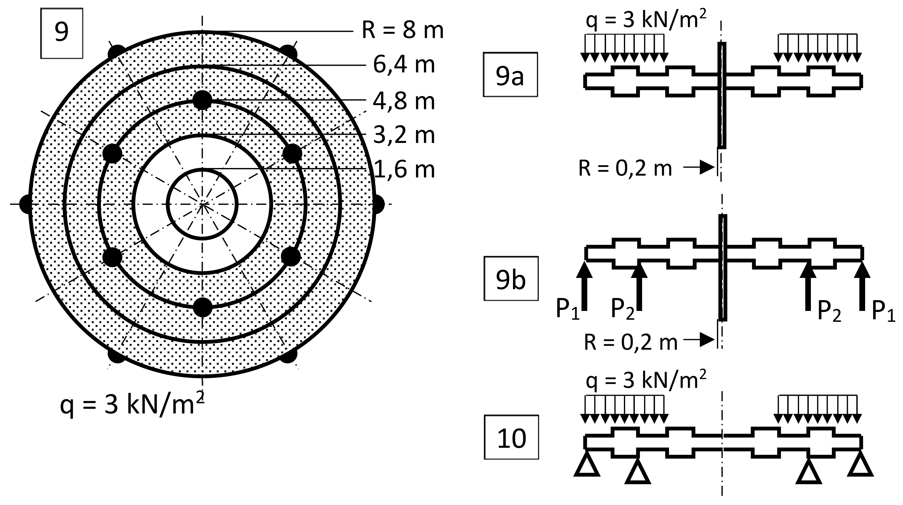
The plate presented in Figure 17 and marked as 9 has been also calculated. It has two rows of piles: an internal row with the radius 4.8 m and an external row with the radius 8 m, each of them with 6 piles, wherein the internal ones are shifted in tangential direction with the angle π/6 rad relative to the external piles. The surface load acts also between the radii 3.2 and 8 m. The stiffness varies in the same way as for the plates 1 and 2. As a comparison, it has been solved an analogical plate but supported on a hoop.

Figure 17.
Plates for the example 3.4.
In the continuity conditions (16), for the radius R3, corresponding to the internal piles, it is,
The basic difficulty consists here in establishing reactions in piles, hence the forces P for the plate 9b. The forces P1 and P2 are different, though the same on a given pile row (they would be different if the internal and external rows had different number of piles). The solution to the plate 10 is helpful in this situation. It is a plate similar to the plate 2, however in the Formula (16), the conditions , must be replaced by , . The obtained reactions on the hoops are: 10.748 kN/m on the internal hoop, 3.631 kN/m on the external one (cf. Figure 18a). If each of these (continuous) forces is distributed on 6 piles, then, for the internal and external row of piles in the plate 9b, one obtains, respectively:
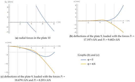
Figure 18.
Procedure of establishing the forces P1 and P2 for the plate 9b. Graph (a) enables to calculate reactions in the plate 10. These reactions give forces for a trial calculation of Graph (b)—the deflections are unreal, no conformity between the deflections in points with the coordinates (r, φ) = (8, 0) and (r, φ) = (4.8, π/6). Graph (c) shows this conformity, thus the forces P are proper.
Then, it must be checked if such forces ensure that after adding the deflections of the plates 9a and 9b the deflection of the primary plate 9 in a point corresponding to any external pile (R = 8 m), e.g., for the angle 0, is equal to the deflection in a point corresponding to any internal pile (R = 4.8 m), e.g., for the angle π/6 rad. If this is not the case (Figure 18b), then, using the trials-and-errors method, it must be found such forces P1 and P2 whose sum is always equal to 26.88π kN and which ensure the abovementioned equality of deflections. For the plate 9, it has been established in this way: P1 = 18.679π kN and P2 = 8.201π kN. Finally, the deflection graph must be moved by the value of the deflection corresponding to the radius of position of any pile—in this case, the graph had to be lifted by 3.424 mm (Figure 18c). The final results are presented in Figure 19 and Figure 20.
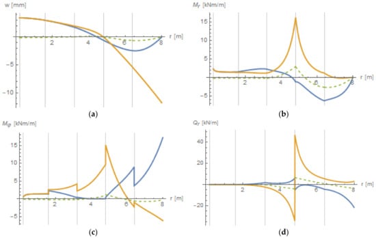
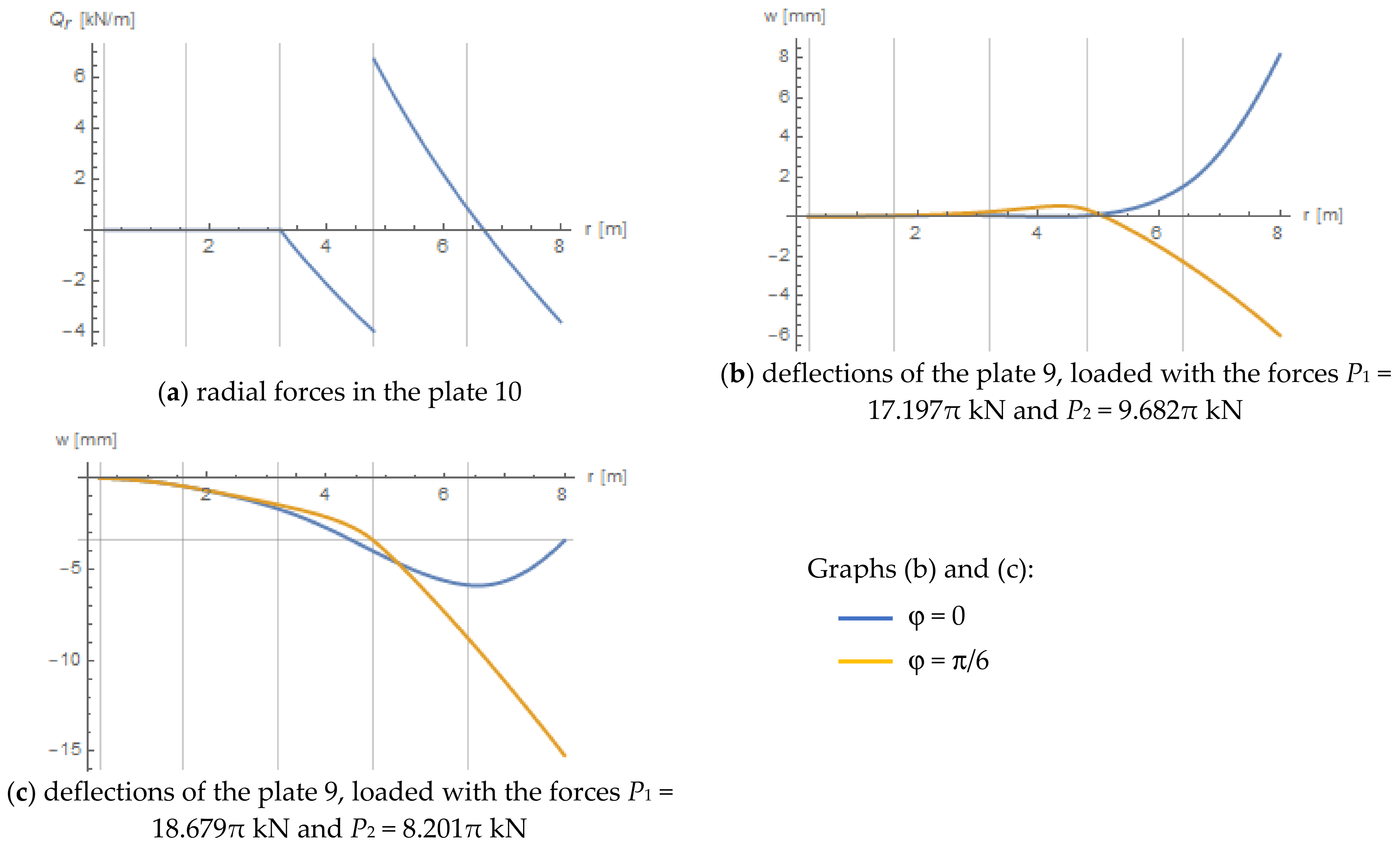
Figure 19.
Graphs for the plates 9 and 10: plate 9, angle φ = 0, plate 9, angle φ = π/6, plate 10. (a) deflection, (b) radial moment, (c) tangential moment, (d) radial force.
plate 9, angle φ = 0, plate 9, angle φ = π/6, plate 10. (a) deflection, (b) radial moment, (c) tangential moment, (d) radial force.
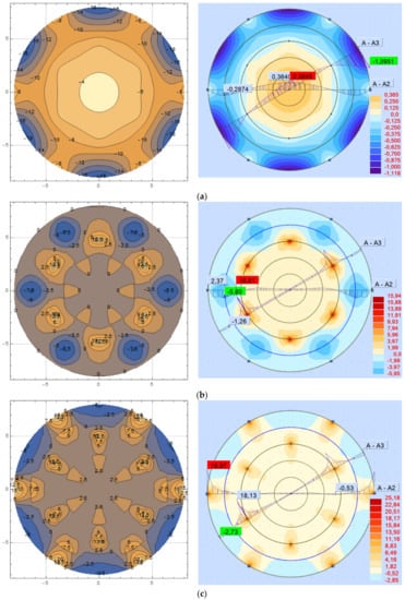

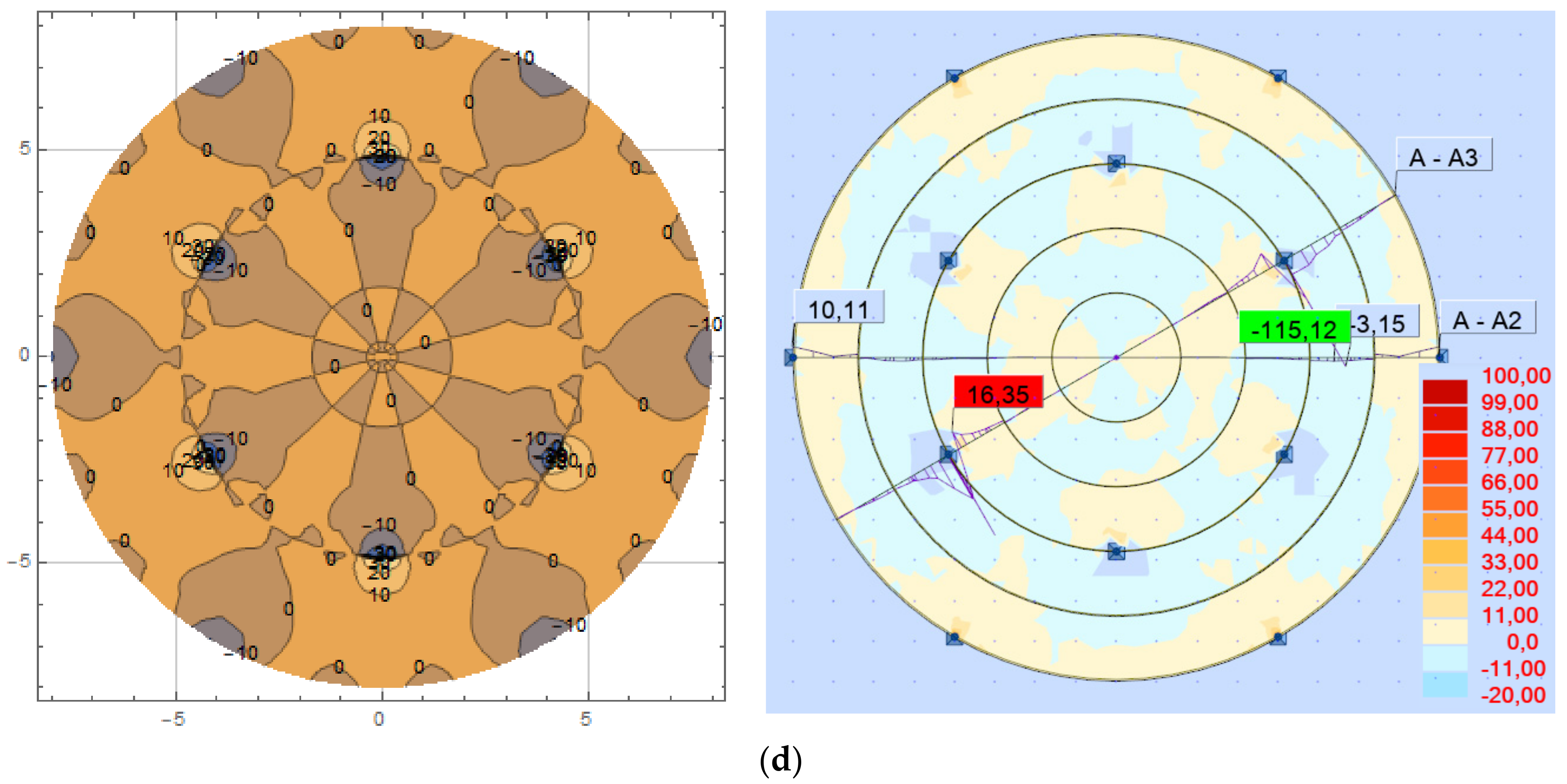
Figure 20.
Contour maps for the plate 9. In each pair, the left map has been obtained in MATHEMATICA, right—in ROBOT Autodesk. (a) deflection (left: in mm, right: in cm), (b) radial moment (in kNm/m), (c) tangential moment (in kNm/m), (d) radial force (in kN/m).
4. Discussion of Results and Convergence Analysis
As seen in the graphs and maps, the maximum deflection of the plate 2 is lower than of the plate 1, similar relation is between the plates 4 and 3, 6 and 5, 8 and 7—the plates 1, 3, 5, 7 have more freedom in movement on the circumference. For the plates 9 and 10, this effect is glaring in the face. The radial and tangential bending moments for the plates 2, 4, 6, 8 are approximately a mean of the moments for the plates 1, 3, 5, 7, respectively; this effect is very weak for the plates 9 and 10. A sudden fall visible in the graphs of the radial moments in the vicinity of the plate center and an analogical rise in the graphs of the tangential moments (both would be visible in the 3D polar graphs as “funnels” directed upward or downward) are due to the fact that during the calculations the narrow post had to be placed there (cf. Figure 7) and the more the radius of this post is, the higher the radial and the lower the tangential bending moments are. Of course, there should not be any fall or rise—this is only a calculational side effect. The differences between the plates supported on piles and on a hoop in the graphs increase along with the growth in the distance from the plate center.
The most positive tangential moments for the plates supported on piles are just over the piles—the plate is bent most in the tangential direction exactly over there. The most negative tangential moment is in a midpoint between the piles. The shape of the graph of the tangential moment reflects the dependence of the stiffness on the radial coordinate.
The graphs of radial shear forces require a broader discussion. It results from the graphs for the plates 1, 3, 5, 7 that the force over the pile is equal to 70.56 kN/m, whereas the reaction should be 26.88π = 88.45 kN. It is due to the fact that the piles are modelled as a point, hence the concentrated force is applied in point. As it was mentioned above, only four terms have been taken to the calculations—this is enough for the accuracy of calculations of the deflection and moments, taking more terms does not improve the results significantly. However, it is different for the forces. If a force is applied in a point, hence on a zero area (length), then the value in the graph should go to infinity—it is indeed the case if the number of terms is being increased what results from the formula for expansion of the Dirac delta/comb function in a trigonometric series. In aim to obtain a real value of the reaction in the graph, it should be assumed some dimensions of the pile, and the load—not as a concentrated force but a load distributed on some area what complicates the calculation, not contributing significantly to its results (it should be assumed an additional ring, having width equal to the pile diameter, and another load function, e.g., series of rectangular impulses, instead of the Dirac delta/comb, but it would not affect the graphs of deflection and moments). The value of 70.56 kN/m, visible in the graph, results from the right sides of the last equations of the sets (25) and (26): for m = 0 it is kN/m, for m = 6, 12, 18 it is kN/m, hence for all these m it yields 70.56 kN/m. Thus, the graphs of the shear force are only indicative: they show that the radial shear force in the center of the plates 1 and 2 is equal to 0, the force on the circumference of the plate 2 and between the piles on the plate 1 is equal to kN/m, the shape of the whole graph is consistent with the engineer’s intuition and the superposition gives proper results. The graphs of the shear force must be treated with caution especially in the vicinity of piles.
In an analogical way, for the plate 9 it can be read from the graph of the shear forces (Figure 19d) that the reaction in the internal piles (the difference between the values from both sides of the coordinate r = 4.8 m for the orange line) is 75.07 kN/m and the reaction in the external piles (the value for the coordinate r = 8 m for the blue line) is 25.42 kN/m. In a similar way as for the plates 1, 3, 5, 7, these values are obtained as follows: for m = 0 and the internal piles (R = R4 = 4.8 m) it is kN/m, for the external piles (R = R6 = 8 m) it is 3.63 kN/m; for m = 6, 12, 18 and the internal piles it is kN/m for the external piles it is 7.26 kN/m. Hence for all these m it gives 75.07 kN/m for the internal piles and 25.41 kN/m for the external ones. The real values of reactions are 18.679π = 58.68 kN and 8.201π = 25.76 kN.
Regarding the results of FEM (ROBOT Autodesk), they must be acknowledged as less credible, though they are close to these from MATHEMATICA. It is evident that the radial bending moment has non-zero values on the circumference, hence it does not fulfill the boundary condition. The shear forces have discontinuities on the borders between the rings, hence they do not fulfill the continuity conditions, moreover the values of these forces over the piles depend on the size of the finite element and cannot be referred as reactions. The reactions are not visible in the maps because they are presented in another window in ROBOT. The reactions over the piles for the plate 1 amounted between 83.62 and 84.86 kN, hence almost equal to 26.88π, for the plate 3 it was between 83.66 and 84.84 kN. For the plate 9 it was within the range 55.85–56.11 kN for the internal piles and 28.17–28.60 kN for the external ones, thus the differences in relation to the forces obtained in MATHEMATICA are ca. ±10%.
Regarding the plates 5–8, generally, it has been stated a high concordance of the relations obtained for the plates with continuously and stepwise varying stiffness. The deflection of these plates is a bit smaller than for the corresponding plates 1–4, i.e., a plate with a stiffness varying continuously according to the assumed relations (30) and (31) is a bit stiffer than the related plate with stepwise varying stiffness (in the presented cases—ca. 2%). The conformity of the relations decreases as the order of derivatives in the formulas increases and the radial coordinate decreases. Each differentiation accentuates inaccuracies in calculations, hence the lowest conformity is for the radial shear forces in the vicinity of the radius R0 (even a sudden fall as a calculational side effect can be observed there what was not the case for the other plates).
For the plate 9, in general, it can be noted that the conformity between the results from MATHEMATICA and ROBOT Autodesk is a bit lower than for the other plates.
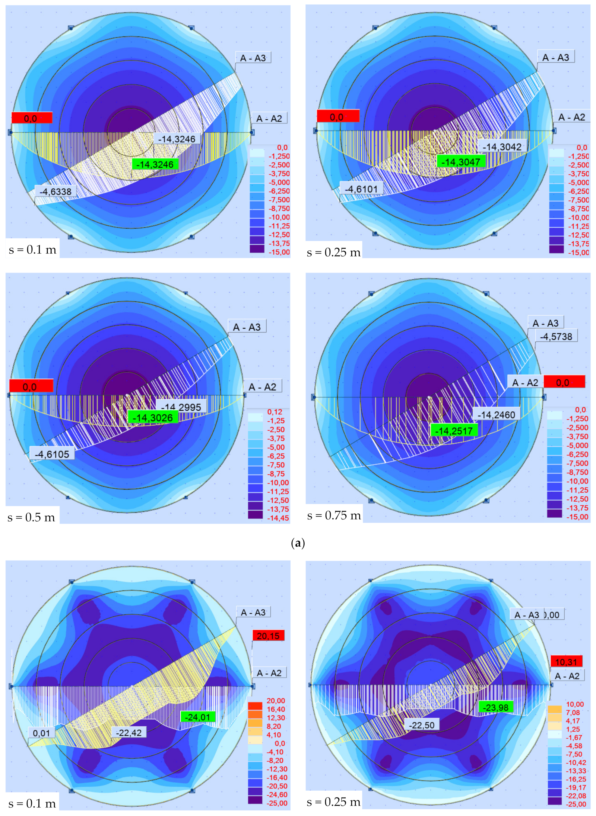
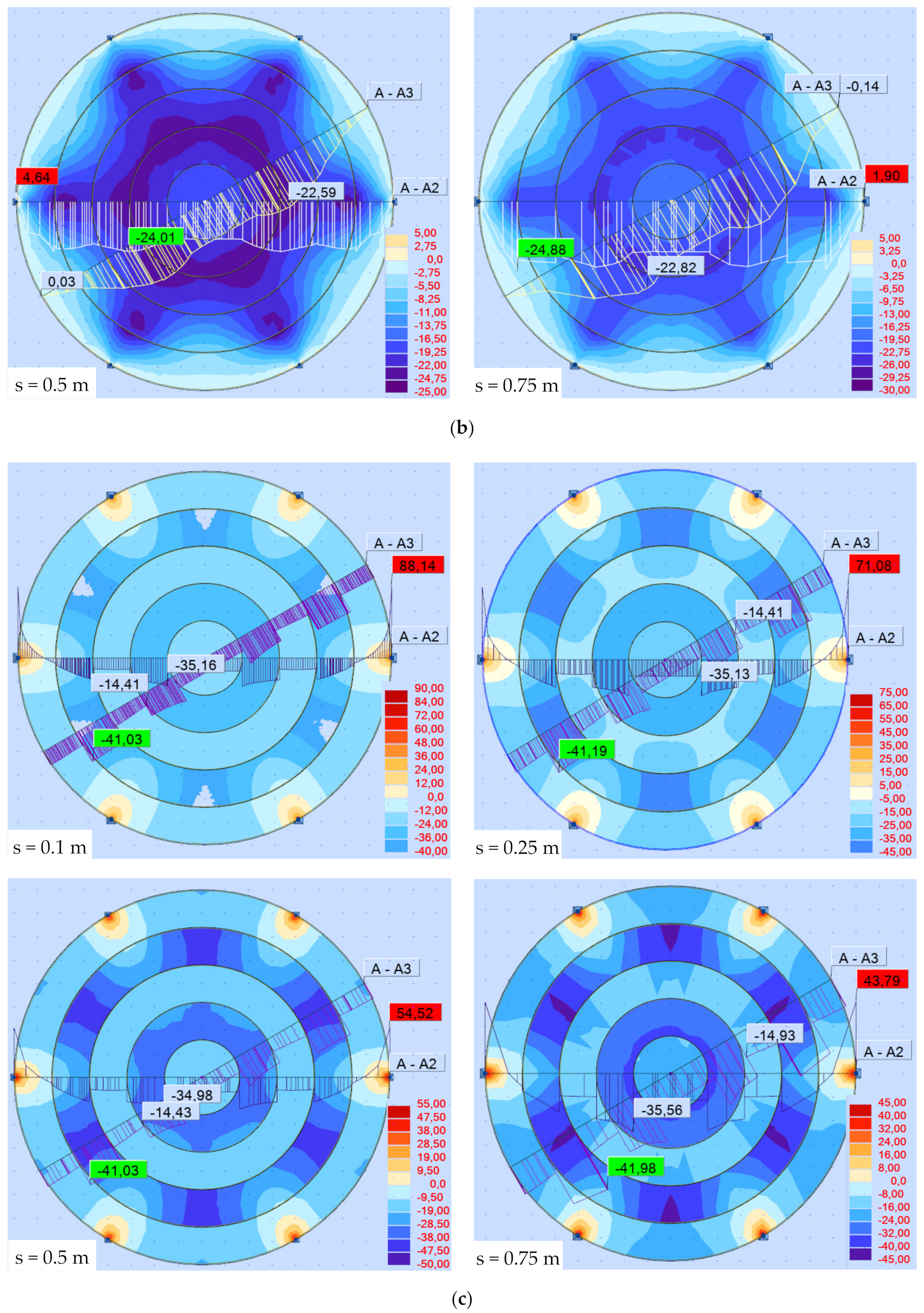
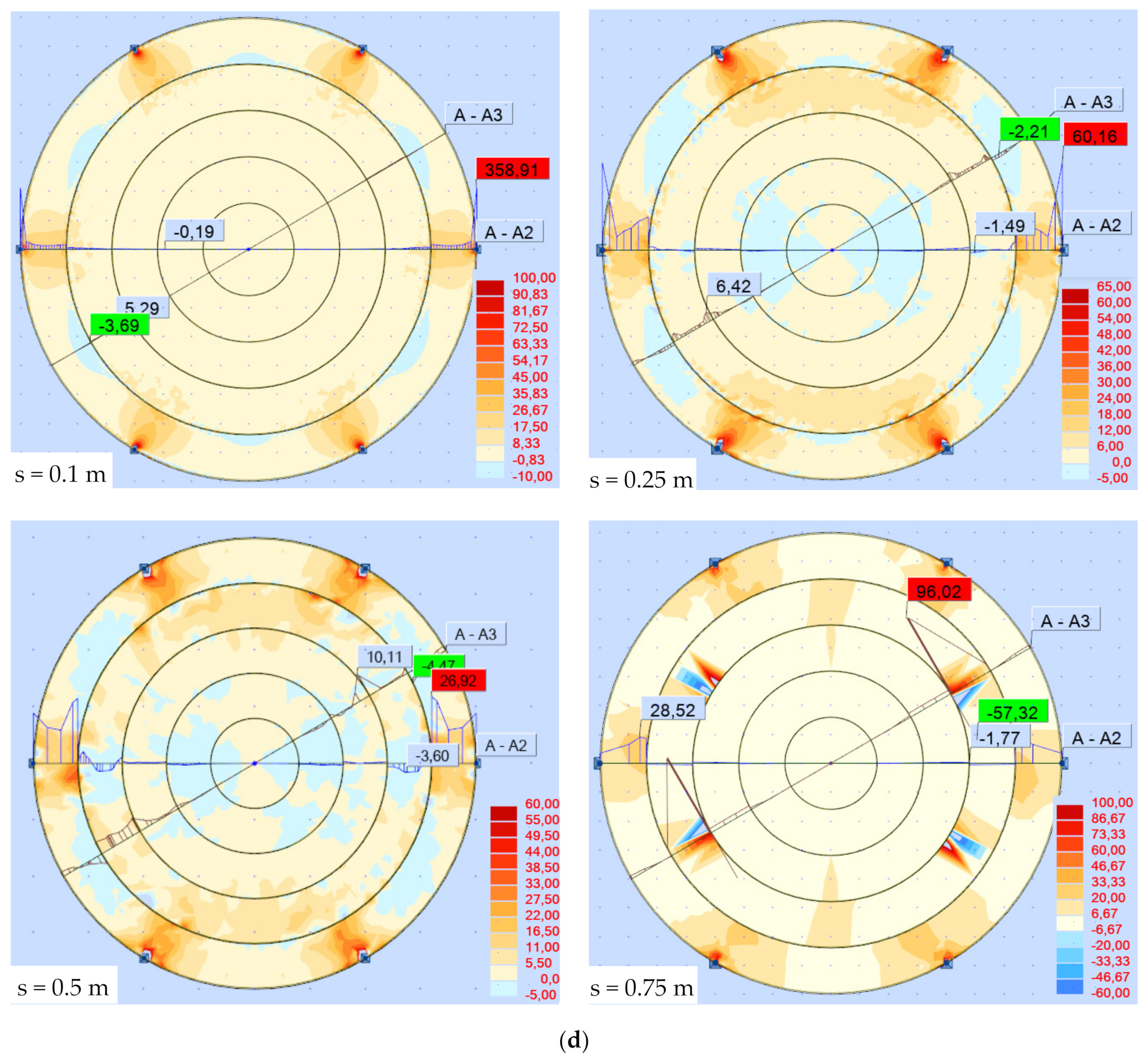
For the results from the ROBOT Autodesk, a short convergence analysis has been also performed. It consisted in checking, how the mesh size s affects the results. The analysis was performed for the plate 1 and 9. As mentioned in Section 3.1, the basic mesh size was equal to 0.5 m and all results in the contour maps of the right sides have been obtained for such size. Apart of this size, the following sizes have been assumed in the analysis: s = 0.1 m (18,714 nodes), s = 0.25 m (3525 nodes) and s = 0.75 m (454 nodes). Figure 21 shows the maps for the plate 1.
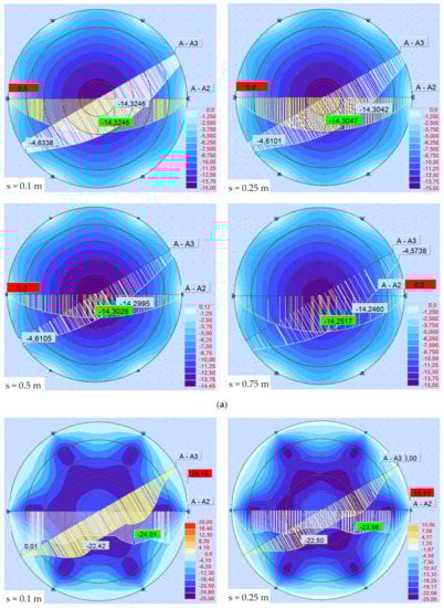
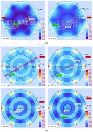
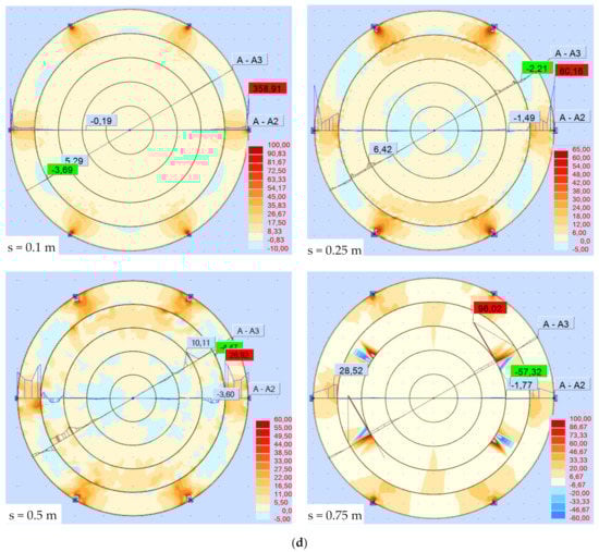
Figure 21.
ROBOT Autodesk contour maps for the plate 1 for various mesh sizes. (a) deflection [cm], (b) radial moment [kNm/m], (c) tangential moment [kNm/m], (d) radial forces [kN/m].
The purpose of these maps is to present similarities and trends in the changes of the quantities being presented. The trends and similarities are best visible in the case of the deflection, radial moment and tangential moment. The shear forces—according to the prior conclusions—are the least credible: the extreme points change their position depending on the mesh size, the values are excessively high; if the size decreases, then the values at the edge of the plate and the differences between the values at the boundaries between the rings increase.
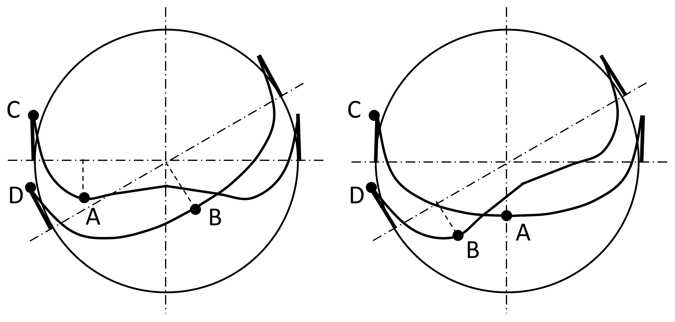
Table 1 presents the values of ordinates of characteristic points of the graphs of the deflection, radial moment and tangential moment for the plates 1 and 9. The shear forces have not been considered due to the abovementioned reasons. These characteristic points, showed in Figure 22, are: the maximum values of the quantity for the angle φ = 0° (A) and φ = 30° (B) (for each angle, it can be either one point in the plate center or two points at the same radii but opposite with respect to the plate center—as in Figure 22) as well as the edge values for the angle φ = 0° (C) and φ = 30° (D) (for the moments in the plate 9, the points B correspond to the internal supports).

Table 1.
(a) Values of the deflection, radial moment and tangential moment for various mesh sizes—plate 1. (b) Values of the deflection, radial moment and tangential moment for various mesh sizes—plate 9.
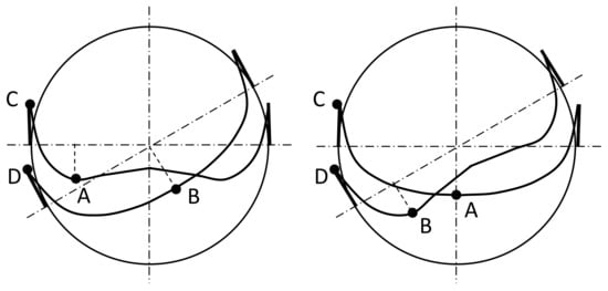
Figure 22.
Characteristic example points for the graph values in Table 1.
As seen, the worst results are for the “coarse” mesh (s = 0.75 m), what seems expectable, whereas the results for the remaining mesh sizes are close to each other and similar to those from MATHEMATICA (although, some small deviations can be visible for the finest size—s = 0.1 m). Therefore, taking calculation costs into consideration, it is enough to assume the mesh size 0.5 m (besides, it was assumed as default by ROBOT for the task being presented).
The moment values at the supports seem to be a problem, however—they increase far over the theoretical values (obtained in MATHEMATICA) along with the decrease of the mesh size, though, according to an engineer’s intuition, it should be other way. It is the radial and tangential moment for the plate 1 and 9 in the point C (the support for the angle φ = 0) as well as for the plate 9 in the point B (the support for the φ = 30°). The radial moment in the points C and D should be equal to 0—only the second one approaches this value.
However, after a more exact examination of the graphs for the mesh size s = 0.1 m, it can be noted that already in the second or even the first node from the support in the radial direction, the values stabilize. For example, in the plate 1, the radial moment varies as follows: for r = 8 m (point C, support) it is Mr = 20.15 kNm/m (it should be 0), then for r = 7.9 m Mr = −19.94 kNm/m (change of sign), for r = 7.8 m Mr = −12.26 kNm/m and for r = 7.6 m Mr = −12.15 kNm/m, i.e., almost as much as in MATHEMATICA. The tangential moment in the point C is Mφ = 88.14 kNm/m (ca. 80% more than in MATHEMATICA) but for r = 7.9 m it is already 42.45 kNm/m—almost as much as in MATHEMATICA as well. For the plate 9, the radial moment in the point B (r = 4.8 m) is equal to 23.52 kNm/m, i.e., ca. 50% more than in MATHEMATICA, but in the distance 0.1 m toward the plate center (r = 4.7 m) it is ca. 11.0 kNm/m and toward the circumference (r = 4.9 m) ca. 11.4 kNm/m, i.e., a bit lower than in MATHEMATICA (these two values are approximate as there are no nodes in these points and an interpolation is required). Similar relations can be observed for the remaining supporting points. Hence, as the mesh size decreases, for the edge supports one can note significant oscillations of the values which, however, rapidly fade away with distance from the support; for the internal supports, an excessive point growth is visible, but it no longer encompasses neighboring nodes. All of that shows imperfections of the ROBOT Autodesk and makes a user be cautious in the interpretation of obtained results. These phenomena are quite puzzling and require a more exact knowledge of the ROBOT internal code what, however, may be behind possibilities of an average user due to a producer secrecy.
5. Summary and Conclusions
It has been proposed a method of solving circular plates supported on piles and having a stiffness stepwise varying in the radial direction. The method bases on relations from the theory of thin plates and on an application of the superposition method. The plate supported on piles is treated as a combination of two plates: both of them are clamped on a middle post with small radius, one of them is loaded as the original plate and the second is loaded with concentrated forces replacing reactions in the piles. The load by the concentrated forces is approximated by a trigonometric series. The plates supported on piles calculated with use of the presented method have been compared to the plates supported on hoops. Two of the three presented plates with the stepwise varying stiffness have been compared to analogical plates with the continuously varying stiffness. All plates were calculated in the MATHEMATICA environment; in addition, the plates with stepwise stiffness, supported on piles, were calculated in the FEM-based environment for design and calculations of building constructions (ROBOT Autodesk).
The quantities (deflection, radial and tangential moments, radial forces) for the plates with stepwise stiffness and supported on piles only on the circumference (the plate 1 and 3) vary along the radius in a similar way as the analogical quantities for the plates supported on a hoop (the plate 2 and 4). As the relations for the plates 2 and 4 are known and the easiest to obtain with use of analytical methods, then they can be acknowledged as benchmark and the abovementioned similarity—as a premise of correctness of solution of the plates supported on piles. Moreover, the listed quantities for the plates with the continuous variability of stiffness and supported on piles present an even more similarity to the variability of the analogical quantities for the plates with the stepwise variability of stiffness. Solving the plates of these both types bases of course on the same equation of deflection, but for the plates with the stepwise variability of stiffness it must be completed a set of equations for individual rings (with use of the continuity and boundary conditions—thus a number of equations increases if a number of rings increases), whereas for the plates with the continuous variability of stiffness it is still one equation plus boundary conditions (though the complexity of these equations requires an application of numerical methods). The plates with the stiffness varying continuously and stepwise are thus being solved with different methods and if they give similar results, then it can be concluded that they are correct, and in particular—the method presented in this paper is correct.
The calculations in the FEM-based environment (ROBOT Autodesk) indicate that FEM (or at least this environment) requires a rather cautious attitude to the obtained results. In all examples it was obtained a non-zero radial bending moment on the circumference which increased along with the mesh size decrease—this is obviously incorrect, however, the convergency analysis showed that it is due to some oscillations which occur in the vicinity of the supports and quite rapidly disappear with distance from the supports. Similarly, the radial and tangential moments in the internal supports for the plate 9 also increased (instead of decreasing) along with the mesh size decrease but these inaccuracies disappeared already in the close vicinity of the support. Due to that, it should be no surprising that the results for radial forces are completely different from the results obtained with use of the presented method (first of all—not satisfying the continuity conditions). Such situations during calculations of plates are known in FEM—it happens that continuity or boundary conditions are satisfied only as an integral, i.e., the integral of a quantity on a line (a boundary inside the plate, on the plate circumference) is equal to zero but, in individual points, this quantity assumes non-zero values [4]. Investigations on this issue, however, go beyond the scope of this study. In general, one may risk a statement that it is the presented method which gives benchmark results for FEM, not otherwise. The exact solution obtained with this method gives some idea (though probably not confidence) what inaccuracies in FEM results can be expected and in what points they can occur.
Author Contributions
Conceptualization, M.C.; methodology, M.C.; software, M.C.; validation, M.C.; formal analysis, M.C.; investigation, M.C.; resources, M.C. and M.N.; data curation, M.C.; writing—original draft preparation, M.C.; writing—review and editing, M.C.; visualization, M.C. and M.N.; supervision, M.C. All authors have read and agreed to the published version of the manuscript.
Funding
This research received no external funding.
Institutional Review Board Statement
Not applicable.
Informed Consent Statement
Not applicable.
Data Availability Statement
Not applicable.
Conflicts of Interest
The authors declare no conflict of interest.
References
- Wang, Y.H.; Tham, L.G.; Cheung, Y.K. Beams and plates on elastic foundations: A review. Prog. Struct. Eng. Mater. 2005, 7, 174–182. [Google Scholar]
- Timoshenko, S.; Woinowski-Krieger, S. Theory of Plates and Shells, 2nd ed.; McGraw-Hill Book Company: London, UK, 1959. [Google Scholar]
- Kączkowski, Z. Płyty. Obliczenia Statyczne, 2nd ed.; Wydawnictwo Arkady: Warszawa, Poland, 1980. (In Polish) [Google Scholar]
- Blaauwendraad, J. Plates and FEM; Solid Mechanics and Its Applications; Springer: Dordrecht, The Netherlands, 2010; Volume 171. [Google Scholar]
- Reddy, J.N.; Berry, J. Nonlinear theories of axisymmetric bending of functionally graded circular plates with modified couple stress. Compos. Struct. 2012, 94, 3664–3668. [Google Scholar]
- Reddy, J.N.; Wang, C.M.; Kitipornchai, S. Axisymmetric bending of functionally graded circular and annular plates. Eur. J. Mech. A/Solids 1999, 18, 185–199. [Google Scholar]
- Utku, M.; Çıtıpıtıoğlu, E.; İnceleme, İ. Circular plates on elastic foundations modelled with annular plates. Comp. Struct. 2000, 78, 365–374. [Google Scholar]

Publisher’s Note: MDPI stays neutral with regard to jurisdictional claims in published maps and institutional affiliations. |
© 2022 by the authors. Licensee MDPI, Basel, Switzerland. This article is an open access article distributed under the terms and conditions of the Creative Commons Attribution (CC BY) license (https://creativecommons.org/licenses/by/4.0/).