Abstract
The paper aims to use Modern Dimensional Analysis to study the heat transmission through a rectangular bar with a hole. The problem is very important for monitoring a structure, made of such bars, to protect it from fire. The original part of the work is represented by the application of this nonconventional method in the field of heat transfer in bars of rectangular-tubular section. During system heating, the properties of the material change dramatically at high temperatures, which can lead to the collapse of the entire system. The Laws of the Model, further applied to the two sets of independent variables, provide the complete sets of dimensionless variables, which cannot be offered by any of the classical methods (such as Geometric Analogy, Theory of Similarity, and Classical Dimensional Analysis). The validation of the method was made experimental on both unprotected structural elements and those thermally protected with layers of intumescent paints, widely used in the field of fire protection. Finite Element Method was too applied to obtain the field of temperature in order to validate the model.
1. Introduction
The beginnings of the Dimensional Analysis, as well as the first practical applications of this method are reported at the end of the 18th century [1]. The substantiation of a theoretical basis for this method is due to the introduction of fundamental units that allowed, for the beginning, the verification of the correctness of some obtained formulas.
Due to its simplicity this method was accepted and developed especially in the last century by researchers as a useful method in the experimental investigation of complex structures. The method, in its essence, is based on creating a model (on a scale accessible to experimental investigations) of the real structure. Based on the model, an experimental and theoretical study will be performed and experimental validated results can be obtained. In the next phase these results will be transferred from the prototype to the real structure, applying the Model Law. This is based on a finite number of dimensionless variables, argued by Buckingham’s theorem, having its origin in the set of variables that count in the description of the studied physical phenomenon.
Classical Dimensional Analysis-CDA involves the application of one of the following procedures [2]:
- direct application of Buckingham’s theorem;
- application of the method of partial differential equations to the fundamental differential relations, which describe the phenomenon, when the initial variables are transformed into dimensionless quantities (through a normalization process) and by their appropriate grouping;
- determining the complete form, but also the simplest equation (equations) that describes the phenomenon, then transformed into a dimensionless form, from which the desired dimensionless groups will be identified.
The method applied in the paper, which is the Modern Dimensional Analysis (MDA), is based on the exclusion of irrelevant physical and dimensional variables. The Model Law describes very exactly the correlation between the model and the prototype made at a certain scale.
Reference [3] present the advantages of the Dimensional Analysis (DA) and references [4] the limits of using the method. Some fundamental results have been obtained in the last decades [5,6,7,8] and a series of applications have been presented in [9,10,11,12,13].
The application of the method to the heat transfer has been rarely used and allows a significant reduction in the complexity of such a phenomenon. An example of its use is in the study of turbulence with irradiated particles [14], where the result is that two dimensionless groups become important in the thermal response of the system.
An experimental study on the heat transfer coefficient by convection and the use of Dimensional Analysis methods are presented in [15] and other applications to the study of heat transfer are indicated in the literature [16,17,18,19,20,21].
The Geometric Analogies between different structures and models are analyzed by the Theory of Similarity [22,23] where, along with the studied prototype, the model is made on an accessible scale from an engineering point of view. The prototype response is obtained by studying the model response, obtained experimentally [24,25]. The similarity between the prototype and the model is essential, which must be rigorously controlled. Besides the essential geometric similarity is the functional similarity which implies the existence of similar processes in the prototype and in the model. For the study of high complexity phenomena, the number of dimensionless parameters and the correlations involved can be very high and MDA can be the tool to provide us with a simple and efficient procedure [26]. Some new results related to the Theory of similarity and the applications of the Dimensional Analysis are published in [27,28,29,30].
Based on Szirtes theory [31,32], which was applied in the present study, MDA offers the most complete and also the simplest Model Law for the studied phenomenon. The method is based on the exclusion of irrelevant physical variables. In this way a Model Law is obtained that describes the correlation between the model and the prototype made on a certain scale. The advantages of this method are highlighted in [33,34,35], as well as its primary application on the heat transfer problems. As shown in [32,33,34], the method is very simply, without requiring deep knowledge of the phenomenon, but only the examination of the a variables, which can influence to a certain extent the phenomenon. Based on the method indicated in [32,33], the variables whose influence is insignificant are automatically eliminated.
Acccording to the method, the total number of variables that can influence the phenomenon are divided in independent variables (they are selected a priori and freely, both for the prototype and the model), and dependent variables (they are selected a priori and freely only for the prototype; for the model, they will be strictly obtained from the Model Law that is going to be deduced). At the same time, MDA allows the selection of those variables as independent variables, which can be easily modified during experiments, and thus reliable and repeatable experimental measurements can be achieved. It should be noted that among the dependent variables, there are a few variables (1–3) that are unknown for the prototype and which are obtained from the Model Law and the experiments performed on the model. Thus, not only the unknown variables of the model are obtained from the Model Law, but also those variables of the prototype, whose experimental determination would rise technical difficulties. This last aspect is a valuable advantage of MDA, since some drawbacks of CDA are excluded. Recent researches in MDA illustrates the high interest in this method [35,36,37,38,39,40,41].
In this article, the authors illustrate the advantages of Modern Dimensional Analysis (MDA) over other methods (Geometric Analogy, Simultaneity Theory, and Classical Dimensional Analysis, respectively), which involve use of small-scale models in the analysis of phenomena on the prototype, in our case: the heat transfer in bars, respectively bar structures, consisting of tubular-rectangular elements.
2. Theoretical Background
The MDA method involves a unitary matrix calculation procedure on the elements of the Dimensional Set, consisting of matrices B–A, completed with the matrix C and the matrix D of ordinal unit n, where n represents the number of dimensionless variables (for ) that are to be found. Finally, the Dimensional Set has the following aspect, (see also papers [32,33]):
| The rows correspond to the remaining primary dimensions after defining matrix A | 1. | B | A |
| 2. | |||
| 3. | |||
| ... | |||
| k. | |||
| The rows correspond to n columns (dependent variables) that had matrix B; the number of the rows is the same as that of the , resulting in dimensionless quantities | 1. | ||
| 2. | |||
| 3. | |||
| ... | |||
| ... | |||
| n. |
It is to mention here that each column of these matrices contain the exponents of the primary dimensions, which describe the respective variables.
Matrix A contains the independent variables and have to be invertible (having nonzero determinant). These variables that should be directly linked to the subsequent experiments are arranged to the right of the Dimensional Set.
Matrix B includes all the dependent variables, (i.e., the n remaining variables), located to their left.
Compared to CDA, as mentioned before, MDA does not require sound knowledge in the analyzed field, but only the consideration of variables (sizes), which can have any influence on the analyzed phenomenon. As is well known, the application of CDA requires deep/well-founded knowledge in the field, as well as a firm mastery of the relationships that describe the analyzed phenomenon.
Let us consider the prototype (the actual structure) and its model, which is a scaled structure (usually at a smaller scale) and which is subjected to the actual measurements that cannot be performed on the prototype or they would be difficult to be carried out. A careful analysis of all quantities (variables), which could influence the phenomenon studied (here: heat transfer) is performed, together with the k involved primary dimensions.
In the present study, the heat transfer problem in beams and beam structures of tubular-rectangular cross-sectional area is analyzed in order to prevent the undesirable effects of fires to which the beams are submitted. By using MDA, those parameters are analyzed that can limit the spread of the fire in these structural elements.
The exact assessing of the heat-insulation capacity of different heat-insulation methods is very relevant and important to protect humans and material goods existing in the spaces submitted to fire hazards. In this regard, increasingly accurate calculations have been developed to predict the load-bearing capacity of resistance structures submitted to fires. The present authors current research regarding Dimensional Analysis fall in this direction and the results presented here may be useful to engineers and researchers in the field of structures.
To a thorough theoretical analysis, at the mentioned high temperatures, both radiation and the thermophysical properties of the materials intervene. However, the authors of these investigations only wanted to assess the overall effect of heat flow, which could be much safer and easier to verify experimentally. If a distinct approach to these influences was intended, then the strategy of experimental investigations had to be reconsidered, and supplemented with a series of very expensive devices, which, in the opinion of the authors, from the point of view of global heat transfer on the quality of thermal layers. It made a significant contribution, but only (especially) a theoretical one. For the same reason, the set of dependent variables chosen in the two cases analyzed, considered only practical elements related to the overall aspect pursued.
Based on a careful analysis of the phenomenon, according to the research works [21,24,30,31,32,33,42,43,44,45,46,47,48,49,50,51,52,53,54], the set of variables that describe the heat transfer in beams of tubular-rectangular cross-sectional area are: heat, heat rate, time, density (steel, air, paint/insulating material), constant-pressure specific heat of air, specific heat capacity (steel, air), thermal conductivity (steel, paint coat), thermal diffusivity of air, velocity normal to the plane where the shear stress is developed and its gradient, dynamic viscosity of air, kinematic viscosity of air, Prandtl number of air, Reynolds number of air, convection heat transfer coefficient, thickness of the paint volume of beam or paint coat, cross-sectional area of the beam, lateral area (x-z) of the beam, lateral area (x-y) of the beam, beam’s dimensions, shape factor, cross-sectional perimeter, gravitational acceleration, temperature variation, coefficient of volume expansion (steel, air), Nusselt number, Grasshoff number along x direction, Péclet number, Biot number, Stanton number, Fourier number. All these variables and the measurement unities are presented in the section Nomenclature. These variables were used to build the Dimensional Sets for two different cases, considered to be significant, based on the method indicated by Szirtes in [32,33]. The Dimensional Sets are analyzed in the following.
In MDA, as well as in the Theory of Similarity, a constant ratio is defined for each involved variable , called scale factor , related to the model and the prototype , respectively. Obviously, there will be as many scale factors as variables are involved in describing the phenomenon.
New results concerning the MDA are presented in [34,35,36,37,38,39,40,41,42,43,44,45,46,47,48,49,50,51,52]. In the case of the bar covered with a foaming layer (intumescent paint), heat transfer is performed by:
- conduction (in the bar walls and paint layer, respectively);
- convection (from the bar to the surrounding air from the inside and outside of the bar);
- radiation due to the high temperatures in the beam.
The bottom of the beam has the coordinate , while the top end is at . Regarding the heat transfer in insulated beams with a layer of intumescent paint, research works [53] present the results of a comprehensive experimental study, which have shown that the values of the thermal conductivity of the insulation differ only to the fourth decimal on radial direction, which allowed the authors of these papers to develop a special, unusual strategy of heating, i.e., to simulate a fire by electrical means, and thus the rate of heat is transferred to the beam inside.
The original stand, designed, built and used in experimental research, offers the possibility of a rigorous control of the heat produced in the system. The problem of this heat transfer in heat-protected or unprotected structural elements is a major characteristic of the exact determination of the load-bearing capacity of these elements in the event of a fire. As is well known, the mechanical characteristics, but also those of the crystalline structures, largely depend on the temperature level to which these structural elements have been subjected; the structural elements are made of certain metallic materials.
If MDA is applied to these structural elements, the first approach consists in their fire protection by means of thermal-foaming (intumescent) paints, but can be easily extended to other types of thermal shields. With increasing temperature, the mechanical properties of materials (in this case steels) regarding strength and ductility change considerably. Based on the data from the literature [49,50,51], the table below (Table 1) shows these changes for a common steel used in constructions.

Table 1.
Mechanical properties of steel at different temperatures.
Thus, compared to the values of the ambient temperature of 20 °C, considered as a reference (i.e., 100%), the changes given in [%] clearly illustrate the danger determined by the incidence of fires on the resistance structures.
In Table 1 it was considered a common construction steel, easily weldable, from which all the profiles used in the construction of strength structures are commonly made. These changes in the mechanical characteristics will obviously lead both to the decrease of the load bearing capacity of the resistance structure, and to the appearance of inadmissibly large deformations.
3. Methods and Model
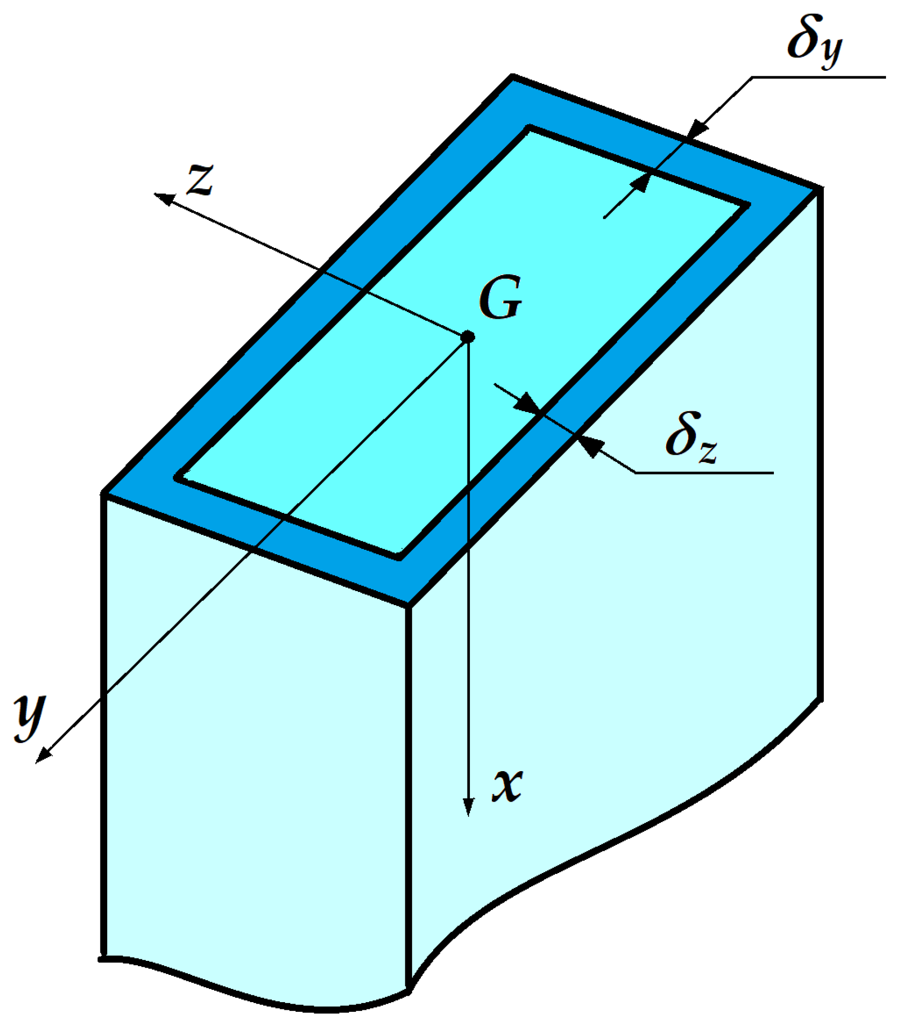
A beam with rectangular-hole section is considered, which is related to the tri-orthogonal reference system Gxyz (Figure 1). The beam is placed in air and submitted to electric heating at its base. The heat transfer is performed by conduction in the walls and by convection inside and outside the beam. The boundary condition at x = 0 corresponds to the temperature of the base which is measured experimentally (Dirichlet) and at x = L, the boundary condition corresponds to the equality between the heat transfer due to conduction and the heat transfer by convection from the cross-section surface to the surrounding air (Fourier).
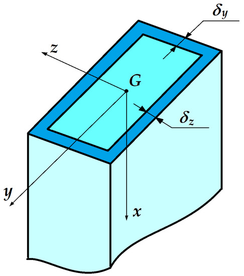
Figure 1.
Beam with rectangular-hole section.
All variables that can have an influence on the heat transfer in the beam with rectangular-hole section were are analysed in the afore-mentioned references [55,56,57,58,59,60].
In order to reduce the number of dimensionless variables , which will form the Model Law, the method of de-doubling the dimensions was used (here: de-doubling the lengths), according the principles given in [32,33].
The method of setting up the dimensionless variables were set, based on the MDA method indicated in [32,33] was already shown by the authors in the case of the beam with circular section [31]. Therefore, only the differences that occur at the beam with rectangular-hole section will be hereafter presented.
According to the principles of MDA, two variants of sets of the independent variables were selected, which constitute the elements of the corresponding matrices A:
- I.
- II.
It can be seen that the variables chosen in these two variants are directly related to the experimental measurements. Thus, by modifying these variables we can favorably influence the development of experimental measurements, having at our disposal a wide range of constructive solutions , respectively thermal loading of the model .
As shown in the case of a beam with a circular section [31], the variables, in the case of the rectangular hole beam, are divided into:
- Independent variables, included in matrix A, which are chosen a priori, both for the prototype and for the model;
- Dependent variables, contained in matrix B, which in turn correspond to the description:
- ○
- Heat transfer expressed by the experiment parameters of structures not covered with intumescent paints respectively ;
- ○
- Heat transfer for a theoretical analysis ;
- ○
- Similarity criteria (heat transfer correlations) related to this phenomenon,
- ○
- The behavior of structures covered with intumescent paint .
For the two analyzed variants, which in the opinion of the authors represent significant cases, these elements are summarized in the following tables (Table 2, Table 3, Table 4, Table 5, Table 6 and Table 7), both by specifying the variables together with their dimensions and by providing the related components of the Model Law.

Table 2.
Matrix A with the independent variables.

Table 3.
Part of matrix B with the quantities required by experiments (first part of matrix B).

Table 4.
Part of matrix B with the quantities required by theoretical calculations (first part of the quantities included in matrix B).

Table 5.
Part of B with the quantities required by theoretical calculations (second part of the quantities included in matrix).

Table 6.
Part of matrix B with the quantities required by the heat transfer correlations.

Table 7.
Matrix B for the properties of the intumescent paint properties.
As mentioned in a previous paper [48], the elements of the Model Law serve both to determine the magnitude of the variables related to the model based on a priori data for the prototype and to obtain the variable (or variables) of the prototype based on the measurement results, performed on the model, all these being the elements those constitute matrix B.
It should be mentioned here that the method developed in [32,33] to obtain the set of dimensionless variables from the Dimensional Set follows the next steps:
- the exponent of the dependent variable and the exponents of the independent variables are extracted from each line of matrices C–D; the first is equal to the unit and is extracted from matrix D and the others, which are zero or any real number, are extracted from matrix C;
- these exponents are forming an element of the Model Law, as indicated in the relation below and whose calculation is later shown in Section 4.3. in the case of the dependent variable (searched for the prototype):
- (see Equation (A51) from Appendix B);
- it can be observed that the dimensionless variable obtained (here, ) is equal to one and the dependent variable (here, ) is expressed as a function of the independent variables;
- then, all the involved variables are replaced by the scale factors, like , where subscript 1 refers to the prototype and subscript 2 to the model;
- finally, the first element of the Model Law is obtained, that is ;
- the other 50 elements of the Model Law were similarly calculated. In order to show the correctness of MDA and to validate the method, three elements were selected for the second variant.
4. Results
4.1. First Version of Independent Variables
In the first version, the following quantities are included (Table 2, Table 3, Table 4, Table 5, Table 6 and Table 7).
The corresponding elements of the Model Law to are presented in Appendix A (Equations (A1)–(A8)).
In this case the corresponding elements of the Model Law are determined and presented in Appendix B, to (Equations (A9)–(A28)):
where are defined , and are defined in Equations (1)–(3):
The corresponding elements of the Model Law are from to (see Appendix A, (Equations (A29)–(A41)).
In this case the corresponding elements of the Model Law are from to (see Appendix A, (Equations (A42)–(A50)).
4.2. Second Version of Independent Variables
In the second case, the following elements are included and presented in the Table 8, Table 9, Table 10, Table 11, Table 12 and Table 13.

Table 8.
The matrix A with the independent variables.

Table 9.
Part of matrix B including the quantities required for experiments (first part of matrix B).

Table 10.
Part of matrix B including the quantities required for theoretical calculations (first part of these quantities included in matrix B).

Table 11.
Part of matrix B including the quantities required for theoretical calculations (secon part of these quantities included in matrix B).

Table 12.
Part of matrix B including the quantities required by the heat transfer correlations.

Table 13.
Part of matrix B including the intumescent paint properties.
The corresponding elements of the Model Law are to (see Appendix B, (Equations (A51)–(A58)).
The corresponding elements of the Model Law are to (See Appendix B: (Equations (A59)–(A78)).
The mentioned dimensionless numbers , and have the same expressions (Equations (4)–(6)):
The corresponding elements of the Model Law are to (See Appendix B: (Equations (A79)–(A91)).
The corresponding elements of the Model Law are to (See Appendix B: Equations (A92)–(A100)).
One have to remark that from the tubular-rectangular sections, where generally the thicknesses of the tube in the two directions are different an identity of the expressions of the Model Law for and can be observed ( and ); for an expression derived from is obtained. Therefore the Model Law is valid also for rectangular-hole sections if the same scale is adopted as for and .
4.3. Model Law for the Second Version
In this case the set of independent variables was .
In order to illustrate how the elements of the Model Law can be applied in the study of the correlation between prototype and model, the following variables were selected:
- the heat supply in the prototype ;
- the cross-sectional area of the model ;
- the thickness of the paint layer applied on the model .
These variables are governed by the final relations:
and respectively
of the Model Law (see Equations (A51), (A52) respectively (A99) from Appendix B).
The size is related to the prototype, which cannot be determined by effective measurements, as all experiments were performed on the model. The sizes and belong to the model, and being dependent variables, they will rigorously result only by applying the Model Law. On the other hand, taking into account the set of independent variables, with a priori set sizes (prototype and model), their scale factors are also known from the beginning.
In order to determine , we start from the relationship , i.e., Equation (7), or more exactly from Equation (A51), Appendix B, where the definition of the scale factor is obtained in turn:
The cross-sectional area of the model results similarly from the Equation (8) for :
The thickness of the paint layer on the model will be obtained from the relationship for , i.e., Equation (9):
The case of the rectangular-hole beam, analyzed above, can be extended to bar structures of the same section, which is uniquely found in all resistance structures used in construction, such as industrial halls, gyms, shops, houses, living etc. Obviously, in this case homologous points and sections of the prototype and the model must be identified, in order to be able to find the homologous effect of the thermal stress applied to the model with that of the prototype based on the Model Law. The case of the square section is a particularly obvious case of the rectangular one.
In order to validate these results, an experimental setup described by the authors [54] consisting of a prototype and two models was designed, starting from the dimensions of an existing structural element (the supporting column of an industrial hall). Thus, for the prototype, made at 1:1 scale, a column segment with height was considered and, for the two models, made at 1:2 and 1:4 scales, respectively, segments with heights and, respectively .
Considering the combination of these structural elements, made at different scales, resulted three sets of prototypes-models, in our case (1:1 with 1:2); (1:1 with 1:4), respectively (1:2 with 1:4), all in two situations: unprotected, respectively thermally protected with layers of intumescent paints.
An original heating stand (with three-phase alternating current) was designed and physically made, with an original heating control and acquisition system, with the help of which it was monitored at the [°C] stabilized nominal temperature of the stabilized regime, the consumed electricity , as well as of the time necessary to reach this regime; repeating the previous step, in order to reach all the nominal temperatures of °C.
A stabilized temperature regime was considered to be achieved, when at the level of the last thermoresistance PT 100–402 (near the upper part of the tested structural element) the maximum temperature oscillations were observed for a minimum period of
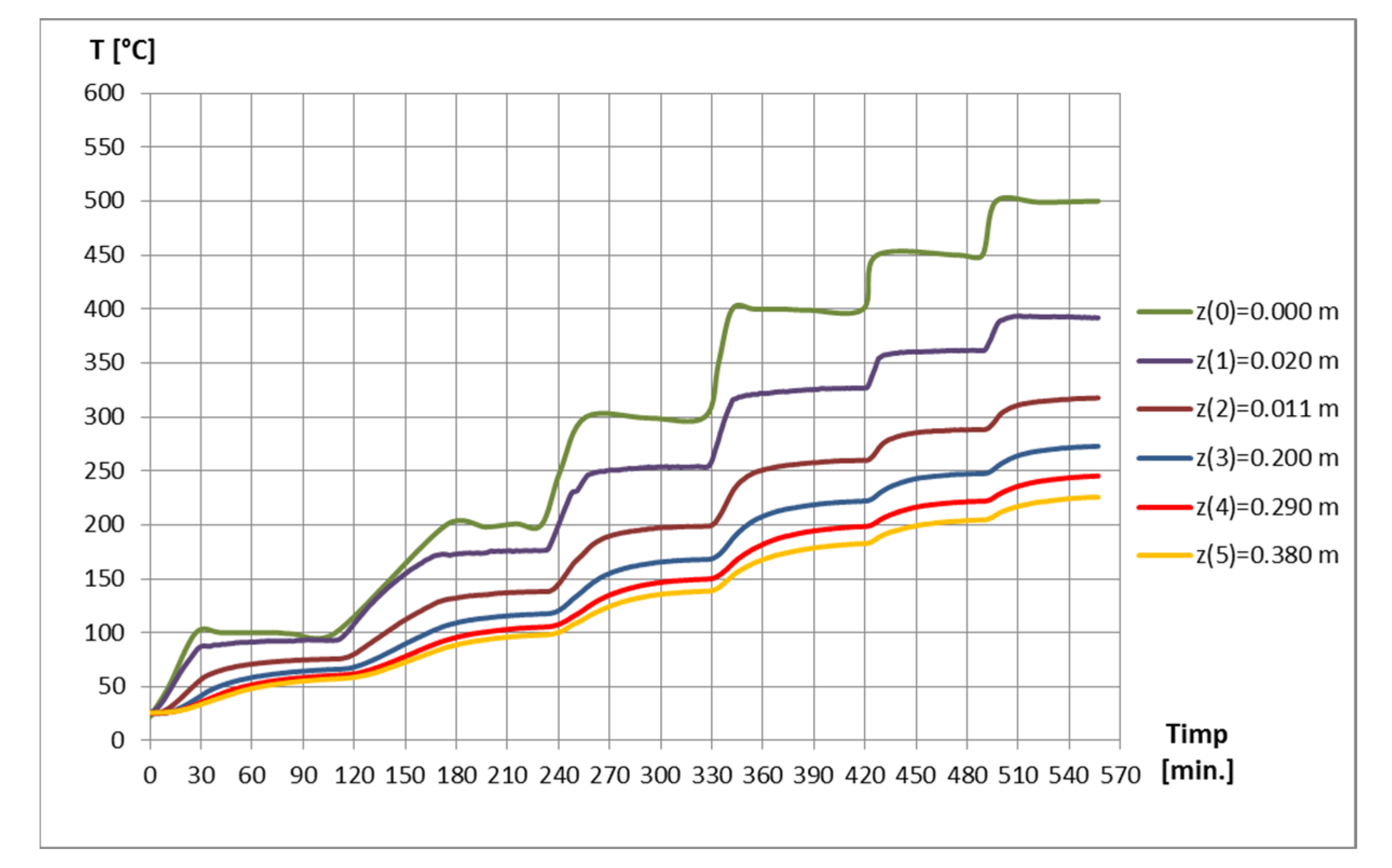
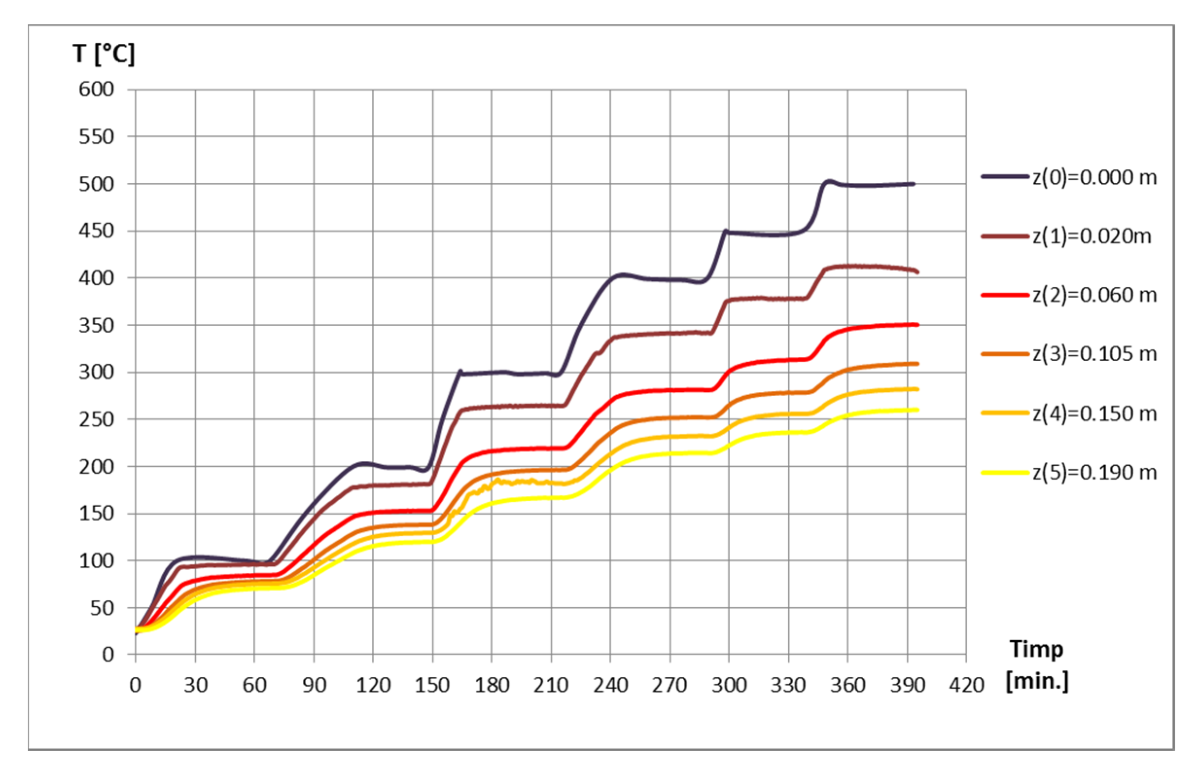
As illustration of the performed experimental investigations in the afore-mentioned research work [54], two diagrams are presented in Figure 2, Figure 3, Figure 4 and Figure 5, where one can remark the unitary predicted heating levels for the experimental validation of the Model Laws.
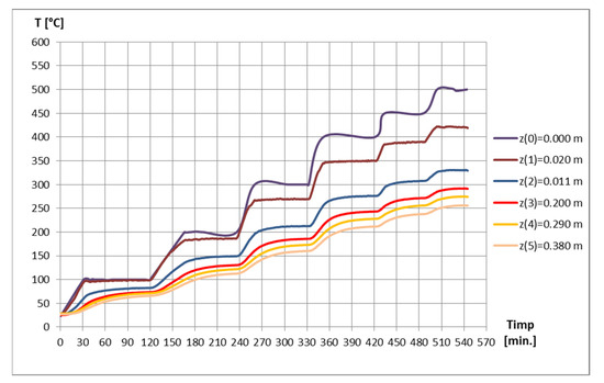
Figure 2.
The evolution of temperatures versus time in the unpainted prototype.
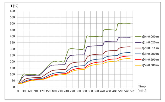
Figure 3.
The evolution of temperatures versus time in the painted prototype.
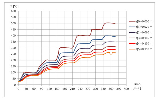
Figure 4.
The evolution over time of temperatures at the scale model 1:2 unpainted.
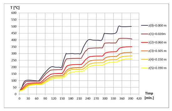
Figure 5.
The evolution over time of temperatures at the scale model 1:2 painted.
A very good agreement was obtained between the values based on measurements and those obtained with the help of the Model Law [54]. Based on the validation of these Model Laws, the authors will further extend the application of these laws to realized structures and other scales (for example to 1:5 or 1:10). This will allow the design and testing of very convenient models for simulating outbreaks of large real structures (e.g., industrial halls or multi-compartment or multi-floor buildings).
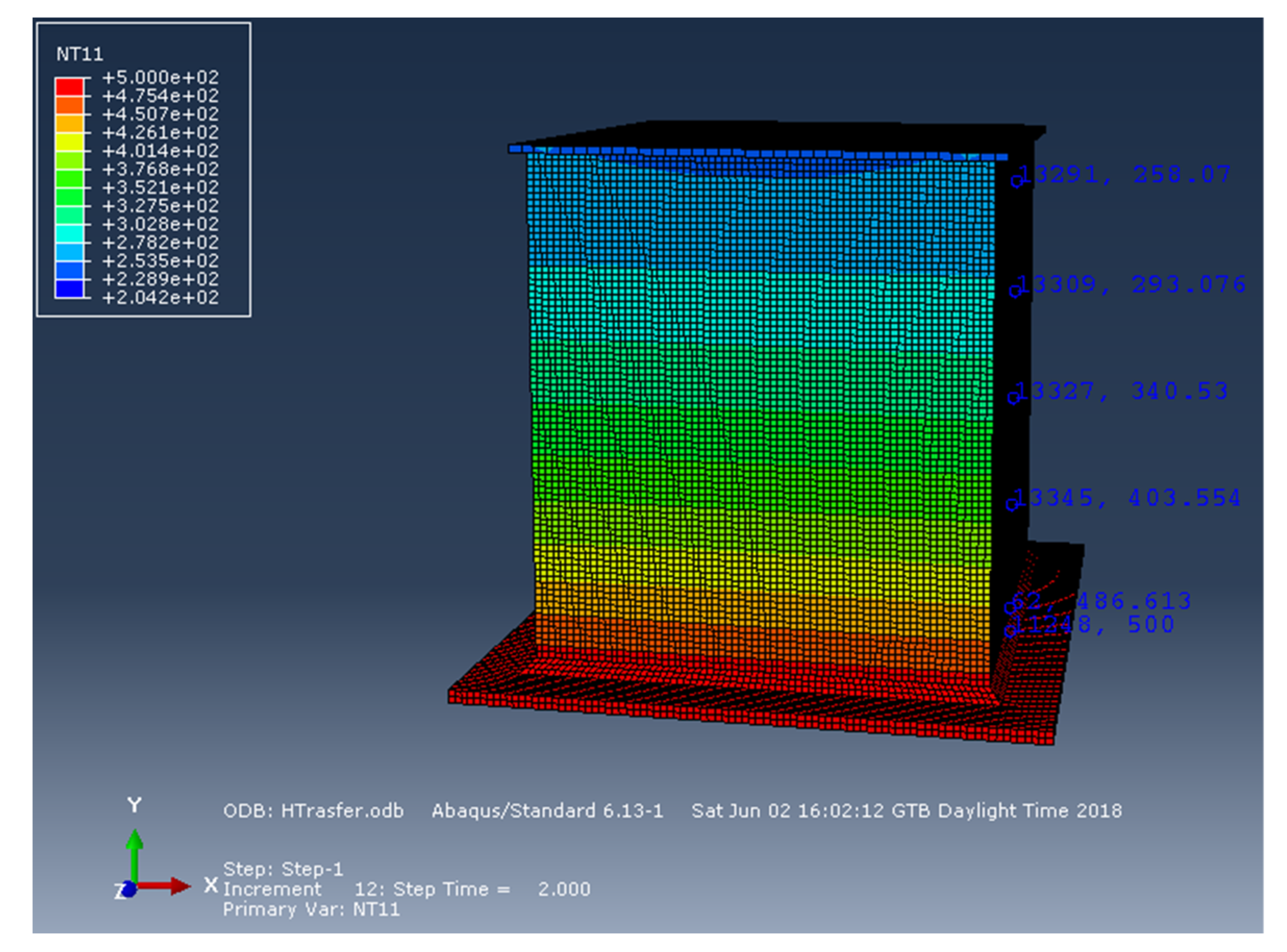
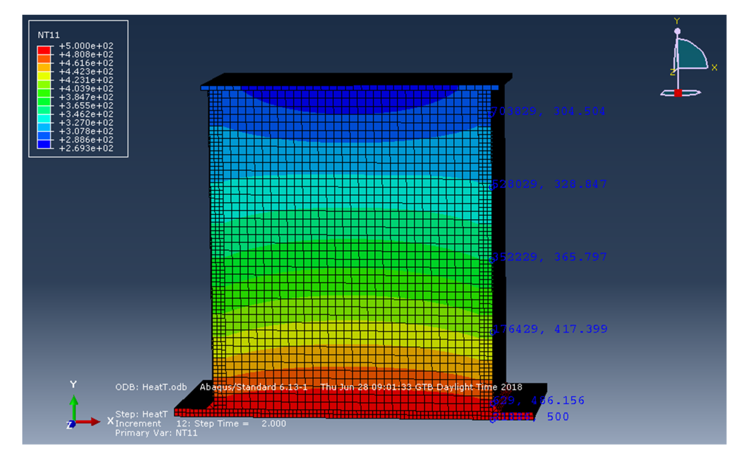
The numerical simulation of the thermal behavior was performed in ABAQUS, both for the structural elements performed at the 1:1 and 1:2 scales [58,60,61]. Figure 6, Figure 7, Figure 8 and Figure 9 show the modeling results of the uncovered prototype, respectively coated with heat-resistant paint [58]. Table 14 summarizes the main features of numerical modeling.
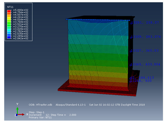
Figure 6.
Temperature distribution to the unpainted prototype, for TOn = 500 °C.
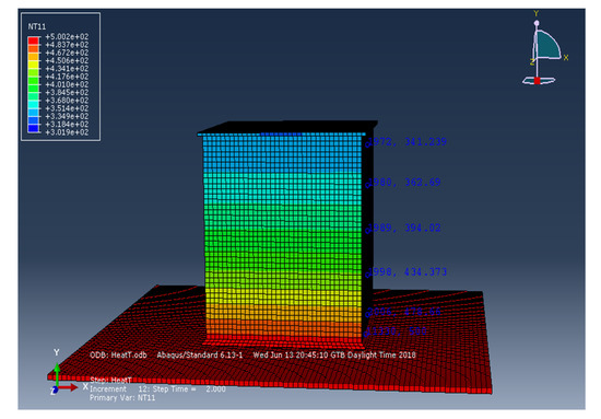
Figure 7.
Temperature distribution on the unpainted 1:2 scale model, for TOn = 500 °C.
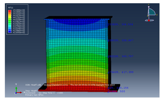
Figure 8.
Temperature distribution to the painted prototype, for TOn = 500 °C.
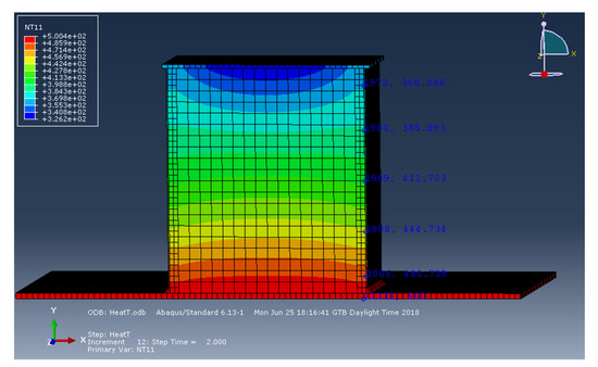
Figure 9.
Temperature distribution on the painted 1:2 scale model, for TOn = 500 °C.

Table 14.
The characteristics of the FEM models.
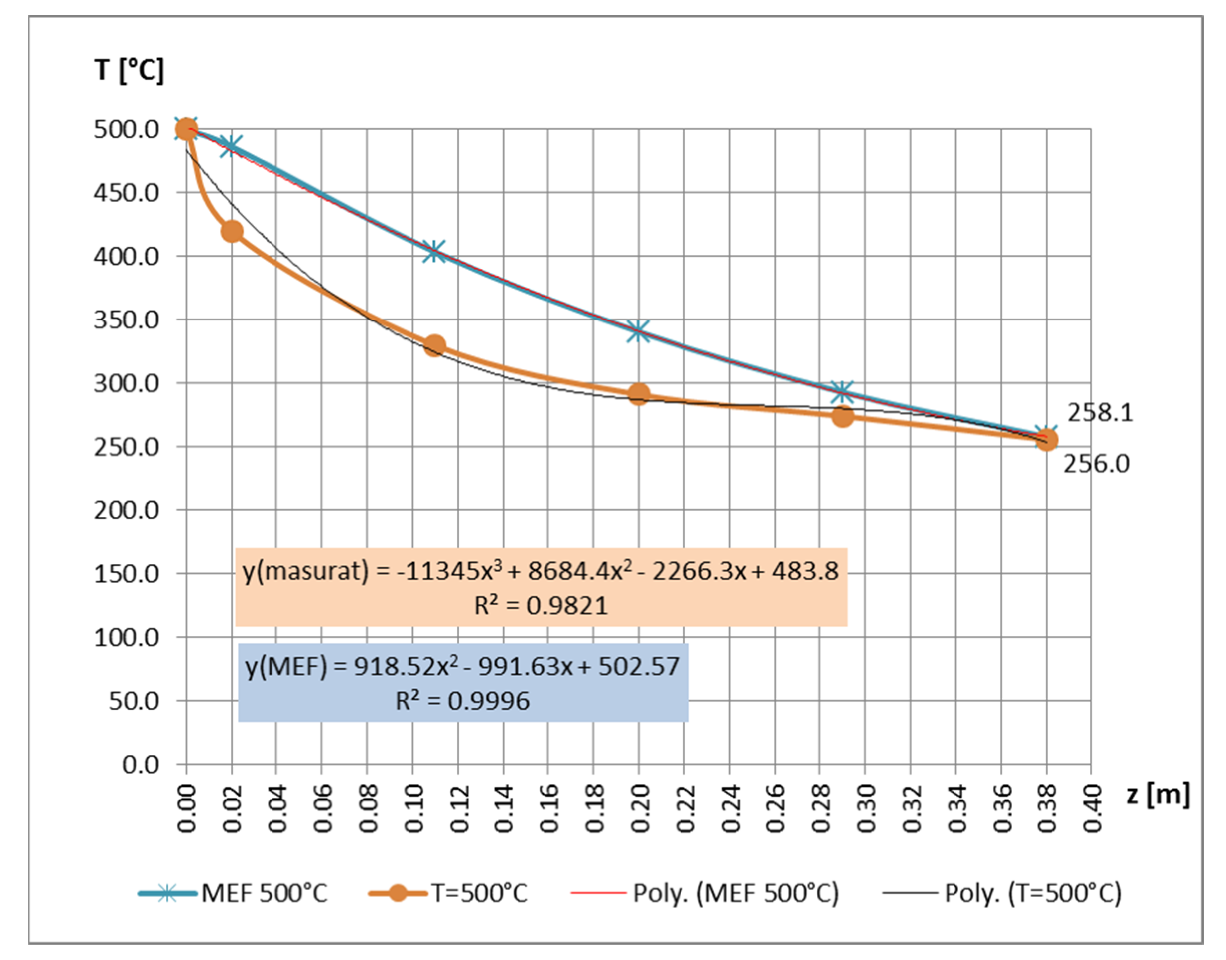
Figure 10 shows the temperature variation diagram based on the measurements, corresponding to the stabilized thermal regime, respectively the temperature diagram as a result of the numerical simulation, corresponding to the nominal temperature Ton = 500 °C. Given the fact that in the numerical simulation is not possible to obtain a stabilized thermal regime, but only a certain temperature in the heated area, another allure of the latter is observed. Obviously, for the thermally stabilized regime the allure would be much closer to the experimental curve. The figure also indicates the polynomial approximation functions of these curves.
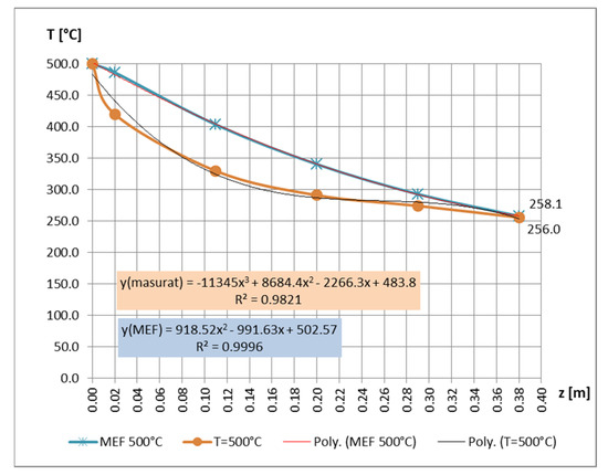
Figure 10.
Comparison of measurement results with those obtained with MEF on unpainted prototype [58].
5. Discussion
The dependent variable , which could not be determined by direct measurements on the prototype, results from the application of the Model Law.
The dependent variables, which are related to the model (here: and ), by applying the Model Law, provide the following facilities of the MDA, namely:
- In case of accepting the same length scale factor, the relationship can be ignored, but if more flexible models will be built, having different scale factors of cross sections, then by applying the relationship , this becomes possible, because the facilities offered by MDA;
- By considering identical thicknesses of intumescent paint on the prototype and model, the relationship can be ignored, but if different thicknesses of paint are desired, MDA allows us to do so;
- In this contribution, the authors offered the general cases of the rectangular-hole cross-sectional beam (with the complete set of the dimensionless variables), from where the particular cases of actual experiments were obtained;
We analyzed, for the two significant variants I and II, the complete sets of variables (so the totality of the elements/parameters) that can have any influence on this heat transfer.
6. Conclusions
A similar approach can be applied to the other dependent variables included in B matrices related to the theoretical analysis, the criteria, respectively the parameters of the intumescent paint (type of paint, layer thickness in the y or z direction etc).
If we take into account the existence in the set of independent variables, of both length () and shape factor , the definition of the model becomes even more general, i.e., we do not necessarily keep the geometric similarity; the model can have another shape of the cross section, but is it necessary to ensure a certain scale factor for . The authors’ experimental investigations [54], were able to provide a perfect validation of the Model Law deduced in this article.
If desired, instead of a geometric similarity of the cross sections (prototype-model), the variables (,) will help us to be able to design models with different wall thicknesses along the two coordinates , respectively to ensure different area model (,,), obviously with the strict compliance of the scales of these variables imposed by the elements of the Model Law.
The existence of among the elements of the A matrix also provides us with the opportunity (if necessary) to choose another material for the model in order to reduce the cost price of making and/or testing the model.
Considering of , respectively , as an independent variable, also ensures a great freedom in choosing the strategy of thermal stress of the model compared to that of the prototype. Considering as an independent variable gives the researcher the opportunity to choose a thermal regime as favorable as possible to load the model in relation to the prototype.
The case of the rectangular-hole beam, analyzed above, can be extended to bar structures of the same section, which is uniquely found in all resistance structures used in construction, such as industrial halls, gyms, shops, houses etc. Obviously, in this case homologous points and sections of the prototype and the model must be identified, in order to be able to find the homologous effect of the thermal stress applied to the model with that of the prototype based on the law of the model.
The existence of the exposure time to a certain thermal regime in the matrix A, brings another benefit of using/applying the Modern Dimensional Analysis to the track heat transfer in structures subjected to fires.
The experimental validation of the Model Law deduced in this article, was performed in conditions of maximum precision, taking into account the parameters followed, ie those significant in terms of the behavior of the thermal protection layer. By simulating a fire, with the help of a stand of their own design, the experimental measurements practically gave identical results to those of the Model Law.
A very good coincidence of the results was obtained, so the analytical results with the experimental ones were compared, proving the validity of the deduced Model Law.
Just considering these particular cases of the general Model Law, presented briefly in the paper, the advantages of the method described in [32,33] are important as compared to the Classical Dimensional Analysis. To the best knowledge of the authors, a similar approach of the heat transfer in bars of rectangular-tubular sections has not yet been performed. The ultimate goal of the detailed presentation of the advantages of MDA is to encourage engineers in the field to apply this very simple, safe and flexible method in their research.
Author Contributions
Conceptualization, I.S.; methodology, I.S. and D.Ș.; software, I.S., R.I.S. and K.J.; validation, D.Ș., I.S., R.I.S., K.J. and S.V.; formal analysis, I.S. and R.I.S.; investigation, I.S., R.I.S. and K.J.; resources, I.S.; data curation, D.Ș., I.S., R.I.S., K.J. and S.V.; original draft preparation, I.S., D.Ș. and S.V.; writing—review and editing, I.S., D.Ș. and S.V.; visualization, I.S., R.I.S. and K.J.; supervision, I.S., R.I.S. and K.J.; project administration, I.S. and R.I.S.; funding acquisition, I.S. and S.V. All authors have read and agreed to the published version of the manuscript.
Funding
This research received no external funding. The APC was funded by the Transilvania University of Brasov.
Institutional Review Board Statement
Not applicable.
Informed Consent Statement
Not applicable.
Data Availability Statement
Not applicable.
Conflicts of Interest
The authors declare no conflict of interest.
Nomenclature
| a | Thermal diffusivity (m2/s); |
| A | Area (m2); |
| Bi | Biot number; |
| Constant-pressure specific heat (J/ (°C kg)); | |
| Heat capacity (J/°C); | |
| F | Force (N); |
| Fo | Fourier number; |
| g | Gravitational acceleration (m/s2); |
| Gr | Grashof number; |
| l, L | Length (m); |
| Nu | Nusselt number; |
| P | Perimeter (m); |
| Pe | Péclet number; |
| Pr | Prandtl number; |
| Q | Heat (J); |
| Heat rate (W); | |
| Re | Reynolds number; |
| St | Stanton number; |
| t, T | temperature (°C); |
| V | volume (m3); |
| w | velocity (m/s); |
| -scale factor corresponding to the sizes indicated in the index. | |
| Greek symbols | |
| Convection heat transfer coefficient (W/(m2 °C)); | |
| Coefficient of volume expansion (°C)−1; | |
| Thickness (m); | |
| Variation; | |
| Dynamic viscosity (kg/ ms); | |
| Thermal conductivity (W/(m °C)); | |
| Kinematic viscosity (m2/s); | |
| Density (kg/m3); | |
| Shape factor (m−1); | |
| Time, shear stress (s, N/m2); | |
| Nabla operator. | |
| Subscripts | |
| x, y, z | Directions. |
Appendix A
Appendix B
References
- Schnittger, J.R. Dimensional Analysis in Design. J. Vib. Accoustic Stress Reliab. 1988, 110, 401–407. [Google Scholar] [CrossRef]
- Carinena, J.F.; Santander, M. Dimensional Analysis. Adv. Electron. Electron Phys. 1988, 72, 181–258. [Google Scholar]
- Canagaratna, S.G. Is dimensional analysis the best we have to offer. J. Chem. Educ. 1993, 70, 40–43. [Google Scholar] [CrossRef]
- Bhaskar, R.; Nigam, A. Qualitative Physics using Dimensional Analysis. Artif. Intell. 1990, 45, 73–111. [Google Scholar] [CrossRef]
- Romberg, G. Contribution to Dimensional Analysis. Ing. Arch. 1985, 55, 401–412. [Google Scholar] [CrossRef]
- Coyle, R.G.; Ballicolay, B. Concepts and Software for Dimensional Analysis in Modeling. IEEE Trans. Syst. Man Cybern. 1984, 14, 478–487. [Google Scholar] [CrossRef]
- Barr, D.I.H. Consolidation of Basics of Dimensional Analysis. J. Eng. Mech. 1984, 110, 1357–1376. [Google Scholar] [CrossRef]
- Remillard, W.J. Applying Dimensional Analysis. Am. J. Phys. 1983, 51, 137–140. [Google Scholar] [CrossRef]
- Martins, R.D.A. The Origin of Dimensional Analysis. J. Frankl. Inst. 1981, 311, 331–337. [Google Scholar] [CrossRef]
- Gibbings, J.C. A Logic of Dimensional Analysis. J. Physiscs A-Math. Gen. 1982, 15, 1991–2002. [Google Scholar] [CrossRef]
- Szekeres, P. Mathematical Foundations of Dimensional Analysis and the Question of Fundamental Units. Int. J. Theor. Phys. 1978, 17, 957–974. [Google Scholar] [CrossRef]
- Carlson, D.E. Some New Results in Dimensional Analysis. Arch. Ration. Mech. Anal. 1978, 68, 191–210. [Google Scholar] [CrossRef]
- Gibbings, J.C. Dimensional Analysis. J. Phys. A-Math. Gen. 1980, 13, 75–89. [Google Scholar] [CrossRef]
- Jofre, L.; del Rosario, Z.R.; Iaccarino, G. Data-driven dimensional analysis of heat transfer in irradiated particle-laden turbulent flow. Int. J. Multiph. Flow 2020, 125, 103198. [Google Scholar] [CrossRef]
- Alshqirate, A.A.Z.S.; Tarawneh, M.; Hammad, M. Dimensional Analysis and Empirical Correlations for Heat Transfer and Pressure Drop in Condensation and Evaporation Processes of Flow Inside Micropipes: Case Study with Carbon Dioxide (CO2). J. Braz. Soc. Mech. Sci. Eng. 2012, 34, 89–96. [Google Scholar] [CrossRef]
- Levac, M.L.J.; Soliman, H.M.; Ormiston, S.J. Three-dimensional analysis of fluid flow and heat transfer in single- and two-layered micro-channel heat sinks. Heat Mass Transf. 2011, 47, 1375–1383. [Google Scholar] [CrossRef]
- Nakla, M. On fluid-to-fluid modeling of film boiling heat transfer using dimensional analysis. Int. J. Multiph. Flow 2011, 37, 229–234. [Google Scholar] [CrossRef]
- Illan, F.; Viedma, A. Experimental study on pressure drop and heat transfer in pipelines for brine based ice slurry Part II: Dimensional analysis and rheological Model. Int. J. Refrig.-Rev. Int. Du Froid 2009, 32, 1024–1031. [Google Scholar] [CrossRef]
- Nezhad, A.H.; Shamsoddini, R. Numerical Three-Dimensional Analysis of the Mechanism of Flow and Heat Transfer in a Vortex Tube. Therm. Sci. 2009, 13, 183–196. [Google Scholar] [CrossRef]
- Asgari, O.; Saidi, M. Three-dimensional analysis of fluid flow and heat transfer in the microchannel heat sink using additive-correction multigrid technique. In Proceedings of the Micro/Nanoscale Heat Transfer International Conference, PTS A AND B. 1st ASME Micro/Nanoscale Heat Transfer International Conference, Tainan, Taiwan, 6–9 January 2008; pp. 679–689. [Google Scholar]
- Carabogdan, I.G.; Badea, A.; Brătianu, C.; Muşatescu, V.I. Methods of Analysis of Thermal Energy Processes and Systems; Ed. Tehn.: Bucharest, Romania, 1989. [Google Scholar]
- Baker, W.; Westine, P.S.; Dodge, F.T. Similarity Methods in Engineering Dynamics; Elsevier: Amsterdam, The Netherlands, 1991. [Google Scholar]
- Sedov, I.L. Similarity and Dimensional Methods in Mechanics; MIR Publisher: Moscow, Russia, 1982. [Google Scholar]
- Șova, M.; Șova, D. Thermotechnics, VL.II.; Transilvania University Press: Brasov, Romania, 2001. [Google Scholar]
- Zierep, J. Similarity Laws and Modelling; Marcel Dekker: New York, NY, USA, 1971. [Google Scholar]
- Chen, W.K. Algebraic Theory of Dimensional Analysis. J. Frankl. Inst. 1971, 292, 403–409. [Google Scholar] [CrossRef]
- Barenblatt, G.I. Dimensional Analysis; Gordon and Breach: New York, NY, USA, 1987. [Google Scholar]
- Bridgeman, P.W. Dimensional Analysis; Yale University Press: New Haven, CT, USA, 1922; (Reissued in paperbound in 1963). [Google Scholar]
- Buckingham, E. On Physically Similar Systems. Phys. Rev. 1914, 4, 345. [Google Scholar] [CrossRef]
- Quintier, G.J. Fundamentals of Fire Phenomena; John Willey & Sons: Hoboken, NJ, USA, 2006. [Google Scholar]
- Gálfi, B.-P.; Száva, I.; Șova, D.; Vlase, S. Thermal Scaling of Transient Heat Transfer in a Round Cladded Rod with Modern Dimensional Analysis. Mathematics 2021, 9, 1875. [Google Scholar] [CrossRef]
- Szirtes, T. The Fine Art of Modelling. SPAR J. Eng. Technol. 1992, 1, 37. [Google Scholar]
- Szirtes, T. Applied Dimensional Analysis and Modelling; McGraw-Hill: Toronto, ON, Canada, 1998. [Google Scholar]
- Trif, I.; Asztalos, Z.; Kiss, I.; Élesztős, P.; Száva, I.; Popa, G. Implementation of the Modern Dimensional Analysis in Engineering Problems-Basic Theoretical Layouts. Ann. Fac. Eng. Hunedoara 2019, 17, 73–76. [Google Scholar]
- Phatak, D.R.; Dhonde, H.B. Dimensional analysis of reinforced concrete beams subjected to pure torsion. J. Struct. Eng. 2003, 129, 1559–1563. [Google Scholar] [CrossRef]
- Alhama, F.; Madrid, C.N. Discriminated dimensional analysis versus classical dimensional analysis and applications to heat transfer and fluid dynamics. Chin. J. Chem. Eng. 2007, 5, 626–631. [Google Scholar] [CrossRef]
- Olsen, Z.J.; Kim, K.J. Characterizing the transduction behavior of ionic polymer-metal composite actuators and sensors via dimensional analysis. Smart Mater. Struct. 2002, 31, 025014. [Google Scholar] [CrossRef]
- Loreti, G.; Facci, A.L.; Peters, T.; Ubertini, S. In-depth characterization through dimensional analysis of the performance of a membrane-integrated fuel processor for high purity hydrogen generation. Int. J. Hydrog. Energy 2022, 47, 2442–2460. [Google Scholar] [CrossRef]
- Hosseini, S.; Mousavi, A.; Monjezi, M. Prediction of blast-induced dust emissions in surface mines using integration of dimensional analysis and multivariate regression analysis. Arab. J. Geosci. 2022, 15, 163. [Google Scholar] [CrossRef]
- Lv, J.; Zhang, X.; Liu, S.; Lu, H.; Ma, Y.; Hu, L.H. Flame morphology of horizontal jets under sub-atmospheric pressures: Experiment, dimensional analysis and an integral model. Fuel 2022, 307, 121891. [Google Scholar] [CrossRef]
- Esmaeilian, A.; O’Shea, K.E. Application of dimensional analysis in sorption modeling of the styryl pyridinium cationic dyes on reusable iron based humic acid coated magnetic nanoparticles. Chemosphere 2022, 286 Pt 2, 131699. [Google Scholar] [CrossRef] [PubMed]
- Száva, I.; Szirtes, T.; Dani, P. An Application of Dimensional Model Theory in The Determination of the Deformation of a Structure. Eng. Mech. 2006, 13, 31–39. [Google Scholar]
- Yao, S.; Yan, K.; Lu, S.; Xu, P. Prediction and application of energy absorption characteristics of thinwalled circular tubes based on dimensional analysis. Thin-Walled Struct. 2018, 130, 505–519. [Google Scholar] [CrossRef]
- Ferro, V. Assessing flow resistance law in vegetated channels by dimensional analysis and self-similarity. Flow Meas. Instrum. 2019, 69, 101610. [Google Scholar] [CrossRef]
- Langhaar, H.L. Dimensional Analysis and Theory of Models; John Wiley & Sons Ltd.: New York, NY, USA, 1951. [Google Scholar]
- Kivade, S.B.; Murthy, C.S.N.; Vardhan, H. The use of Dimensional Analysis and Optimisation of Pneumatic Drilling Operations and Operating Parameters. J. Inst. Eng. India Ser. D 2012, 93, 31–36. [Google Scholar] [CrossRef]
- Pankhurst, R.C. Dimensional Analysis and Scale Factor; Chapman & Hall Ltd.: London, UK, 1964. [Google Scholar]
- Khan, M.A.; Shah, I.A.; Rizvi, Z.; Ahmad, J. A numerical study on the validation of thermal formulations towards the behaviours of RC beams. Sci. Mater. Today Proc. 2019, 17, 227–234. [Google Scholar] [CrossRef]
- Yen, P.H.; Wang, J.C. Power generation and electrical charge desnity with temperature effect of alumina nanofluids using dimensional analysis. Energy Convers. Manag. 2009, 186, 546–555. [Google Scholar] [CrossRef]
- Lawson, R.M. Fire engineering design of steel and composite buildings. J. Constr. Steel Res. 2001, 57, 1233–1247. [Google Scholar] [CrossRef]
- Al-Homoud, M.S. Performance characteristics and practical applications of common building thermal insulation materials. Build. Environ. 2005, 40, 353–366. [Google Scholar] [CrossRef]
- Papadopoulos, A.M. State of the art in thermal insulation materials and aims for future developments. Energy Build. 2005, 37, 77–86. [Google Scholar] [CrossRef]
- Wong, M.B.; Ghojel, J.I. Sensitivity analysis of heat transfer formulations for insulated structural steel components Fire. Saf. J. 2003, 38, 187–201. [Google Scholar] [CrossRef]
- Noack, J.; Rolfes, R.; Tessmer, J. New layerwise theories and finite elements for efficient thermal analysis of hybrid structures. Comput. Struct. 2003, 81, 2525–2538. [Google Scholar] [CrossRef]
- Bailey, C. Indicative fire tests to investigate the behaviour of cellular beams protected with intumescent coatings. Fire Saf. J. 2004, 39, 689–709. [Google Scholar] [CrossRef]
- Bahrami, A.; Mousavi Anijdan, S.H.; Ekrami, A. Prediction of mechanical properties of DP steels using neural network model. J. Alloys Compd. 2005, 392, 177–182. [Google Scholar] [CrossRef]
- Yang, K.-C.; Chen, S.-J.; Lin, C.C.; Lee, H.H. Experimental study on local buckling of fire-resisting steel columns under fire load. J. Constr. Steel Res. 2005, 61, 553–565. [Google Scholar] [CrossRef]
- Munteanu, I.R. Investigation Concerning Temperature Field Propagation along Reduced Scale Modelled Metal Structures. Ph.D. Thesis, Transilvania University of Brasov, Brasov, Romania, 2018. [Google Scholar]
- Dani, P. Theoretical and Experimental Study of Heat-Field Propagation through Multi-Layer Fire-Protection on Stress-, and Strain-State of Metallic Structures. Ph.D. Thesis, Transilvania University of Brasov, Brasov, Romania, 2011. [Google Scholar]
- Száva, I.R.; Șova, D.; Dani, P.; Élesztős, P.; Száva, I.; Vlase, S. Experimental Validation of Model Heat Transfer in Rectangular Hole Beams Using Modern Dimensional Analysis. Mathematics 2022, 10, 409. [Google Scholar] [CrossRef]
- Turzo, G.; Száva, I.R.; Gálfi, B.P.; Száva, I.; Vlase, S.; Hoța, H. Temperature distribution of the straight bar, fixed into a heated plane surface. Fire Mater. 2018, 42, 202–212. [Google Scholar] [CrossRef]
Publisher’s Note: MDPI stays neutral with regard to jurisdictional claims in published maps and institutional affiliations. |
© 2022 by the authors. Licensee MDPI, Basel, Switzerland. This article is an open access article distributed under the terms and conditions of the Creative Commons Attribution (CC BY) license (https://creativecommons.org/licenses/by/4.0/).

