A Complex Network-Based Airspace Association Network Model and Its Characteristic Analysis

Abstract

As airspace congestion becomes more and more serious, it not only affects the efficiency and quality of aviation activities, but also poses a greater safety hazard. For in-depth exploration of the airspace network, a new airspace association network that differs from the traditional aviation approach of organizing the airspace into a network of sectors based on aircraft traffic flow is proposed. By judging the relationship between the size and location of the airspace and other properties, the establishment of an association network provides new ideas for airspace conflict detection and other aerial tasks. The three key factors of airspace use conflict were extracted and quantified, then the Analytic Hierarchy Process (AHP) was used to assign weights to basic symmetric operators corresponding to three factors to calculate the final airspace correction degree, which reveals the magnitude of correlation degree between the airspace caused by the combined action of the above three factors. Finally, an airspace association network model was established according to the association degree, using basic symmetric operators to explore the general symmetry and network characteristics in real-world airspace association networks, and the feature indices, such as degree, strength, average correlation, clustering coefficient, and structure information entropy of the network, are proposed. The results show that the nodes with higher node degree and node association strength are often key nodes in the network, and the areas with higher average association degree and clustering coefficient are often more prone to airspace conflicts. At the same time, it was also verified that the safety distance between airspace has the greatest impact on the characteristics of the airspace association network.

1. Introduction

With the rapid development of the civil aviation industry in various countries in the world, global air traffic continues to maintain a high-speed growth trend. At the same time, the air traffic congestion and airspace conflict caused by it are becoming more and more serious. It not only seriously affects aviation economic benefits and service quality, but also causes huge potential safety hazards. Air traffic control is a key role in ensuring the safety, smoothness and efficiency of air traffic, improving the efficiency of air traffic control is an effective way to solve the problem. In the future, the trend of integrated joint operations will make airspace management tasks more important. As the basic unit of traffic control services, airspace carries many important tasks such as aircraft flight, weapon and equipment coordination, and route planning. Faced with the needs of users to use airspace, airspace resources are more precious and tense. Therefore, it is of far-reaching significance to conduct in-depth research on the operation mechanism and hierarchical structure of airspace [1].

The generalized concept of airspace refers to all the space above the land, which has been a relatively vague and complex concept for a long time due to the different defining perspectives and special usage attributes [2]. The airspace mentioned in this article refers to the task (predetermined) airspace: in order to meet the airspace users’ needs for different airspace, marked by obvious landmarks or navigation stations, a certain range of space is delineated according to the needs of flight training and operations. For the basic concepts and attributes of airspace, Bauranov, A made a more detailed analysis and summary in the literature from safety-related factors, social factors, system factors and aircraft factors [3]. In terms of airspace operation mechanisms, the airspace management in the United States and some European countries has always been relatively loose, and airlines can choose and decide routes and flights without government approval. In comparison, since 80% of the airspace is controlled by the military [4], China’s airspace management and operation mechanism is relatively complex and rigid. All require approval from at least 3–4 management units, reducing air traffic flow and operational efficiency. After the airspace is officially put into use, airspace users must strictly conduct air activities within the scope of the applied airspace.

Through data research, it was found that optimizing the operating mechanism and opening the authority to use airspace can improve the efficiency of use. However, for the sake of safety and confidentiality, most national policies have stricter regulations on the operating mechanism of the airspace, and there is not much room for opening up and improving the airspace utilization mechanism. Therefore, current research on airspace mainly focuses on airspace planning [5,6] and capacity assessment [7,8,9]. These studies can optimize the structure and operation mechanism of a single or a few airspace to a certain extent, but research on the relationship and hierarchy within the airspace group composed of multiple airspace is still insufficient. However, air traffic control is a holistic work, and the interaction between airspace is also complex and diverse. Therefore, it is necessary to consider multiple airspace objects from the overall perspective, build an airspace network, and conduct analysis and research from the system level.

Airspace network construction is a complex and systematic problem. In 2002, Zhang Jiqiang [10] expressed the network node as the starting sector to the ending sector (which may contain multiple airspace sectors) that the aircraft traverses in a specified time interval and introduced the concept of network into airspace modeling for the first time, but it is different from the airspace. The actual dynamics and continuity are not well matched. In 2014, Gurtner et al. [11] used grid community detection to analyze and model European airspace. The research results provided certain guidance and help for the use and division of European airspace as a whole, but they did not establish a network with airspace as a node. The literature [12,13,14,15,16,17] proposes that the sector is used as a node, and the flow relationship (number of flights) between sectors is used as an edge, and the network structure of the control sector is initially established. It provides theoretical guidance for alleviating airspace use conflicts, reducing flight delays and optimizing airspace resource management. It can be seen that the above-mentioned research results have been relatively abundant, but most of the airspace network nodes currently researched are based on sectors, and the edges are set according to the flight flow relationship between sectors. This airspace sector network can reflect the sector’s operating status, flight handover frequency, controller communication and overall airspace structural characteristics to a certain extent, but a sector often contains multiple mission airspace, and some air activities such as airspace conflicts detection needs to pay more attention to the relationship between airspace individuals at the level of natural attributes, so it is necessary to establish an association network with airspace as a node to reflect the relationship between airspace.

The airspace association network is essentially based on the closeness of the relationship between airspace nodes in the dimensions of location, size and use time. The biggest difference from the airspace sector network is that the connection of the sector network reflects the flow relationship, while the node connection of the airspace association network reflects whether there is an association relationship. Regarding the problem of airspace correlation network construction, one is to assign reasonable and effective weights to multiple impact indicators between airspace; the factors are aggregated and combined according to their interrelated influences and affiliations to form a multi-level analytical structure model and calculate the final target value airspace correlation degree. Airspace correlation degree is an important indicator to measure the relationship between airspace. It is calculated by combining influence factors in different dimensions between airspace according to the combination of interrelated influences. Whether the spatial correlation degree exists or not indicates whether there is a correlation between airspace, and the value of the airspace correlation degree indicates the size of the correlation degree between airspace. The second is to choose an appropriate network construction method to ensure that the constructed network can provide information to aid airspace management decision making.

For the problem of assigning weights to indicators, the solutions are mainly studied from the perspectives of subjective weighting and objective weighting. The subjective weighting method is more typical of the Analytic Hierarchy Process [18] (AHP) proposed by American operations researcher Sati, a professor at the University of Pittsburgh in the early 1970s. This systematic method includes decomposing the target into multiple targets or criteria. The final goal is then determined through qualitative indicators and fuzzy quantitative methods. There are two main types of objective weighting methods: principal component analysis [19] and entropy weighting. The principal component analysis [20] method mainly converts a number of highly correlated indicators into a few comprehensive indicators through dimensionality reduction, so as to achieve the goal of simplifying the problem through mathematical transformation. The entropy weight method [21] uses the entropy value to judge the degree of dispersion of an index, so as to judge the greater the influence (weight) of the index on comprehensive evaluation and use the information entropy tool to calculate the weight of each index and provide a basis for comprehensive evaluation. Three indicators are involved in this paper. The correlation between the indicators is not strong and the discreteness is difficult to judge. Therefore, the method of objective weighting was excluded, and the analytic hierarchy process of subjective weighting was finally selected.

Regarding selecting a method for network construction, developments in the field of complex networks have provided mature systems to support the construction of an airspace association network model. Zhou Ren [22] reviewed the research on topology recognition of complex networks in recent years and discussed the steps of network topology recognition. Cao, L.X. [23], based on rough set theory, defines uncertainty in complex networks and proposes key concepts. Pluhacek, M. [24] first proposed the use of multi-swarm particle swarm algorithm to create complex networks. Runhu Tian [25] established an analysis model of target nodes in complex networks and explored the search mechanism of target nodes in complex networks. Wu, Y.P. [26] studied the relationship between the fractal dimension and the robustness of different types of complex networks from the perspectives of network structure and network scale, providing a new perspective for evaluating the robustness of complex networks. Wen, T. [27] proposed the information dimension of weighted complex networks to help reveal the important properties of complex networks: fractal and self-similarity. Hong Zhang [28] used the trace of adjacency matrix and the centrality of the complex network to conduct quantitative and qualitative analysis of complex networks. Lintao L. [29] proposed a multi-scale network community detection algorithm based on fractal feature evolution to solve the problem of community discovery in dynamic complex networks. Dai, J.C. [30] proposed a structured compressed sensing method for global reconstruction of complex network topology by analyzing and extracting the basic features of weightless and undirected networks. The main research methods of complex networks are based on the theories and methods of graph theory and have achieved gratifying results, which have been widely used in many scientific fields. For example, the foreign exchange [31] market network was established by calculating the correlation of transaction information; the nervous system [32] is a network formed by the interconnection of nerve cells through nerve fibers; and computer networks [33] can be regarded as computers that autonomously work and communicate with each other through a communication media network of connections. In addition, it also involves many fields, including logistics transportation [34,35], urban transportation [36,37,38] and information supply [39,40], etc., showing strong application potential and theoretical advantages. At present, more attention is paid to exploring the controllability and evolution of complex networks; that is, how to control complex networks and predict the future development trend of networks. In this field, several scholars such as Yali Zhang [41], Li, K. [42] and Chakraborty [43] have explored the subject qualitatively and quantitatively. At the same time, Chakraborty took the lead in proposing the evolution of finite-size complex networks with constrained chain addition. It has very important theoretical significance and practical value. In the research on symmetry problems, complex networks are also closely related to it. More and more studies have shown that real-world networks are far from strictly symmetrical networks. Therefore, with real-world networks, as with any entity characterized by imperfections, it is necessary to develop more general symmetry in a complex network, which also provides new ideas for solving symmetry problems [44,45]. Because complex network theory has obvious advantages in research and application in this field with its mature theoretical system, this paper chooses to use complex network theory as the construction tool of the airspace association network.

Based on the above analysis, this paper proposes a method to calculate the airspace correlation degree through the weighted index of the AHP method to obtain the airspace correlation relationship and uses the complex network theory to establish the network and analyze the network characteristics. The key factors of airspace conflict are extracted and quantified into three corresponding mathematical indicators: time correlation, spatial correlation and family correlation, and then the analytic hierarchy process method is used to assign different weights to the three indicators and combine the three indicators as the degree of correlation between spaces. Then, an association network is constructed according to the relationship between spatial domains, and five network characteristics are extracted to analyze the network using the complex network correlation theory. This new airspace association network removes the traditional sector network’s method of establishing relationships with flight flow. For the first time, the relationship between airspace is presented in a visual way, which can provide airspace controllers with first-hand information to assist decision making. At the same time, the introduction of complex network theory has deepened research on the qualitative and quantitative aspects of airspace correlation networks and provided guidance and a basis for future airspace structure design and airspace intelligent resolution.

2. Basic Symmetric Operator Definition

This paper mainly considers the time range of the airspace, the Euclidean distance between the airspace and the consanguinity relationship between the airspace. By summarizing the law of the influence of each operator on the correlation between spatial domains, and choosing an appropriate method to express the operator, the basic operator has a certain symmetry. In the same research object (mission airspace pair), the parameters involved are symmetrical and equal. The concepts of time correlation ($\tau$), spatial correlation ($\omega$) and family relationship ($\psi$) are introduced.

2.1. Airspace Time Correlation $\tau$

The time correlation degree reflects the degree of conflict between the two airspace in the time dimension. When planning the use of airspace, each airspace has a pre-set time of use, and the length of the time horizon is expressed as $t$. If there is conflict between airspace $i$ and airspace $j$ in the time dimension, the time of conflict between airspace is represented by $t_{ij}$. At the same time, the safety margin time between airspace is set as $t_s=0.25 \mathrm{h}$, the average of the sum of the conflict time between airspace and the safety margin time is set as the airspace association time $t_c=\left(t_{ij}+t_s\right)/2$, the mean of the sum of airspace usage times is set as the airspace pair average usage time $\overline{t_{ij}}=\left(t_i+t_j\right)/2$. The ratio of the airspace association time to the airspace pair average usage time is defined as the time correlation degree, which represents the time association degree between airspace:

$${\tau }_{ij}={\tau }_{ji}=\frac{t_c}{\overline{t_{ij}}}=\frac{t_{ij}+t_s}{t_i+t_j}$$

(1)

For example, the usage time of airspace $A$ is 08:00–10:00 on 25 December 2020, $t_A=2$ and the usage time of airspace $B$ is 09:00–12:00 on 25 December 2020, $t_B=3$. The two-mission airspace conflict time period is 09:00–10:00, $t_{AB}=1$, the time correlation of the two airspace is ${\tau }_{AB}=\left(1+0.25\right)/5=0.25$. By analyzing the overlap ratio of the time periods used in the airspace, the time correlation degree between the airspace is calculated, and the correlation influence degree between the airspace in the time dimension is obtained.

2.2. Airspace Spatial Correlation $\epsilon$

Each airspace has its own shape and size; the spatial correlation degree reflects the degree of conflict between two airspace in a three-dimensional space. Since it is difficult to find the center of the airspace in the three-dimensional space, the method of dimensionality reduction is adopted. First, the target airspace is orthographically projected [46,47,48,49] to the two-dimensional plane (as shown in Figure 1), and the coordinates of the center point of the airspace $z_i$ on the two-dimensional plane are calculated. According to the upper and lower limit heights of the airspace, the height center value of the airspace $\overline{h_i}$ is obtained, and the coordinates of the center point of the airspace $g_i=\left(z_i,\overline{h_i}\right)$ are obtained by combination.

The average distance from the center point of each airspace to the edge of the airspace is set as $\overline{d_i}$, the center coordinates of airspace $A$ and airspace $B$ are concatenated to form the vector $\overrightarrow{AB}$, and the modulus value of the vector $\overrightarrow{g_A{g}_B}$ is used as the center distance $d_{AB}$, then the average use distance $\overline{d_{ir}}=\left(\overline{d_i}+\overline{d_r}\right)/2$ is calculated for the airspace pair. At the same time, considering the safety distance $s$ between airspace ensures the safety of the airspace; the spatial correlation degree of the airspace is defined as follows:

$$D_{ir}=\left|\overrightarrow{g_i{g}_r}\right|-\left(\overline{d_i}+\overline{d_r}\right)-s,{\epsilon }_{ir}=\left\{\begin{array}{cc}\frac{D_{ir}}{\overline{d_{ir}}}=\frac{\left|\overrightarrow{g_i{g}_r}\right|-\left(\overline{d_i}+\overline{d_r}\right)-s}{\overline{d_{ir}}}& D_{ir}<0\\ 0& D_{ir}\ge 0\end{array}\right.$$

(2)

In Formula (2), $D_{ir}$ represents the redundancy distance between two airspace. According to the relevant regulations of ICAO Doc 8168 Aircraft Operation Volume 1—Flight Procedures [50], the safe distance between airspace is generally taken as $s=10 \mathrm{km}$$\left(5\mathrm{NM}\right)$. The ratio of the average distance between the centers of the airspace and the edge and the redundancy distance between the airspace is defined as the spatial correlation degree between the airspace. From this, the degree of correlation between the airspace in the spatial dimension is obtained.

2.3. Airspace Family Relationship $\psi$

According to the inclusion relationship of airspace, the airspace can be preliminarily divided into parent–child airspace, sibling airspace and general airspace by imitating the kinship relationship in biology. In this paper, the spatial domain is coded with the help of the grid coding tool GeoSOT, and then the level and inclusion relationship are judged by the difference in the number of coding bits.

GeoSOT [51,52,53,54] is a grid system divided according to the quadtree, and its core idea is to logically extend the grid of integer “degree” and integer “minute”, so that the grid has integer characteristics. At the same time, a global quadtree grid structure ranging from the entire earth to centimeter-level patches is relatively fully realized. The area ratio of the parent–child patches between the upper and lower levels of the grid is roughly 4:1, and there is a consistent aggregation feature among the major gauge geographic grids in the world. In the way of grid division, in order to ensure that the next-level patch can be divided into four groups on the basis of the previous-level patch, the generated grid is encoded as an integer, and the earth’s surface is expanded three times. The corresponding relationship between the patches and scales at each level of GeoSOT is shown in

Table 1. Corresponding relationship between GeoSOT levels and scales.

Level	Grid Size	Approximate Size Near the Equator	Level	Grid Size	Approximate Size Near the Equator
G	512°		17	16″	512 m
1	256°		18	8″	256 m
2	128°		19	4″	128 m
3	64°		20	2″	64 m
4	32°		21	1″	32 m
5	16°		22	1/2″	16 m
6	8°	1024 km	23	1/4″	8 m
7	4°	512 km	24	1/8″	4 m
8	2°	216 km	25	1/16″	2 m
9	1°	128 km	26	1/32″	1 m
10	32′	64 km	27	1/64″	0.5 m
11	16′	32 km	28	1/128″	25 cm
12	8′	16 km	29	1/256″	12.5 cm
13	4′	8 km	30	1/512″	6.2 cm
14	2′	4 km	31	1/1024″	3.1 cm
15	1′	2 km	32	1/2048″	1.5 cm
16	32″	1 km

.

After completing the airspace grid coding work, if the level precision is different, but the coding at the same level is equal, it means that there is a parent–child relationship; if the level precision is the same, the parent level grid coding is also the same, and if the child level coding is different, it means that it is a sibling relationship; other airspace are general airspace. The family relationship of the airspace is defined here, and the corresponding values are shown in

Table 2. Classification of consanguinity correlation degree.

Family Relationship	Family Relationship Degree
Parent–child airspace	1
Sibling airspace	0–1
General airspace	0

:

(1)

Parent–child airspace: If the large airspace contains multiple small airspace, the small airspace is the child airspace, and the large airspace is the parent airspace;

(2)

Sibling airspace: If a large airspace contains multiple small airspace, the small airspace is the sibling airspace;

(3)

General airspace: All other airspace, except the parent–child airspace and the sibling airspace, are general airspace.

3. Establishment of Airspace Correlation Function Based on Analytic Hierarchy Process (AHP)

The degree of correlation between airspace needs to comprehensively consider multiple factors, so when solving the correlation degree of airspace, it is necessary to consider how to organically combine the multi-dimensional independent correlation degrees. This paper considers the use of the Analytic Hierarchy Process (AHP) to set weights for each correlation degree, integrates qualitative and quantitative analysis, and uses the experience of decision makers to judge the relative importance of each correlation degree to the final correlation degree, which can effectively solve the problem of difficult quantitative analysis. The AHP [55,56] is mainly divided into four steps. First, a hierarchical structure model consisting of the target layer $Z$, the criterion layer $A$ and the scheme layer $F$ is established; then, the consistent matrix method is used to compare the indicators with each other to determine the indicator weights, and the relative scale is used to improve the accuracy of the comparison. Then, the judgment matrix $P$ is constructed according to the weight value; finally, the indicators are sorted and the consistency test is carried out. The following will calculate the correlation degree of airspace according to the steps of AHP.

3.1. Establish the Functional Relationship of the Airspace Correlation Degree

The airspace correlation degree is affected by the three basic symmetric operators mentioned above. This chapter studies the functional relationship between the correlation degree and the basic symmetric operators. This paper introduces the concept of family relationship degree, which can be used to screen the airspace first before airspace conflict detection. If the two airspace are parent–child airspace, the two must be in an inclusive relationship, but this type of airspace is often set up for specific action purposes and does not need to be judged as conflicting airspace. In order to improve detection efficiency and accuracy, the parent–child airspace relationship degree takes the maximum value, and the airspace correlation degree at this time is also the maximum value. It can be inferred that there is no strict functional relationship between the family relationship degree and the airspace correlation degree, and that they only play the role of selection and screening. Therefore, there should be a discontinuous function with “1” as the break point in the final airspace correlation degree function. When the time correlation degree and the spatial correlation degree are greater, the spatial correlation degree is also greater, so it is inferred that they should be proportional to the correlation degree. The form of the preliminary inferred airspace correlation degree should be:

$$R=\left({\omega }_1\cdot \tau \right)\times \left({\omega }_2\cdot \epsilon \right)\times \left[{\omega }_3\cdot (1-\psi )\right]$$

(3)

In the formula, ${\omega }_1$, ${\omega }_2$ and ${\omega }_3$ are the corresponding weights of the basic symmetric operators, respectively. Before using the AHP to calculate the weights, it is necessary to sort the importance of the three basic symmetric operators to lay the foundation for constructing the judgment matrix. The basis of the ranking mainly refers to the conflict detection and release methods of the aircraft [57]. The aircraft generally seeks the optimal result by adjusting the heading, adjusting the speed and changing the altitude. These three strategies all reduce or even eliminate the spatial correlation by changing the spatial position of the aircraft to achieve the purpose of resolving conflicts. Similarly, the airspace can also be regarded as a static aircraft. Therefore, the above-mentioned theoretical methods are also applicable to the airspace. However, the above analysis is mainly at the theoretical level. In the specific practice process, the relative importance of each correlation degree is affected by many factors, and the subjectivity is relatively strong. Especially when the airspace undertakes a special air task, the subjective will of the airspace applicant plays a more important role, otherwise it will seriously affect the applicant’s goal achievement and mission effect. This paper mainly considers that when the airspace undertakes normal flight tasks without special needs, when sorting the relative importance of each correlation degree, we consulted the front-line airspace controllers and experts in the field of airspace tasks of scientific research institutions, and finally came to the following conclusion:

Airspace Spatial Correlation has a huge impact and is therefore the most important. As an auxiliary screening tool, family relationship does not exist in all airspace, so it is not universal and has the lowest importance. Based on the above analysis, this paper believes that the important order of each correlation degree is: $\epsilon >\tau >\psi$.

3.2. Build a Hierarchical Model

This chapter organizes the final goals, considerations, and impact indicators of the issue into the target layer, the criterion layer, and the indicator layer according to their impact relationship. The ultimate goal of the problem is to obtain the weight of each independent symmetric operator in the function of the correlation degree, considering three basic symmetric operators; the impact index is the conflict situation in the three dimensions, and the hierarchical structure model diagram is established according to the mutual relationship, as shown in Figure 2.

3.3. Construct Judgment Comparison Matrix and Calculate Weight

In this paper, the consistent matrix method is used to construct the judgment matrix. The advantage of this method is that the relative scale is used to compare the factors, which reduces the difficulty of comparing factors with different properties and can effectively improve the accuracy and operation efficiency.

The element $p_{ij}$ in the judgment comparison matrix represents the importance of the $i$-th element and the $j$-th element in the factor layer relative to a factor in the previous layer. The value refers to the 1–9 scaling method proposed by Saaty [58]; $p_{ij}$ takes values from 1–9 and its reciprocal, as shown in

Table 3. Santy 1–9 scale values and their meanings.

Scale Value	Meanings
1	factor i and factor j are equally important
3	factor i is slightly more important than factor j
5	factor i is more important than factor j
7	factor i is significantly more important than factor j
9	factor i is extremely important than factor j
2, 4, 6, 8	the median of the above two adjacent judgments
reciprocal	reciprocal of the ratio of two factors

.

For the problem of determining the relative scale value of each correlation degree, considering that there is no absolutely important difference between the three correlation degrees, the scale values “9” and “1” are excluded and the more representative and “7” are selected in combination with the general situation. According to the relative importance, spatial correlation is obviously more important than time correlation, and the scale value $p_{\epsilon \tau }$ can be “5” or “7”; the scale value of the spatial correlation degree relative to the family relationship degree must be greater than its scale value relative to the time correlation degree, so $p_{\epsilon \phi }$ can only take “7”; the time correlation is generally more important than the family correlation, and the scale value can be “3” or “5”. There are four types of basic symmetric operator scale value combinations, and the corresponding four judgment matrices are:

$$P_1=\left[\begin{array}{ccc}1& 1/5& 3\\ 5& 1& 7\\ 1/3& 1/7& 1\end{array}\right]P_2=\left[\begin{array}{ccc}1& 1/5& 5\\ 5& 1& 7\\ 1/5& 1/7& 1\end{array}\right]P_3=\left[\begin{array}{ccc}1& 1/7& 3\\ 7& 1& 7\\ 1/3& 1/7& 1\end{array}\right]P_4=\left[\begin{array}{ccc}1& 1/7& 5\\ 7& 1& 7\\ 1/5& 1/7& 1\end{array}\right]$$

The following is a consistency test for these four judgment matrices to check whether they meet the standards. After calculation, the consistency index $CI$ and the value of the consistency ratio $RI$ corresponding to each judgment matrix is shown in

Table 4. The sorting results of each correlation degree are compared.

	${\mathit{P}}_1$	${\mathit{P}}_2$	${\mathit{P}}_3$	${\mathit{P}}_4$
$CI$	0.0324	0.0914	0.0678	0.1474
$RI$	0.0559	0.1576	0.1169	0.2541

.

In the process of using the AHP, it is generally considered that when the consistency ratio $CR<0.1$, the degree of inconsistency is within the allowable range, and only if there is satisfactory consistency can the consistency test be passed, indicating that the scale value is reasonable. Among the above four judgment matrices, only $P_1$ satisfies the consistency test, so the scale values of the relative importance of each correlation degree are shown in

Table 5. The sorting results of each correlation degree are compared.

$\mathit{R}$	$\mathit{\tau }$	$\mathit{\epsilon }$	$\mathit{\psi }$
$\tau$	1	1/5	3
$\epsilon$	5	1	7
$\psi$	1/3	1/7	1

.

According to the relationship between the target layer and the criterion layer in Figure 2 and the relative scale value of each independent correlation degree in the above table, the judgment comparison matrix of $\left(Z-A\right)$ can be established:

$$P=\left[\begin{array}{ccc}1& 1/5& 3\\ 5& 1& 7\\ 1/3& 1/7& 1\end{array}\right]$$

This paper mainly considers the degree of influence of the three independent correlation degrees in the criterion layer on the final airspace correlation degree, so the next step is to calculate the maximum eigenvalue ${\lambda }_{\max }=3.0649$ and the corresponding eigenvector ${\eta }^T=\left(0.2483,0.9628,0.1067\right)$ according to the method steps of the AHP method to compare the judgment and comparison matrix $P$ of $\left(Z-A\right)$. By consulting the data, it is known that the average random consistency index $RI$ of the matrix is only related to the order $n$ of the matrix, which can be obtained directly by looking up the table. In this paper, $n=3$, which corresponds to $RI=0.58$.

The following is the consistency test of the judgment comparison matrix. The consistency index $CI$ and consistency ratio $CR$ are calculated as:

$$CI=\frac{{\lambda }_{\max }-n}{n-1}=0.03245$$

$$CR=\frac{CI}{RI}=\frac{0.03245}{0.58}=0.055948$$

According to the results of the consistency test, it is easy to obtain that $CR<0.1$, indicating that the judgment and comparison matrix constructed above has a satisfactory consistency and meets the expected goals. The weight vector is determined to be $W^T=\left(0.188,0.731,0.081\right)$ through normalization, and the spatial correlation function is finally determined as:

$$R=\left(0.188\cdot \tau \right)\times \left(0.731\cdot \epsilon \right)\times \left[0.081\cdot \left(1-\psi \right)\right]$$

(4)

4. Airspace Network Model Construction

4.1. Model Assumptions

The airspace network topology model $G=\left\{V,A,R\right\}$ is a complex network composed of airspace nodes and associated edges between airspace. The node $v_i$ in the network model represents all the airspace that meet the requirements of the empty task, and the formed airspace set is $V=\left\{v_1,v_2,v_3\dots v_n\right\}$, and the number of airspace is $N=\left|V\right|$; edges between airspace nodes represent a direct relationship between airspace. In this model, based on the conflict of different airspace in the time dimension, horizontal dimension and height dimension are used to determine whether the airspace are related and the degree of correlation, and the adjacency matrix $A={\left\{a_{ij}\right\}}_{N\times N}$ is used to indicate whether there is a relationship between $N$ airspace in the network ($r_{ij}>0$), if there is a direct relationship between airspace $i$ and airspace $j$, then $a_{ij}=a_{ji}=1$; Otherwise, $a_{ij}=a_{ji}=0$ indicates that there is no direct relationship between airspace $i$ and airspace $j$. At the same time, the correlation degree matrix $R={\left\{r_{ij}\right\}}_{N\times N}$ is defined to reflect the degree of correlation between the associated airspace ($a_{ij}=1$). Finally, a network is formed according to the calculation of the correlation degree. The sample graph is shown in Figure 3.

4.2. Analysis of Network Topology Characteristics

In a complex network, the characteristics that exist objectively independent of nodes and edges are called topology characteristics. In the airspace association network, each airspace node is associated with one or more airspace ($r_i{}_j>0$). If it is not associated with any airspace in the network, it will be excluded from the network. That is to say, the existence of airspace association degree $R$ is the premise and foundation of network construction. At the same time, the magnitude of the association degree value also represents the degree of association (conflict) between airspace. When performing airspace conflict resolution tasks, airspace pairs with a large degree of association (conflict) should be prioritized. This digital presentation method can intuitively assist airspace controllers to prioritize airspace conflict resolution and improve work efficiency.

Based on the static statistical characteristics of complex networks, combined with actual airspace control and usage, this chapter selects the following five network characteristics to explain the actual meaning and definition formula of the indicators. These indicators are mainly used to describe airspace characteristics such as airspace usage, degree of association, and overall airspace architecture. By mining and studying the topological characteristics of the network, they have far-reaching significance for practical work and theoretical innovation.

Characteristic index 1: Airspace Node Degree $k_i$: Degree is a basic parameter that describes the local characteristics of the network and is used to represent the total number of edges connected to node $i$ in the network. To a certain extent, it reflects the importance of node $i$ in the network. The larger the $k_i$, the more nodes connected to node $i$, and usually the more important the node is in the network.

In the airspace association network model established based on the association relationship, the airspace node $i$ is often not only connected to the adjacent airspace adjacent to the geographic space, but also connected to the airspace that has an association relationship and conflicts in a single dimension. Therefore, the larger the airspace node degree, the greater the potential conflict threat in the airspace; the more airspace directly connected to it, the higher its importance in the network. The airspace node degree $k_i$ is expressed as:

$$k_i={\displaystyle \sum _{j\in V}{a}_i{}_j}$$

(5)

In the expression, $a_{ij}$ is an element in the adjacency matrix $A$, which is used to represent the connection between two airspace nodes. The airspace node $j$ is any element in the airspace set $V=\left\{v_1,v_2,v_3\dots v_n\right\}$.

Characteristic index 2: Node association strength $s_i$: In the existing airspace sector network, it often occurs that the airspace node degree value $k_i$ is very large, but actually does not conflict with other airspace. The main reason for this is that the degree index only measures whether there is a correlation between airspace in terms of flow and geographic location but does not reflect the degree of correlation between airspace. Therefore, the concept of association strength $s_i$ of airspace network nodes is introduced here, which means the cumulative sum of airspace $i$ and the association degree value of its associated airspace. The node association strength $s_i$ can better reflect the closeness of the association between nodes and other airspace in the network; generally, the stronger the node association strength is, the higher the degree of association (conflict) between airspace pairs is; using conflict is more difficult to resolve. The airspace node association strength is expressed as:

$$s_i={\displaystyle \sum _{j\in V}{r}_{ij}}$$

(6)

In the expression, $r_{ij}$ is the $R$ element in the correlation degree matrix, which is used to indicate the connection between the two airspace nodes. The airspace node $j$ is any element in the airspace set $V=\left\{v_1,v_2,v_3\dots v_n\right\}$.

Characteristic index 3: Node group average correlation $e_i$: The research object of the point group average correlation degree $e_i$ is not a single airspace node in the airspace network, but for some airspace groups or the entire network, it is an important indicator to describe the overall characteristics of the network, which can reflect the density of the entire network structure. Generally, the smaller the average degree of association of node groups, the smaller the degree of association (conflict) between airspace pairs and the easier the use of conflicts to resolve, the higher the airspace operation efficiency. The average correlation degree $e_i$ of the point group is the average node correlation strength of each node in the airspace group composed of multiple airspace:

$$e_i=\frac{{\displaystyle \sum _{i\in V}{s}_i}}{n}$$

(7)

In the expression, $s_i$ is the node association strength mentioned above, which is used to indicate the degree of association of the airspace in the entire airspace network. The airspace node $i$ is any element in the airspace set $V=\left\{v_1,v_2,v_3\dots v_n\right\}$. $n$ is the number of airspace sets $V$.

Characteristic index 4: Network clustering coefficient $v_i$: For a single node $i$, the aggregation coefficient refers to the connection between the node and its adjacent nodes, which can reflect the local aggregation degree of the network to a certain extent. For the entire network, the aggregation coefficient $v_i$ of the network refers to the ratio of the actual number of links $b_i$ in the network to the theoretical maximum number of links $C_{n_i}^2=\frac{n_i\left(n_i-1\right)}{2}$, which is used to roughly describe the relationship between nodes in the airspace network. of aggregation. Generally, the larger the network aggregation coefficient, the greater the degree of association (conflict) between airspace pairs in the region, the greater the possibility of airspace conflict in the airspace, and the greater the difficulty in resolving airspace conflicts. The calculation formula is:

$$v_i=\frac{2b_i}{n_i\left(n_i-1\right)}$$

(8)

where $b_i$ is the actual number of connections in the target network, and $n_i$ is the number of airspace nodes in the target network.

Characteristic index 5: Network structure information entropy $H_s$: In this paper, the concept of network structure information entropy is introduced to characterize the ordered nature and degree of uncertainty of the overall airspace network. According to the law of entropy, the amount of event information is required first, and the research object in the airspace network becomes each airspace node. The ratio of the degree value of a node to the sum of the degree values of all nodes is defined as the node information degree:

$$I_i=\frac{k_i}{{\displaystyle \sum _{j\in V}{k}_j}}$$

(9)

The information volume and information entropy of the corresponding network are calculated as follows:

$$I_e=-{\log }_2{I}_i$$

(10)

$$H_s={\displaystyle \sum _{i=1}^n{I}_i\ast I_e}=-{\displaystyle \sum _{i=1}^n{I}_i\ast {\log }_2{I}_i}$$

(11)

In the expression, $I_i$ is the information degree of the node, which is used to indicate the degree of the amount of information contained in the airspace node. The establishment of the index of network structure information entropy is of great significance for evaluating the overall stability and order of network airspace. Usually, the larger the information entropy of the network structure, the more disordered the airspace distribution in the region, the more difficult the airspace management is, the greater the possibility of airspace conflict in the region, and the more difficult it is to resolve the airspace conflict.

5. Construction of Airspace Network Model in Guangzhou Area

5.1. Data Arrangement and Airspace Parameter Assumption

The first step of model establishment is to grid the latitude and longitude coordinates of 20 airspace center points through the GeoSOT grid system and represent the airspace center points in the grid system. The implementation method is to calculate, express through MATLAB R2020a programming and convert the longitude and latitude values of the center point of the airspace into one-dimensional quaternary codes under the grid coordinate system. The latitude and longitude coordinate values of 20 airspace center points are selected by finding on Google Maps, and then these latitude and longitude coordinate values are used as inputs to perform operations on the program to obtain the final grid code of each airspace center point and the longitude and latitude coordinate information and conversion of the airspace center point. The resulting grid is coded as

Table 6. Spatial node information.

Airspace Number	Latitude and Longitude Coordinates	1D Quaternary Trellis Encoding
1	23°21′09″ N, 113°21′05″ E	G000113022-303030
2	23°24′03″ N, 113°08′36″ E	G000113022-302300
3	23°05′27″ N, 113°15′03″ E	G000113022-300131
4	23°00′41″ N, 113°06′46″ E	G000113022-300011
5	28°06′43″ N, 113°07′51″ E	G000113220-100033
6	22°22′57″ N, 113°28′59″ E	G000113022-103132
7	23°13′30″ N, 113°13′54″ E	G000113022-300330
8	22°02′36″ N, 113°23′35″ E	G000113022-101013
9	23°04′04″ N, 113°04′14″ E	G000113022-300030
10	21°12′44″ N,110°21′59″ E	G000112131-201230
11	23°06′23″ N, 113°19′28″ E	G000113022-300132
12	23°06′23″ N, 113°13′13″ E	G000113022-301023
13	23°06′53″ N, 113°19′21″ E	G000113022-300132
14	23°07′59″ N, 113°19′15″ E	G000113022-301201
15	22°31′18″ N, 113°22′33″ E	G000113022-103233
16	23°08′30″ N, 113°19′21″ E	G000113022-301201
17	23°05′53″ N, 113°21′47″ E	G000113022-301030
18	23°08′15″ N, 113°15′56″ E	G000113022-300311
19	23°08′30″ N, 113°19′28″ E	G000113022-301201
20	23°08′05″ N, 113°14′22″ E	G000113022-300311

:

After obtaining the grid codes of 20 airspace nodes, programming is used to represent these 20 airspace nodes in the same grid coordinates, so as to observe the location distribution of the research airspace nodes, as shown in Figure 4. Through observation, it is found that, except for airspace No. 5 and airspace 10, which are far away from the airspace group, the rest of the airspace is basically concentrated over Guangzhou, which is in line with the objective facts, indicating that the simulated airspace node distribution map obtained by the experiment under the grid coordinate system is true and reliable. At the same time, the Guangzhou area with a high density of airspace nodes is enlarged to obtain Figure 4.

Through the above work, the coordinate positions of airspace nodes are obtained. In the traditional airspace planning process, multiple parameters such as the shape, size, use height and use time of the airspace need to be set to completely determine an airspace. In this paper, 20 airspace parameters are defined in combination with traditional airspace delineation methods and habits, as shown in

Table 7. Spatial parameter setting.

Airspace Number	1D Quaternary Trellis Encoding	Airspace Shape	Airspace Size (km)	Height (km)	Usage Time
1	G000113022-303030	Circle	5	3–9	8:00–12:00
2	G000113022-302300	Square	10	3–10	7:00–10:00
3	G000113022-300131	Square	12	4–10	6:00–9:00
4	G000113022-300011	Circle	5	5–10	9:00–12:00
5	G000113220-100033	Rectangle	50 × 40	5–15	7:00–11:00
6	G000113022-103132	Circle	12	6–12	8:00–12:00
7	G000113022-300330	Square	10	8–12	7:00–10:00
8	G000113022-101013	Square	20	3–8	9:00–11:00
9	G000113022-300030	Circle	10	6–12	10:00–12:00
10	G000112131-201230	Rectangle	50 × 30	10–15	9:00–11:00
11	G000113022-300132	Circle	5	5–10	8:00–11:00
12	G000113022-301023	Square	8	6–10	7:00–11:00
13	G000113022-300132	Square	8	5–10	9:00–11:00
14	G000113022-301201	Circle	8	4–8	6:00–10:00
15	G000113022-103233	Circle	15	3–8	8:00–10:00
16	G000113022-301201	Square	10	4–9	9:00–11:00
17	G000113022-301030	Square	12	4–7	7:00–11:00
18	G000113022-300311	Circle	10	5–9	9:00–11:00
19	G000113022-301201	Circle	10	4–9	8:00–10:00
20	G000113022-300311	Square	16	6–10	10:00–12:00

.

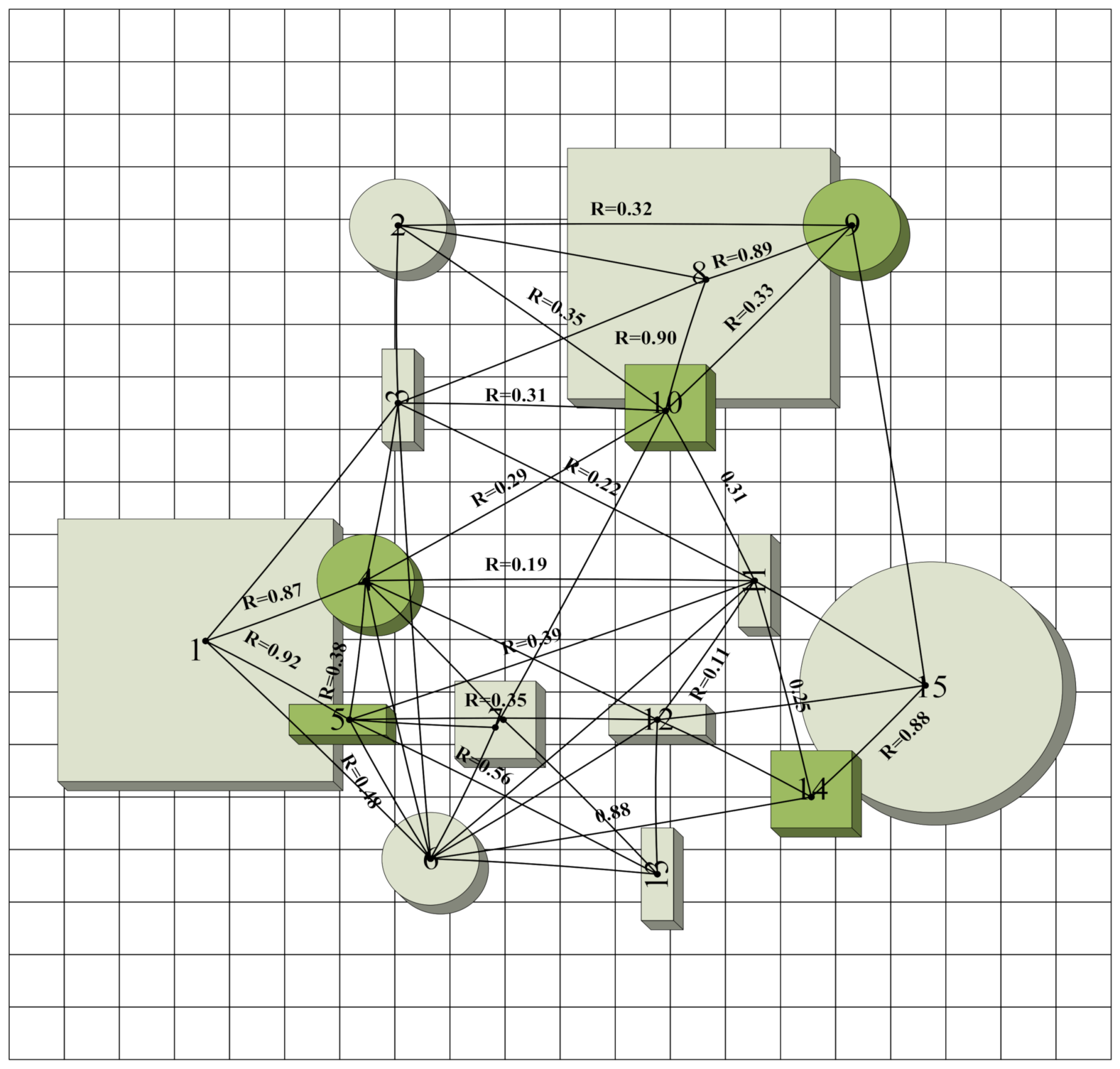
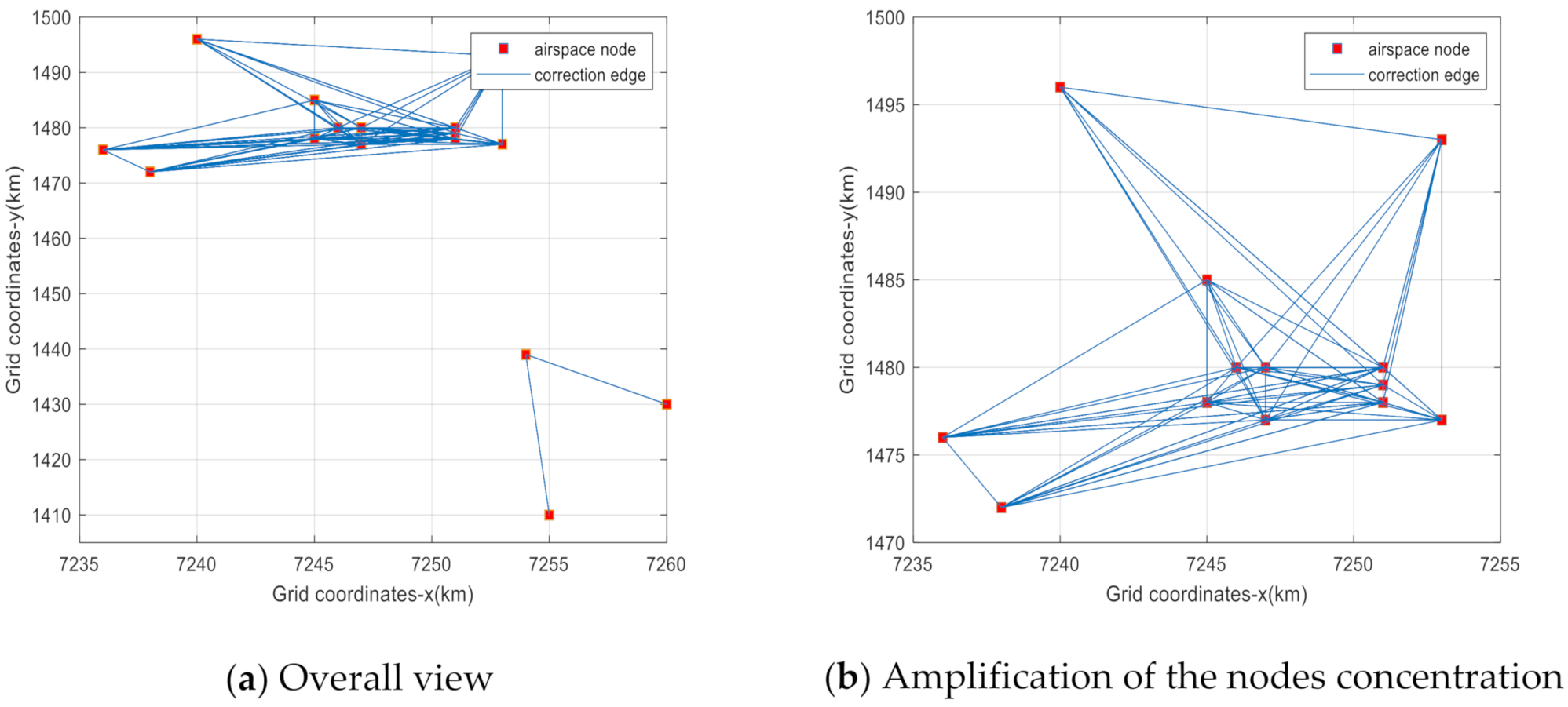
5.2. Construction of Airspace Association Network

In this part, the airspace correlation network model in Guangzhou area is established by calculating the airspace correlation degree (as shown in Figure 5a), and the concentrated area is enlarged to obtain Figure 5b.

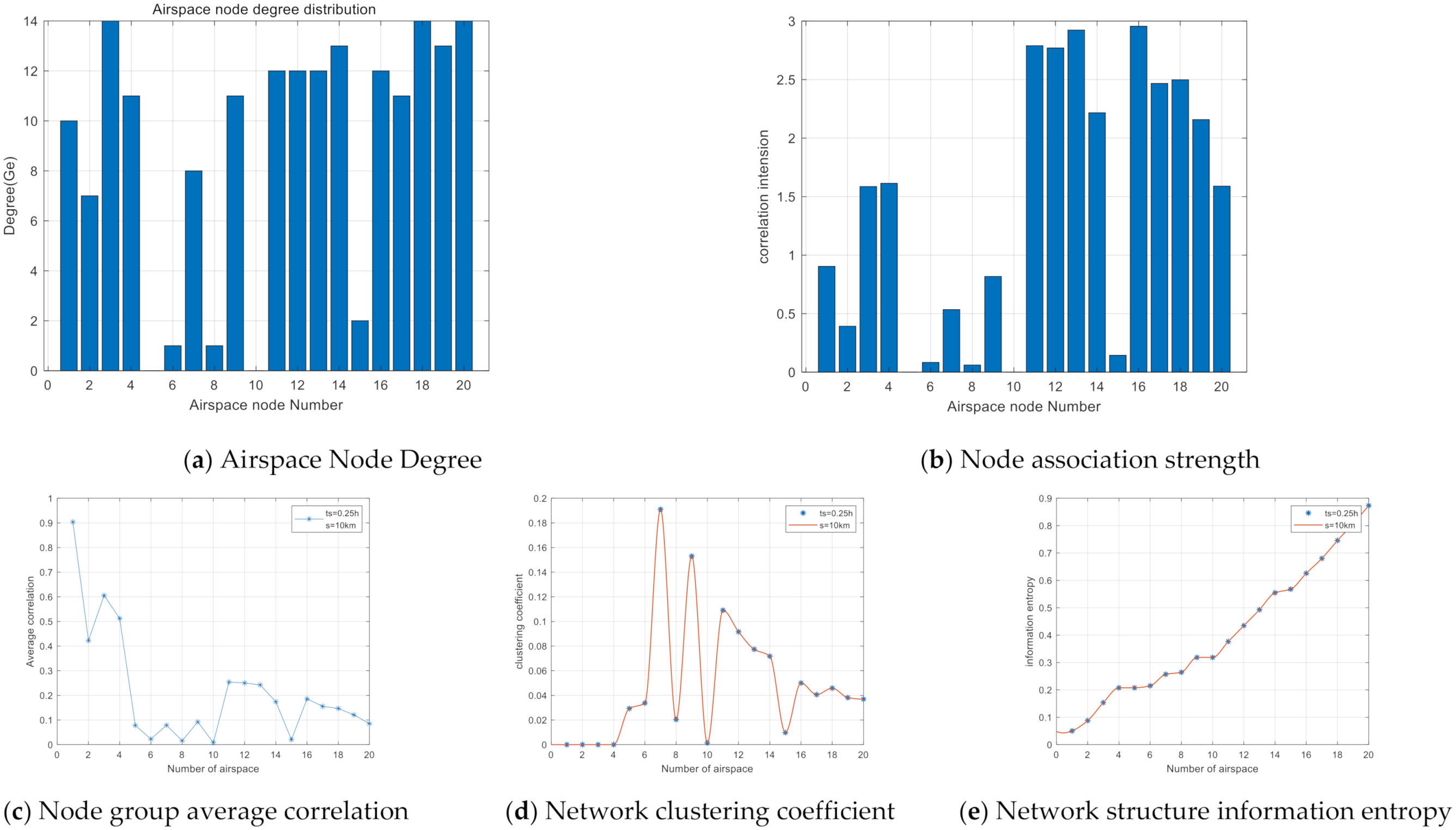
5.3. Analysis of Network Topology Characteristics

In order to deeply analyze the network structure and relationship, the airspace network in Guangzhou area is quantitatively analyzed by using the network topology feature index defined in Section 4.2. Through calculation and simulation, the airspace network in Guangzhou area includes 20 airspace nodes and 76 nodes are connected to each other. The specific parameters are as shown in

Table 8. Network Specifications.

Feature Index	Max	Min	Average
Airspace Node Degree	14	0	8.9
Node association strength	3.299	0	1.453
Node group average correlation	0.855	0.011	0.208
Network clustering coefficient	1.018	0	0.101
Network structure information entropy	3.986	0.233	1.900

.

It can be found from the table that each airspace node is connected to 8.9 airspace nodes on average, and the average correlation degree with other nodes in the network is 1.453, which is a high degree of correlation; the average node information degree is only 0.05 and the network aggregation coefficient is only 0.101 It shows that there are sparse and loose areas in the network, some airspace nodes are far away from the central area of the network, and the degree of correlation is small; the information entropy of the network structure is 3.986, which indicates that the order of the overall network is general, and there is the possibility of fluctuations. Using program simulation, a number of network topology characteristics are obtained as Figure 6a–e.

From the data, it can be found that airspace No. 3, No. 18, and No. 20 have the largest airspace node degree and node information degree, and the No. 11 airspace has the highest association strength of airspace nodes. Based on the above data analysis and statistical laws, it is found that the node correlation degree and network clustering coefficient of the airspace network in Guangzhou are relatively large, but the average correlation is not high, basically conforming to the characteristics of the small-world network. It also increases accordingly, indicating that the more airspace nodes, the stronger the complementarity between the nodes, the higher the stability of the entire airspace network, and the more orderly distribution.

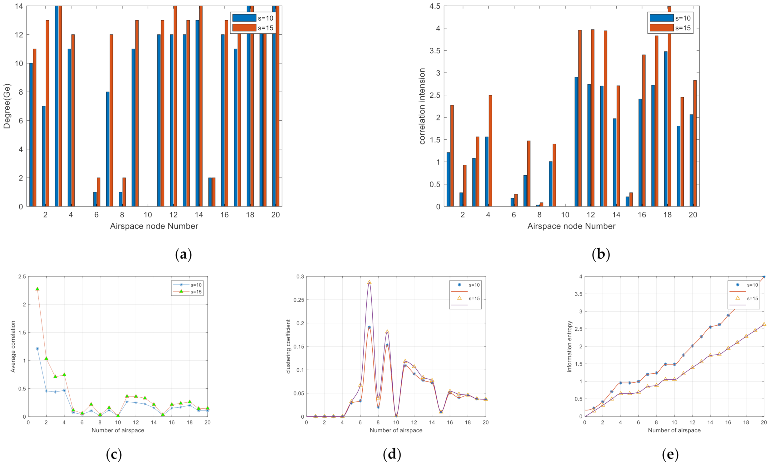
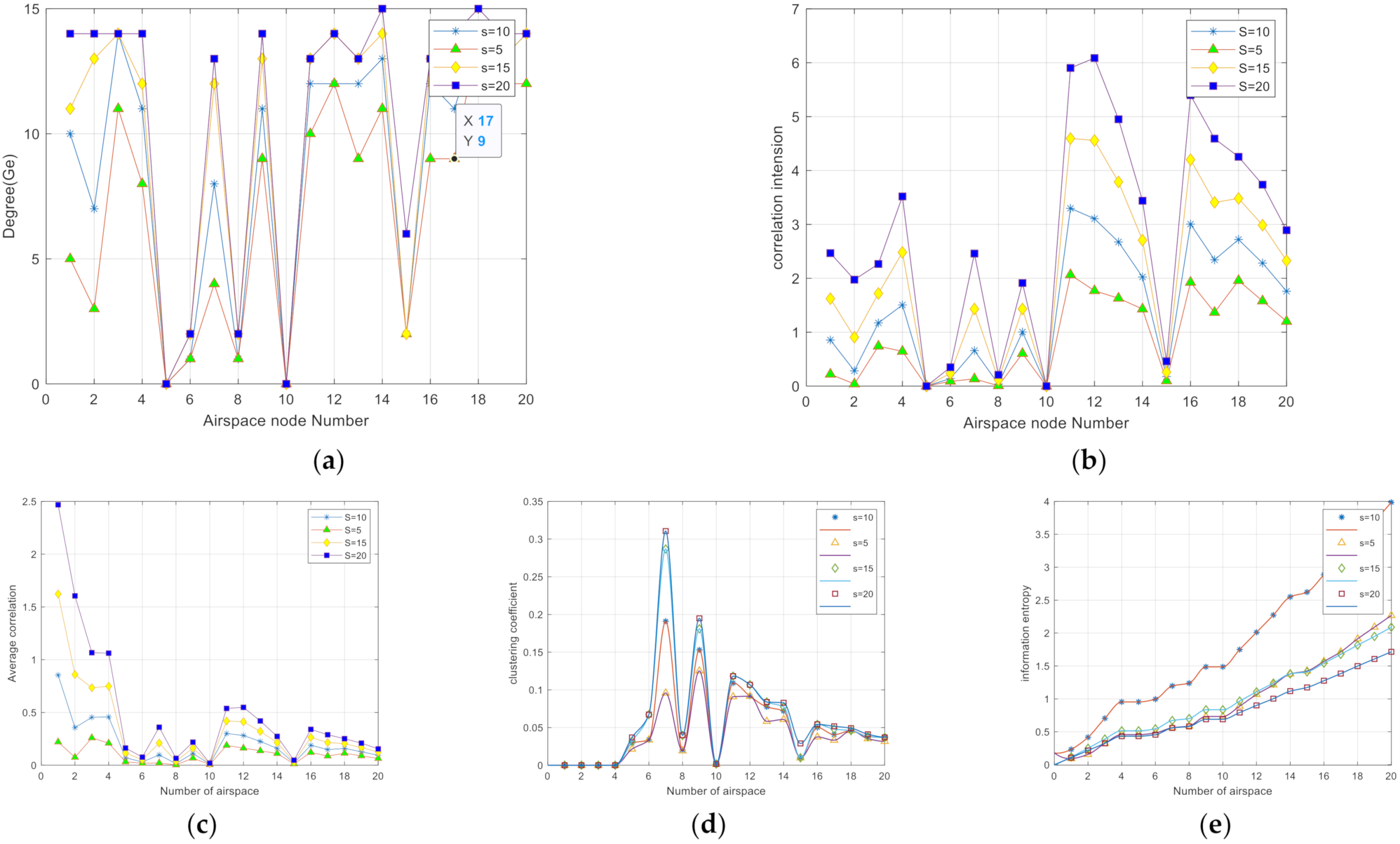
5.4. Multiple Simulation Analysis

Through an analysis of the theoretical derivation part, it is found that the attribute parameters of the airspace correlation network model are mainly affected by the specific correlation degree value between airspace, and there are two factors that have a great influence on the correlation degree value. One is the safety margin between airspace. degree time, and the other is the safety distance between airspace. When using the Analytic Hierarchy Process to calculate basic symmetric operator weights, according to empirical analysis, the importance of the safety distance between airspace is set to be much greater than the safety margin time between airspace. In order to further test and determine the importance of these two factors, several groups of experimental simulations were carried out by controlling a single variable. The specific simulation results are as follows:

Simulation 1: What is considered here is that the airspace use unit has higher requirements on the time accuracy, the purpose is to avoid electromagnetic interference caused by other airspace use tasks and thus affect the normal implementation of airspace tasks. Assuming that the safety margin time is placed at the highest priority, the safety distance between airspace is kept unchanged, the safety margin time between airspace is doubled to 0.5 h, and other experimental conditions remain unchanged. From the experimental results, the node degree and aggregation coefficient in the airspace correlation network before and after adjustment have not changed the remaining three parameters. The changes are compared in the following Figure 7.

The simulation comparison results of simulation 1, on the whole, show that the inter-space safety margin time has little influence on the inherent airspace association network. From the fact that the airspace node degree and node association strength in the network have not changed, it can be inferred that for the entire airspace association network the structure has not changed; that is, the existing conflicting airspace has not been added or reduced in the entire network. The influence of the safety margin time between airspace mainly lies in the degree of association of the nodes in the airspace between the networks. The increase in the safety margin time may lead to greater temporal association with the originally associated airspace, resulting in a larger comprehensive association. Figure 7a,b in Simulation 1 show that the association strength and average association degree of the airspace association network increase to different degrees with the increase in the safety margin time between airspace. At the same time, as the safety margin time increases, the spatial association network increases the amount of information due to the increase in the degree of association between some nodes, resulting in a decrease in the order of the entire network.

Simulation 2: It is considered here that some air activities require a large airspace range and sufficient airspace safety distance to ensure the safe and smooth implementation of air tasks, such as some aerospace exhibitions and performances. Assuming that the airspace safety distance is the highest priority, the safety margin time between airspace is kept unchanged, the safety distance between airspace is adjusted to 15 km, and other experimental conditions remain unchanged. From the experimental results, the characteristic parameters of the airspace correlation network have changed significantly before and after the adjustment. The specific changes are compared in Figure 8.

Compared with the results of simulation 1, the simulation comparison of simulation 2 clearly shows that the safety distance between airspace has caused structural changes and reorganizations to the entire airspace association network. From the comparison (a) and (b) of simulation 2, it can be seen that the node degree and node association strength of the network have changed, indicating that the airspace with association (conflict) relationship has been added or reduced in the network, and this is also an airspace association network. The most important parameter index is to keep the safety margin time unchanged. The change in the safety distance affects the structure of the entire network, including the aggregation coefficient of network nodes and other factors, which verifies the importance of the above for the safety distance between airspace as the highest assumption.

Simulation 3: From the results of simulation 1 and 2, it is inferred that the safety distance between airspace has a greater impact on the entire airspace association network. However, in simulation 2, the safety distance between airspace is only changed once, resulting in fewer experimental samples that can be studied. Considering that in the process of actual airspace use, the requirements of airspace use units are often more diverse and different, so in Experiment 3, more representative variable values with greater differences were selected for experimental simulation. The experimental comparison is shown in Figure 9.

The experimental results of simulation 3 further verify that the safety distance between airspace has the greatest impact on the airspace correlation. With the change in safety distance, not only the association of the entire airspace association network has changed, but also the degree of association between nodes has also changed, indicating that the influence factor of safety distance between airspace has multiple and complex effects on the association relationship between airspace. Therefore, in the current work of resolving airspace conflicts, the conflict between airspace is resolved mainly by adjusting the usage time of the two pieces of airspace so that there is no conflict in the time dimension. However, this digestion method is only suitable for the case where the mission airspace is small, and the flight mission is not busy. If considering the rapid increase in air demand in the future and the rapid increase in the number of mission airspace, the limitation of the method of adjusting airtime is more obvious and the tactical role and purpose of the mission airspace are easily destroyed. Therefore, in the future, it will still be necessary to explore new ideas for airspace conflict resolution that can highly match the mission requirements in the spatial dimension.

6. Conclusions

This paper proposes an airspace network modeling method based on complex network theory. While making reasonable assumptions about the network topology model, five network feature indices are defined to help analyze network characteristics. Based on this, 20 airspace nodes were collected in Guangzhou and surrounding areas to establish the airspace network structure in Guangzhou, and statistical analysis was carried out according to the index parameters of performance characteristics. It reflects the degree of association and relative relationship between airspace, basically achieving the purpose of establishing an airspace network using complex network theory and providing a model basis for further research, such as subsequent research on airspace clustering. The main conclusions are as follows:

(1)

For the first time, the establishment of an airspace association network is proposed based on the relationship between airspace, which can assist airspace managers in decision making with an intuitive and clear network map. Especially in the airspace conflict resolution task, the task object has changed from all airspace to the airspace within the network, excluding the airspace that has no relationship outside the network, which greatly improves work efficiency and accuracy. This also lays the foundation for future large-scale airspace conflict detection and resolution.

(2)

The airspace association network model established based on the association symmetric operator can intuitively and clearly represent the association relationship of airspace nodes and provide certain decision making assistance for the deployment of air missions and the arrangement of related air activities.

(3)

The safety margin time and safety distance between airspace are the two most important factors in determining the relationship between airspace. These two factors should be comprehensively considered when planning airspace to ensure airspace operations are smoother and more ordered.

(4)

The impact of the safety distance between airspace on the entire airspace network is multiple and complex, and it is easy to adjust the safety distance between airspace and thus cause other conflicts in chains. However, adjusting the safety distance between airspace is an important direction for resolving airspace conflicts in the case of large-scale mission airspace in the future. It is worth exploring and researching in depth.

(5)

The construction of the airspace correlation network proposed in this paper also has some shortcomings. The main disadvantage is that the network construction is relatively complicated and the preparation work in advance, such as solving the basic symmetric operator, is cumbersome, and the correlation degree is closely related to the basic symmetric operator. If there is a calculation error in the early stage, then the final airspace association network will also have a series of errors, and these are not easy to find and correct.

References

1. Srivastava, A.; St Clair, T.; Pan, G. On-demand assessment of air traffic impact of blocking airspace. Aeronaut. J. 2018, 122, 1985–2009. [Google Scholar] [CrossRef]
2. Zhang, W.; Jiang, H. The concept of airspace. J. Beijing Univ. Aeronaut. Astronaut. Soc. Sci. Ed. 2021, 34, 127–133. [Google Scholar]
3. Bauranov, A.; Rakas, J. Designing airspace for urban air mobility: A review of concepts and approaches. Prog. Aerosp. Sci. 2021, 125, 100726. [Google Scholar] [CrossRef]
4. Rosenow, J.; Chen, G.; Fricke, H.; Sun, X.; Wang, Y. Impact of Chinese and European Airspace Constraints on Trajectory Optimization. Aerospace 2021, 8, 338. [Google Scholar] [CrossRef]
5. Jing, M. Design of general aviation airspace planning and management system based on Google Earth. J. Phys. Conf. Ser. 2021, 1786, 012032. [Google Scholar]
6. Oktal, H.; Yaman, K.; Kasimbeyli, R. A Mathematical Programming Approach to Optimum Airspace Sectorisation Problem. J. Navig. 2020, 73, 599–612. [Google Scholar] [CrossRef]
7. Zhang, K.; Liu, Y.; Wang, J.; Song, H.; Liu, D. Tree-Based Airspace Capacity Estimation. In Proceedings of the Integrated Communications Navigation and Surveillance Conference (ICNS), Herndon, VA, USA, 8–10 September 2020. [Google Scholar]
8. Rezo, Z.; Steiner, S.; Mihetec, T. European Airspace (DE)Fragmentation Assessment Model. Promet-Traffic Transp. 2021, 33, 309–318. [Google Scholar] [CrossRef]
9. Baspnar, B.; Balakrishnan, H.; Koyuncu, E. Optimization-Based Autonomous Air Traffic Control for Airspace Capacity Improvement. IEEE Trans. Aerosp. Electron. Syst. 2020, 56, 4814–4830. [Google Scholar] [CrossRef]
10. Zhang, J.; Xu, X.; Ning, X. Network-based airspace model. J. China Civ. Aviat. Acad. 2002, 20, 1–5. [Google Scholar]
11. Gurtner, G.; Vitali, S.; Cipolla, M.; Lillo, F.; Mantegna, R.N.; Micciche, S.; Pozzi, S. Multi-scale analysis of the European airspace using network community detection. PLoS ONE 2014, 9, e94414. [Google Scholar] [CrossRef] [Green Version]
12. Wang, X.; Gao, J.; Zhao, M. Analysis of complex network characteristics and invulnerability of control sectors. Inf. Secur. Res. 2018, 4, 157–162. [Google Scholar] [CrossRef]
13. Gao, J. Airspace Sector Network Analysis and Survivability Research Based on Complex Network; Civil Aviation University of China: Tianjin, China, 2018. [Google Scholar]
14. Qi, Y.; Gao, J. Airspace sector network cascade failure resilience and optimization strategy. J. Aeronaut. Astronaut. 2018, 39, 356–364. [Google Scholar]
15. Wang, X.; Gao, J.; Zhao, M. Modeling and characteristic analysis of complex network of air traffic control sectors. J. Civ. Aviat. Univ. China 2019, 37, 7–11. [Google Scholar]
16. Wang, X.; Miao, S. Structural characteristic analysis and resilience assessment of airspace sector network. J. Beijing Univ. Aeronaut. Astronaut. 2021, 47, 904–911. [Google Scholar]
17. Chen, N.; Kong, J. Analysis of airspace sector network characteristics and invulnerability based on complex network theory. Sci. Technol. Innov. 2021, 2021, 110–111. [Google Scholar]
18. Vargas, L.G. An overview of the analytic hierarchy process and its applications. Eur. J. Oper. Res. 1990, 48, 2–8. [Google Scholar] [CrossRef]
19. Ringnér, M. What is principal component analysis? Nat. Biotechnol. 2008, 26, 303–304. [Google Scholar] [CrossRef]
20. Rao, C.R. The use and interpretation of principal component analysis in applied research. Sankhyā Indian J. Stat. Ser. A 1964, 26, 329–358. [Google Scholar]
21. Zhu, Y.; Tian, D.; Yan, F. Effectiveness of entropy weight method in decision-making. Math. Probl. Eng. 2020, 2020, 3564835. [Google Scholar] [CrossRef]
22. Zhou, R.; Ren, H. A review for topology identification of complex networks. J. Xi’an Univ. Technol. 2017, 33, 80–85. [Google Scholar]
23. Cao, L.; Huang, G. Concept design and construction algorithm of rough complex networks. J. Intell. Fuzzy Syst. 2017, 33, 1441–1451. [Google Scholar] [CrossRef]
24. Pluhacek, M.; Senkerik, R.; Viktorin, A.; Zelinka, I. Creating Complex Networks Using Multi-Swarm PSO. In Proceedings of the 8th International Conference on Intelligent Networking and Collaborative Systems (INCoS), Ostrava, Czech Republic, 7–9 September 2016. [Google Scholar]
25. Tian, R.; Zhang, Y. Research on target node analysis technology in complex network. J. Discret. Math. Sci. Cryptogr. 2018, 21, 1157–1165. [Google Scholar] [CrossRef]
26. Wu, Y.; Chen, Z.; Yao, K.; Zhao, X.; Chen, Y. On the Correlation between Fractal Dimension and Robustness of Complex Networks. Fractals-Complex Geom. Patterns Scaling Nat. Soc. 2019, 27, 1950067. [Google Scholar] [CrossRef]
27. Wen, T.; Jiang, W. An information dimension of weighted complex networks. Phys. A Stat. Mech. Appl. 2018, 501, 388–399. [Google Scholar] [CrossRef]
28. Zhang, H.; Hu, C.; Wang, X. Brittleness analysis and important nodes discovery in large time-evolving complex networks. J. Shanghai Jiaotong Univ. Sci. 2017, 22, 50–54. [Google Scholar] [CrossRef]
29. Lv, L.; Wu, J.; Lv, H. A Community Discovery Algorithm for Complex Networks. J. Phys. Conf. Ser. 2020, 1533, 032076. [Google Scholar] [CrossRef]
30. Dai, J.; Huang, K.; Liu, Y.; Yang, C.; Wang, Z. Global Reconstruction of Complex Network Topology via Structured Compressive Sensing. IEEE Syst. J. 2021, 15, 1959–1969. [Google Scholar] [CrossRef]
31. Yang, X.; Wen, S.; Liu, Z.; Li, C.; Huang, C. Dynamic Properties of Foreign Exchange Complex Network. Mathematics 2019, 7, 832. [Google Scholar] [CrossRef] [Green Version]
32. Watts, D.J.; Strogatz, S.H. Collective dynamics of ‘small-world’ networks. Nature 1998, 393, 440–442. [Google Scholar] [CrossRef]
33. Faloutsos, M.; Faloutsos, P.; Faloutsos, C. On power-law relationships of the internet topology. ACM SIGCOMM Comput. Commun. Rev. 1999, 29, 251–262. [Google Scholar] [CrossRef]
34. Dudziak-Gajowiak, D.; Juszczyszyn, K. Complex Networks Modelling of Supply Chains in Construction and Logistics. In Proceedings of the International Conference on Numerical Analysis and Applied Mathematics (ICNAAM), Rhodes, Greece, 13–18 September 2019. [Google Scholar]
35. Xu, Y.; Cheng, L. Review of Logistics Networks Structure Based on Complex Networks. In Proceedings of the 36th Chinese Control Conference (CCC), Dalian, China, 26–28 July 2017. [Google Scholar]
36. Li, M.; Han, J. Complex Network Theory in Urban Traffic Network. In Proceedings of the 2nd International Conference on Materials Science, Machinery and Energy Engineering (MSMEE), Dalian, China, 13–14 May 2017. [Google Scholar]
37. Du, F.; Huang, H.; Zhang, D.; Zhang, F. Analysis of characteristics of complex network and robustness in Shanghai metro network. Eng. J. Wuhan Univ. 2016, 49, 701–707. [Google Scholar]
38. Zhang, X.; Chen, B. Study on node importance evaluation of the high-speed passenger traffic complex network based on the Structural Hole Theory. Open Phys. 2017, 15, 1–11. [Google Scholar] [CrossRef]
39. Zhigang, Z. Research on Invulnerability of Wireless Sensor Networks Based on Complex Network Topology Structure. Int. J. Online Eng. 2017, 13, 100–112. [Google Scholar]
40. Xu, N.-R.; Liu, J.-B.; Li, D.-X.; Wang, J. Research on Evolutionary Mechanism of Agile Supply Chain Network via Complex Network Theory. Math. Probl. Eng. 2016, 2016, 4346580. [Google Scholar] [CrossRef] [Green Version]
41. Yali, Z.; Lifu, W.; Zhi, K.; Liqian, W. Quantitatively computational controllability of complex networks. In Proceedings of the 2018 Chinese Control and Decision Conference, Shenyang, China, 9–11 June 2018. [Google Scholar]
42. Li, K.; Sun, Q. Research progress of complex network synchronization control. In Proceedings of the International Conference on Intelligent Design (ICID), Xian, China, 11–13 December 2020. [Google Scholar]
43. Chakraborty, A.; Vineeth, B.S.; Manoj, B.S. On the Evolution of Finite-Sized Complex Networks with Constrained Link Addition. In Proceedings of the 2018 IEEE International Conference on Advanced Networks and Telecommunications Systems, Indore, India, 16–19 December 2018. [Google Scholar]
44. Garlaschelli, D.; Ruzzenenti, F.; Basosi, R. Complex Networks and Symmetry I: A Review. Symmetry 2010, 2, 1683–1709. [Google Scholar] [CrossRef] [Green Version]
45. Chen, Y.; Zhao, Y.; Han, X. Characterization of Symmetry of Complex Networks. Symmetry 2019, 11, 692. [Google Scholar] [CrossRef] [Green Version]
46. Sloboda, F. A parallel projection method for linear algebraic systems. Apl. Mat. 1978, 23, 185–198. [Google Scholar] [CrossRef]
47. Hu, J.; Xiao, J.; Chen, Z. Solving the Parallel Projection Graph of Space Plane Figures. Comput. Mod. 2001, 72, 99–102. [Google Scholar]
48. Wang, Z.; Shi, M.; Li, Z.; He, A. Three-dimensional flow field reconstruction based on parallel projection method. Acta Opt. Sin. 2002, 22, 556–559. [Google Scholar]
49. Zhang, F.; Qin, Z.; Jing, W. Algorithm Research and Implementation of Parallel Projection of 3D Graphics. J. Univ. Electron. Sci. Technol. China 1994, 23, 510–516. [Google Scholar]
50. ICAO DOC 8168; Procedures for Air Navigation Services: Aircraft Operations. ICAO: Montreal, QC, Canada, 2006.
51. Shan, H.; Cheng, C.; Chen, B. A Geospatial Data Storage Architecture Design Method Based on GeoSOT Grid. J. Surv. Mapp. Sci. Technol. 2018, 35, 311–314, 320. [Google Scholar]
52. Xu, X.; Wan, L.; Chen, P.; Dai, J.; Cai, M. Airspace rasterization representation method based on GeoSOT grid. J. Air Force Eng. Univ. Nat. Sci. Ed. 2021, 22, 15–22. [Google Scholar]
53. Lu, N.; Cheng, C.; Jin, A.; Ma, H. An index and retrieval method of spatial data based on GeoSOT global discrete grid system. In Proceedings of the 2013 IEEE International Geoscience and Remote Sensing Symposium-IGARSS, Melbourne, Australia, 21–26 July 2013. [Google Scholar]
54. Song, D.; Cheng, C.; Pu, G.; An, F.; Luo, X. GeoSOT grid application for global remote sensing data subdivision and organization. Chin. J. Surv. Mapp. 2014, 43, 869. [Google Scholar]
55. Saaty, R.W. The analytic hierarchy process—What it is and how it is used. Math. Model. 1987, 9, 161–176. [Google Scholar] [CrossRef] [Green Version]
56. Kuo, T. An Ordinal Consistency Indicator for Pairwise Comparison Matrix. Symmetry 2021, 13, 2183. [Google Scholar] [CrossRef]
57. Sun, M.; Tian, Y.; Ye, B.; He, X.; Zhang, Y. A Review of Research on Flight Conflict Detection and Relief Methods. Aeronaut. Comput. Technol. 2019, 5, 125–128. [Google Scholar]
58. Saaty, T.L. The Analytic Hierarchy Process; McGraw Hill: New York, NY, USA, 1980. [Google Scholar]
Figure 1. Orthographically projection diagram.
Symmetry 14 00790 g001
Figure 2. Spatial correlation function hierarchy model diagram.
Symmetry 14 00790 g002
Figure 3. Sample graph of airspace association network.
Symmetry 14 00790 g003
Figure 4. Spatial node distribution simulation diagram.
Symmetry 14 00790 g004
Figure 5. Schematic diagram of Guangzhou spatial network.
Symmetry 14 00790 g005
Figure 6. Network topology feature index diagram.
Symmetry 14 00790 g006
Figure 7. Experimental results of simulation 1. (a) Comparison of feature index degree. (b) Comparison of feature index correction. (c) Comparison of feature index average correlation. (d) Comparison of feature index clustering coefficient. (e) Comparison of feature index information entropy.
Symmetry 14 00790 g007
Figure 8. Experimental results of simulation 2. (a) Comparison of feature index degree. (b) Comparison of feature index correction. (c) Comparison of feature index average correlation. (d) Comparison of feature index clustering coefficient. (e) Comparison of feature index information entropy.
Symmetry 14 00790 g008
Figure 9. Experimental results of simulation 3. (a) Comparison of feature index degree. (b) Comparison of feature index correction. (c) Comparison of feature index average correlation. (d) Comparison of feature index clustering coefficient. (e) Comparison of feature index information entropy.
Symmetry 14 00790 g009