Abstract
The present communication revisits the almost century-and-a-half-old problem of some identical small magnets floating freely on the water’s surface under the action of a superimposing magnetic field created by a stronger magnet placed above them. Originally introduced and performed by Alfred Marshall Mayer and reported in a series of articles starting from 1878 onward, the proposed experiments were intended to provide a model (theoretical and educational) for the building block of matter that, at a microscopic level, is the atom. The self-organizing patterns formed by the repelling small magnets under the influence of a single attractive central force are presented in a slightly different reenactment of the original experiments. Although the set-up is characterized by an axially symmetric magnetostatic structure, and the floated magnets are all identical, the resulting equilibrium patterns are not necessarily symmetrical, as one would expect. To the authors’ best knowledge, the present communication proposes for the first time a quantitative approach to that extremely complex conceptual problem by providing a methodology for computing the equilibrium point coordinates in the case of n = 1…20 floating magnets, as proposed by the original A.M. Mayer experiments. A good agreement between the experiments and computed data was demonstrated for n = 2…15 (1st variant), but it was less accurate while still preserving the experimental set-up configurations for n = 15 (2nd variant)…20. Finally, this study draws the conclusions from the performed experiments and their corresponding computer simulations, identifies some open issues, and outlines possible solutions to address them, as well as future developments concerning the subject in general.
1. Introduction
Toward the end of the 19th century, the significant progress made in particle physics paved the way for the adoption of a radically new concept the atom, naturally followed by the molecule, isomerism, allotropy, etc. Its existence, logically necessary in science and more and more conceptually accepted by scientists at the turn of the 20th century, needed a more concrete illustration to be understood for the benefit of all the branches of physics: electromagnetism, thermodynamics, chemistry, later quantic mechanics, etc.
The American physicist and experimentalist Alfred Marshall Mayer was part of the effort devoted to introducing such a novel concept for that time. In a series of articles, the first being published in 1878, he contributed to the basic understanding of the structure of the atom. Mayer devised a series of experiments in which some magnetized identical steel needles run through tiny corks, acting like permanent magnets (PMs), are floated on the water under the attractive force of a stronger oblong cylinder magnet placed above [1,2,3,4,5,6]. The latter has the north pole facing the water surface, thus exerting an attractive force to the south pole of the upward-oriented parallel needles. Being similarly magnetized and parallel, the needles repel themselves, with equilibrium being reached within the system when the attractive and repulsive forces cancel each other out for all the magnets, thus generating various symmetrical or nonsymmetrical equilibrium patterns in the process. Intended to provide a visual illustration of the forces exerted within the atom, the experiment had a variant proposed by Mayer himself, in which the parallel magnets are hanging, attached to silk strings all tied together in a knot. In that case, gravity simply replaces the superimposing magnet, as the mutually repelling PMs are all drawn by the radial component of their weight to the center placed underneath the common suspension point. The experimental set-up is accompanied by an optical device allowing the projection of the resulted equilibrium patterns onto a screen for classroom didactical purposes.
The floating magnets experiment was carried out for a total number up to n = 51 PMs, but Mayer provided actual graphical illustrations for the resulted geometrical equilibrium arrangements up to only n = 20 (except n = 19, a case omitted in all his recurrent articles on the subject) [3,4,5,6]. Interestingly, starting with n = 8, some experiments provided more than one equilibrium configuration, lettered by Mayer as a, b, and c, an order reflecting the increasing instability of the obtained variants. Through exterior mechanical intervention (e.g., vibrations, pushing, or shaking), the equilibrium may become more stable, following the transformation of and, finally, (the more stable variant). Moreover, with the increasing number of PMs, hierarchical self-organization of the PMs could be put in evidence. Mayer termed the concentrical geometrical figure components of the equilibrium patterns as “primary”, “secondary”, “tertiary”, etc. These two aspects allowed an easy-to-understand illustration of the electrons gravitating around the atom’s nucleus distributed on different energy level orbits for the latter, as well as for the concept of isomerism for the former.
In that respect, the first to see real potential following these experiments was the reputed physicist William Thomson (later known as Lord Kelvin), who enthusiastically embraced Mayer’s 2D magnetostatic illustration of the 3D dynamic equilibrium exhibited by electrons orbiting the nucleus (i.e., “kinetic equilibrium of columnar vertices”, as termed by the author) [7]. Several academics followed that path at the beginning of the 20th century, as presented in the comprehensive literature review on the subject, from a historical perspective, published in 1979 by H.A.M. Snelders [8].
The interest sparked by Mayer’s experiments materialized in a couple of new variants of the initial set-up, intending to improve them by eliminating some inherent shortcomings affecting the expected symmetry of the obtained equilibrium configurations. A more flexible variant of the experiment uses, instead of the suspended magnet, a cylinder electromagnet, whereby the DC current carried by the winding allows easy adjustment of the superimposed magnetic field strength.
In 1880, R.B. Warder and W.P. Shipley proposed a significantly different approach to provide a central attractive force, namely by the use of an electric current running through a coil wound around the water-containing vessel [9]. By doing so, the mutually interacting magnetized objects were repelled from the edge of the vessel and toward its center. The authors provided approximate estimation formulas for the interactions involved in achieving the balance of forces without going into any further details concerning the equilibrium patterns’ determination for the system of n magnetized bodies. In fact, equilibrium diagrams were provided for n = 9 and 10, each with two distinct variants. As one would expect, there are significant differences when compared with the corresponding original experiments due to the different natures of the two set-ups.
Next on the timeline, in 1888, James Monkman, encouraged by William Thomson, proposed an electric field variant of the original experiment, in spite of the fact that electrostatic forces are commonly known to be less intense than their magnetic counterparts [10]. Specifically, the magnetized needles were substituted with parallel cylinders and electrified by means of induction when a charged sphere was placed above them, playing the role of the initial attracting magnet. Up to 20 electrified cylinders were used in the experiment, yielding numerous similarities with Mayer’s equilibrium patterns. Nonetheless, some specific patterns had been obtained by Monkman only in the magnetic field created by an electromagnet. In spite of that, the numerous similarities appearing in the two sets of experiments would suggest the virtual “universality” of Mayer’s equilibrium patterns, possibly valid for some other experiments involving mutually repellent objects subjected to an exterior attracting force, regardless of their physical nature.
In an effort to overcome the inherent uneven magnetization achieved for the steel sawing needles, and in the quest to obtain “more” symmetrical equilibrium patterns, R.W. Wood (1898) used small steel spheres (“bicycle balls”) as self-organizing magnetized particles, with the water being replaced by filtered mercury [11]. Although not stated explicitly, the balls were not magnetized prior to the experiment, with that process happening as the floating objects were being submitted to the exterior magnetic field produced by an electromagnet and hence practically simultaneously to the self-organizing process. The resulted equilibrium patterns that were being reported in the paper were considered by the author to be symmetrical up to about 30 particles, albeit in the presented diagrams (20 in total), that characteristic was sometimes rather inconclusive. Certainly, results partially analogous to Mayer’s equilibrium patterns have been obtained in this modified experiment.
A.W. Porter proposed in 1906 a variant of the experiment without making use of the suspended magnet at all [12]. The floating, mutually repelling PMs were held together by superficial tensions in a vessel filled with water to overflowing. The resulting equilibrium patterns differed from those predicted by Mayer’s experiments. By doing so, Porter intended to prove that the different nature of forces governing the interactions within the atom may lead to various structural configurations.
Later, in 1909, Louis Derr revisited Wood’s experiments with the sole difference that the used “bicycle balls” were previously magnetized by putting them into contact with the polar pieces (“the jaws”) of a strong electromagnet [13]. A complete chart comprising 65 equilibrium diagrams was presented in the article for up to n = 52 floating particles, including the multiple resulting variants for a given n. Here too were similarities with the patterns presented by Mayer identifiable in the case of a small number n of floating particles. Similar to Wood’s results, the symmetry exhibited by the equilibrium patterns was still rather difficult to present as evidence, especially for the arrangements formed by larger numbers of floating magnets.
E.R. Lyon reported in 1914 an upscaled version of the Warder and Shipley variant of the experiment, allowing the inclusion of up to 75 magnetized needles [14]. The periodic recurrence of some groups comprising formations of 2…8 members was noticed in the concentric rings around the center, suggesting an interesting correspondence with some chemical elements’ internal structures: O, F, Mg, Al, Si, Cl, etc. An illustration of the concept of “valency” followed naturally, as well as an analogy with the five series of Mendeleev’s periodic table for the “experimental groups” corresponding to the chemical elements.
Following the significant progress in particle physics, the interest shown by the academic community toward the analogy offered by Mayer’s experiments and its variants faded away with time, leaving the self-organization equilibrium pattern determination problem unsolved to the present day. Despite our best efforts, consisting of thorough and careful bibliographical research, only two more recent potentially related articles to Mayer’s experiments can be cited.
A significantly different set-up from the initial experiments, in the absence of a central attracting magnet, was published by D. Pescetti and E. Piano in 1988 [15]. Up to n = 19 identical Alnico magnetic pucks were freely levitated above an air hockey table, being confined inside a Plexiglas ring. The mutually repelling pucks restrained inside a circle provided several symmetrical and nonsymmetrical stable equilibrium configurations. Here too did the symmetry provide more stable variants for a given n, with stability being assessed via the potential energy possessed by the system of PMs. A simple but meaningful illustration was given for n = 5. Without a central attracting magnet present, the pucks would mutually repel one another to the restraining circular wall. Consequently, the particles will lie equally spaced along the periphery (Configuration A: regular pentagon). Next, one particle is pulled to the center, forming Configuration B: a square with a particle in the middle. The latter variant is assessed according to Earnshaw’s theorem, resulting in being stable in the case of tiny displacements inflicted to the puck around the center. Nonetheless, a more ample perturbation will readily transform Configuration B again into A.
The most recent work, dating back to 2004, was published by H.G. Riveros R. et al. [16]. The paper deals with the classical Mayer experiment, though making use of circular permanent magnets instead of magnetized needles. The concentric hierarchical arrangements, in terms of the number of magnets per layer, were described in a tabular manner for n = 1…37 without providing detailed diagrams. The single visual illustration is given in the case of n = 6 variants, namely the centered pentagon and hexagon. Correspondingly, the magnetic potential energy is evaluated for each variant, allowing the authors to conclude that the centered pentagon is more stable than the hexagon. That conclusion would account for the influence of the attracting magnet not present in the Pescetti and Piano experiment, where Configuration B resulted in being less stable than Configuration A (the other way around). Finally, Riveros R. et al. also concluded that the symmetrical equilibrium configurations are more stable than the nonsymmetrical ones in the case of a given n.
Less formally structured material illustrating Mayer’s experiments or their variations can be found on the internet. A useful video presents a reenactment of the classical experiment for n = 15 magnetized needles [17]. In [18], up to n = 20 tiny pill-like Ne-Fe-B magnets were utilized to illustrate the experiment. At some point, two suspending attractive magnets were used to mimic a two-atom molecule having several electrons in common. A possible variation of the classical experiment may consist of replacing the water with pyrolytic graphite, as shown in [19] for n = 5 small PMs. This set-up would eliminate the superficial tensions produced by the liquid, as buoyancy is replaced by the diamagnetic repulsive force exerted by pyrolytic graphite. Thus, only the magnetic forces will come into play, and the resulting equilibrium patterns will be exclusively the result of magnetic forces.
One might possibly wonder whether such an apparently obsolete subject is still relevant in the context of today’s science. As mentioned before, W. Thomson considered the floating magnets analogy with the atom extremely promising, as the system of equal point vortices exhibits dynamic equilibrium arrangements strikingly similar to those obtained in Mayer’s experiments [7,20]. Thus, far from being obsolete, the initial subject may find unexpected connections to more actual ones: the dynamics of point vortices in liquid helium, electron columns in plasma physics, self-assembly of magnetized rotating objects at a liquid–air interface [21,22,23], vortex crystals, vortex lattice theory [24], fluxon behavior in a type II superconductor [25], etc.
In an effort to bridge the gap existing in the literature, the present communication revisits Mayer’s experiments, provides a theoretical foundation for the problem, and presents computation results based on the proposed approach to be further compared with actual experimental results. The remainder of the present communication is structured as follows.
Section 2 describes the materials and methods used to construct the set-up in which the multiple floating magnets experiments are to be reenacted.
Section 3 states the investigated magnetostatics problem and its specific working hypothesis. Next, a theoretical model allowing an analytic approach to the problem is derived, including the parameters necessary to assess the validity and consistency of the obtained results.
Section 4 presents the practical implementation results vs. the experimental data for up to 20 floating magnets.
Section 5 is devoted to a critical discussion and characterization of the obtained results, as well as possible open issues and future research directions on the subject.
Section 6 summarizes the main conclusions of the performed study, putting them into perspective in light of a possible next-level objective, namely stating the morphological laws of self-organizing permanent magnets floating under the action of a central attractive force.
2. Materials and Methods Employed for Reenacting A.M. Mayer’s Multiple Floating Magnets Experiments
Our proposed experiment replicates a slightly different variant of the original set-up initially introduced and reported by Alfred Marshall Mayer, though essentially and conceptually the same [1,2,3,4,5,6]. The needles, magnetized to their remanence and then run through corks in the initial experiment, were substituted in our experiment by Nd-Fe-B small pill-like flat cylinder magnets glued onto transparent plastic circular flat half-shells, acting like small boats. Their north poles faced the water; hence, the south poles were directed upward, facing the air (see Figure 1). Henceforth, the grouping of a PM glued to the plastic shell will be referred to as floating object.
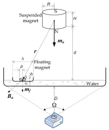
Figure 1.
Depiction of the experimental set-up used to reenact A.M. Mayer’s original experiment, allowing for a convenient method to capture the images of the equilibrium positions formed by the free-floating magnets under the influence of a stronger attracting suspended magnet. A single magnet (n = 1) is represented (all the PMs being identical), aiming to highlight the defining quantitative characteristics of the experiments. Note that the drawing has primarily illustration purposes, and hence the depiction of the experiment is not drawn to scale (e.g., D > d, not the other way around, as represented in the figure to limit the extent of the drawing).
Then, up to n = 20 so prepared identical magnets were floated on shallow water (of 1–1.5 cm in depth) poured onto the bottom of a clear storage box, allowing for easy pattern-forming observation through it. Above the waterline is suspended a significantly stronger Nd-Fe-B vertical downward-magnetized cylinder PM (with the north pole facing the water), similar to the original A.M. Mayer experiment, as shown in Figure 1.
The significance of the quantities shown in Figure 1, used in the sequel, is the following:
- R: suspended cylindrical magnet’s radius;
- H: suspended magnet’s height;
- ρ: floating cylindrical magnets’ radius (identical for n = 1…20);
- h: floating magnets’ height (identical for n = 1…20);
- d: distance from the north pole surface to the waterline;
- D: distance from the camera lens to the bottom of the water tank;
- Δ: diameter of the plastic transparent shells enabling the magnets to float (identical for n = 1…20);
- ma: magnetic moment of the attracting suspended magnet;
- Ba: magnetic flux density produced by the attracting suspended magnet at the center of the floating magnet;
- mf: magnetic moment of the floating magnet;
- r: position vector relative to the center of the suspended magnet;
- Ω: solid angle corresponding to the field of view from the camera lens to the experiment area.
The actual data characterizing the experiments are organized in Table 1.

Table 1.
Data describing the floating magnets experiments.
Additionally, it is worth mentioning that the suspended permanent magnet was of grade N42 (holding approximately 11 kg of load), and the floating identical PMs were of grade N45 (holding approximately 320 g).
Since their south poles faced the air, the mutually repelling floating magnets tended to crowd below the attracting suspended magnet (facing the north pole toward the water surface), forming various symmetrical or nonsymmetrical equilibrium configurations in the process. A photographic image of the proposed set-up, shown in Figure 2, illustrates the experiment carried out in the case a, one of the two symmetrical patterns obtained for n = 20 floating magnets, as we will further present in Section 4. Obviously, exchanging the polarities of all the involved magnets would provide identical experiments from the point of view of the resulting interacting magnetic forces and equilibrium patterns, inclusively. It is important to mention that the optimal distance d was set to 10.5 cm in order to enable up to n = 20 PMs to float (i.e., to avoid the following two limiting cases occurring).
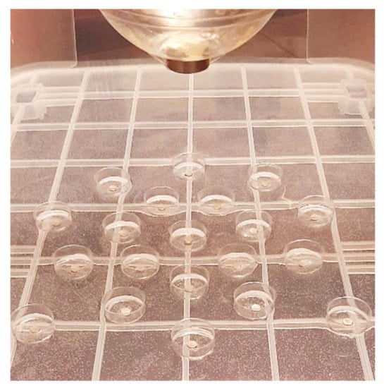
Figure 2.
Photographic image of small identical magnets floating under the action of a stronger suspended magnet in the case na = 20 (subscript a refers to the lowest magnetic potential energy experiment of the two—a and b, as will be further presented in the paper for the 20 floating magnets case). The self-organizing magnets presented a symmetrical equilibrium disposition (along the median longitudinal axis). The pattern diagram is also shown in Figure 5a1.
First, a too narrow separation between the floating magnets is susceptible to inducing the so-called Cheerios effect, which would interfere with the predominantly magnetic forces in the process of generating the equilibrium configurations. At the same time, the floating bodies may come in close contact or even get stuck together in clusters if d becomes too small.
Second, it may happen that the most distant floating magnets (from the central attraction point) become “detached” from a possible equilibrium pattern if d is too large.
Next, the so obtained geometrical figures were recorded by a camera placed underneath the bottom of the tank, allowing an unobstructed view of the self-assembled patterns, contrary to what a view from above would provide due to the presence of the suspended magnet and its fixture. For convenience, to facilitate the experimental determination of the equilibrium point coordinates in the photographic images shot, transparent rulers were glued onto the bottom of the tank along the x- and y-axes. The line of sight of the camera was aligned with the magnetization axis of the suspended magnet (perfectly vertical, ideally). Moreover, to increase the accuracy of the equilibrium points’ determination, the camera was placed sufficiently distant from the bottom of the tank in order to reduce parallax and camera lens image deformation by minimizing the solid angle Ω, as shown in Figure 1.
Additionally, to reduce picture distortion, the water level in the tank was kept as low as possible to ensure the magnets flowed freely but, at the same time, aiming to limit the refraction phenomenon induced by the liquid.
An illustration of a picture shot through the tank’s bottom, allowing us to experimentally determine the equilibrium points’ coordinates, is provided in Figure 3, also in the case of n = 20 (but for a second symmetrical structure, labeled b).
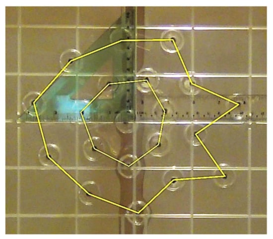
Figure 3.
Photographic image taken through the bottom of the tank in the case nb = 20 (subscript b refers to the second symmetrical configuration obtained for n = 20, possessing a slightly higher magnetic potential energy than that specific to the equilibrium pattern a, shown in Figure 2). Note the two “concentric” polygonal yellow lines forming an outer dodecagon, including a heptagon, and a single magnet in the middle close to the suspended magnet’s axis, passing through the exact center of the image. The pattern is also shown in Figure 5b1.
The authors adopted the same manner proposed by A.M. Mayer in his historic articles to highlight the formed concentric structures by linking the magnets’ equilibrium points with polygonal line segments [4,5,6]. In his proposed analogy with the atom, these concentric polygons would correspond to the different energy level orbits of the electrons attracted by the positively charged nucleus.
Our experiments were carried out successively for n = 1…20 floating magnets, and each equilibrium arrangement was captured in one or several pictures (in the case of 2 or 3 variants), whatever the case may have been. Nonetheless, the trivial case n = 1 was put in place for the purpose of “calibrating” the experiment (i.e., to check whether the suspended magnet was satisfactorily vertically oriented or not). In addition, we checked its alignment with the camera objective and whether the center of the single floating magnet’s equilibrium position coincided with the projection on the water’s surface of the suspended magnet’s axis (the origin of the Cartesian axes of the coordinates, or point O from Figure 4). All these precautions that were taken ensured fairly accurate experimental determinations for the equilibrium points’ coordinates to be further compared with the corresponding computer-simulated results, based on the model proposed in the next section.
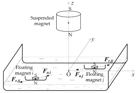
Figure 4.
Magnetic forces exerted in the case of two floating magnets i and j in the xy plane (the water surface).
3. Analytical Model of the Multiple Self-Organizing Floating Magnets Submitted to an Attracting Magnetic Central Force
This section proposes an analytical model for determining the equilibrium position in the case of n = 1…20 floating magnets (up to a number similar to the initial A.M. Mayer experiments [1,2,3,4,5,6]), forming various symmetrical and nonsymmetrical geometric arrangements in the presence of a significantly stronger magnet placed above. The proposed analytical model will allow a numerical approach for solving the resulting 2n nonlinear equilibrium equations, whose solution provides the equilibrium points’ coordinates.
3.1. Context of the Study and Simplifying Hypothesis
Any problem involving the equilibrium position of some permanent magnets must take into consideration a classical result established by Earnshaw’s theorem [26], which prohibits achieving stable equilibrium in a system comprising mutually interacting bodies through forces inversely proportional to the squared distance separating them. Such forces may be of an electrostatic nature or magnetic nature (i.e., between electrically charged bodies or permanent magnets), as was the case for the present problem. After achieving equilibrium, a way to establish whether it was stable or unstable along a certain direction was to estimate the corresponding discriminant of stability for that direction. This approach was considered to check for stability in the case of a single levitated magnet [27,28] or multiple levitated magnets. As a result of how it was defined (see Section 3.3), a negative value of the discriminant of stability was an indicator of unstable equilibrium. To bypass the aforementioned Earnshaw’s theorem consequence, an exterior intervention to the system had to be envisaged: a stabilizing force acting upon the levitated magnet(s) with mechanical contact or by the introduction of a diamagnetic stabilizing body in the proximity of the levitated PM(s), thus not necessitating mechanical contact. At room temperature, the most pronounced diamagnetic behavior is that of pyrolytic graphite, a layered, highly isotropic material exhibiting this property along a perpendicular direction to the deposited layers. In our problem, the stabilizing effect required by Earnshaw’s theorem along the z-axis was simply exerted by buoyancy.
To solve the equilibrium problem for all the simultaneously interacting magnets implies the determination of the magnetic force acting on each of them. That would also imply establishing an analytical formula of the B-field created by a cylinder magnet (necessary in the case of the suspended and the floating magnets alike). Although a closed form has been established for the flux density associated with a cylinder magnet [29], its partial derivatives with respect to the coordinates and further computation necessary for magnetic force evaluation would provide extremely complex relationships and subsequent calculus. Moreover, the latter would be part of a nonlinear system of equilibrium equations to be solved for each degree of freedom (DOF) (in our case, for the x and y coordinates attached to the water surface plane). Solving a system of 2n equations involving such intricate relationships is practically impossible, even for a small number of floating magnets and for the most complex and efficient algorithms running on extremely powerful computing platforms. This highlights the difficulty of the present magnetostatics problem and justifies its scarcity in the scientific literature over the last century and a half and the quasi-absence of any quantitative computation method for determining the PMs’ equilibrium positions (and implicitly, the arrangements they may form to achieve it).
As a result of these considerations, we adopted the following simplifying hypotheses:
Hypothesis 1 (H1).
From a magnetostatics point of view, all the floating and suspended magnets were modeled as magnetic dipoles (in fact, small, magnetized bodies) placed at the center of each cylinder PM. This assumption is pertinent, having in view the net discrepancy existing between R,ρ, and d, as the values shown in Table 1 may suggest. From Figure 2 and Figure 3, one can also notice thatρ was significantly smaller compared with the distance existing between neighboring magnets. As a result of this assumption, the entire magnetic effect of all the PMs was concentrated at the cylinder centers, being accounted for by their magnetic moment vectors mf for the floating magnets and ma for the attracting suspended magnet, as shown in Figure 1.
Hypothesis 2 (H2).
From a mechanics point of view, all the floating bodies were regarded as material points, with their centers of mass coinciding with the magnets’ centers. The superficial tensions at the interface of the floating objects—water were neglected, inferring that they presented a significantly lower magnitude than the magnetic forces involved in the process. Lastly, the Coriolis acceleration associated to the Earth’s rotational movement was neglected in our model.
Hypothesis 3 (H3).
The balance of magnetic forces for achieving equilibrium was solely considered on the xy plane (at the water’s surface), as suggested in Figure 4. Along the z direction, the attractive force exerted by the suspended magnet, the floating object’s force of gravity, its buoyancy, and the water’s surface tension all combined provided a resultant force of zero. Consequently, the system exhibited in our model only two DOFs along the x- and y-axes. Moreover, related to this property, the small submerged part of the floating objects lowered the magnets’ centers practically to the same level as the waterline, as suggested in Figure 1. Consequently, further on in our model, the floating magnets’ centers will be considered as points belonging to the xy plane (z = 0).
Hypothesis 4 (H4).
The magnetic moment mf of the floating magnets was considered to be perfectly vertically oriented (pointing downward). A small PM tends to align itself to the local exterior magnetic field of the flux density (Ba in Figure 1) produced by the suspended magnet, as a compass needle does as the result of terrestrial magnetism. Buoyancy and the quite large diameter of the floating disk bearing the magnet (Δ/2 >ρ) prevented that from happening by maintaining the small magnet axis in a vertical position, as depicted in Figure 1. An eventual significant tilt of the magnet following the orientation of Ba would imply the introduction of a third parameter describing the equilibrium position, apart from coordinates x and y (i.e., the deviation angle with respect to the vertical direction). That would complicate even more the equilibrium equations on the one hand and would represent a deviation from A.M. Mayer’s experiments on the other, since the used magnetized needles were maintained by the buoyancy force provided by the corks in an upright position.
3.2. Magnetic Force Exerted on Mutually Interacting Floating Magnets
As stated in the previous subsection (hypothesis 3), the balance of forces corresponding to the equilibrium state achieved by the floating magnets was considered in the xy plane (the water’s surface). As shown in Figure 4, on every floating magnet, there was an attracting central force directed toward point O, the intersection of the suspended magnet polar axis and the water’s surface (Fa,i, i = 1…n). Consequently, all the floating PMs tended to gather as close as possible exactly underneath the stronger attracting magnet. At the same time, this tendency was limited by the mutual repelling existing between the floating PMs, a fact suggested in Figure 4 by the two antagonist and equal magnitude forces Fr,ij and Fr,ji (Fr,ij = −Fr,ji), where i,j = 1…n and i ≠ j, also belonging to the xy plane. Of course, this type of force appeared between each possible combination of two floating PMs existing at a given time on the water’s surface. Equilibrium was achieved when all the repelling forces between the magnets were balanced by the central attraction force. Let us further denote the total resulting magnetic force acting on the floating PMs in the xy plane as Fi, where i = 1…n.
As mentioned before, by concentrating the entire magnetic effect of the suspended magnet at its center (moment ma), its associated magnetic flux density at a point located by the oriented distance vector r (see Figure 1) is written as [30].
where μ0 is the permeability of free space.
Taking into account that ma is located at point (0, 0, d + H/2), as shown in Figure 1 and Equation (1), we get the z component of Ba in the xy plane in the following form:
where ma = |ma| with ma = −ma k (i.e., opposite to the direction of the z-axis unit vector k).
Similar to Equation (1), a floating magnet j of the magnetic moment mf = −mf k positioned at (xj, yj, 0) on the water surface plane creates at point (x, y, 0) a flux density of the z component having the following expression:
In general, the force exerted on a magnetic dipole (of moment m = −mk), embedded into an external non-homogeneous magnetic field of flux density B, is written as [30]
where i, j, and k are the x-, y-, and z-axes unit vectors, respectively.
In magnetostatics, by virtue of Ampère’s circuital law differential form, we have curl H = J = 0, where H is the magnetic field strength and J is the current density. Hence, we also have curl B = 0, yielding
Consequently, with Equation (5), the force given by Equation (4) may also be written as
Being interested in determining the force exerted on the floating magnets in the xy plane, only the first two components of the force given by Equation (4) will be further considered.
For the floating magnet located at point (xi, yi, 0), the x and y components of the total force acting upon it (due to the suspended magnet and the other remaining n -1 floating PMs) is determined by the use of Equations (2), (3) and (6) combined under the following compact form:
Evidently, a closed form of Equation (7) exists, but its reproduction within the pages of the present paper would amount to an unnecessary extension without adding any significant information to it. Additionally, it must be stressed that special attention should be paid to the actual magnitudes presented in practice by the suspended and floating PMs magnetic moments, namely ma and mf, respectively. In the equilibrium point(s) determination involving permanent magnet problems, the actual magnetization state of the PMs must be thoroughly assessed, since the equilibrium solution is quite sensitive to this aspect. (See in that respect, the levitation problems in [27,28].) It has been experimentally put into evidence that, even in an open-loop configuration, a permanent magnet appears to be less magnetized (less “powerful”) than would be expected by its grade given by its datasheet Br prescribed parameter. That phenomenon occurs even when the magnet is not included in a magnetic circuit to be “powered” by its magnetomotive force (m.m.f.). A self-demagnetization phenomenon occurs even in an open-loop configuration as an edge effect, being dependent on the geometrical shape and size ratios characterizing the magnet in question. A procedure is described in [27,28] to account for the self-demagnetization phenomenon, which is rather feeble but non-negligible in the context of sensitive equilibrium position computation problems. In brief, the permeance coefficient (Pc) formula for a cylinder magnet is calculated as a function of the actual size of the two types of magnets used. Then, the intersection of the second quadrant B-H branch (at 20 °C), belonging to the N42- and N45-grade magnets, with an operating line of slope Pc + 1 provides the actual slightly “demagnetized” flux density magnitudes Bd,a (1.3 T) and Bd,f (1.32 T), respectively. Next, these values are used instead of the remanent flux density (Br) for further evaluation of the magnetic moments, yielding
These corresponding values are listed in Table 1.
3.3. Static Equilibrium of Multiple Floating Magnets
This section is dedicated to the equilibrium equations providing the coordinates for the floating PMs, implicitly constituting the formed self-organizing geometric figures under scrutiny [31,32,33]. A direct consequence of hypothesis 3 of Section 3.1 is that the equilibrium state acquired by the floating PMs can be investigated only in the xy plane. Hence, it suffices to impose zero resultant force acting on each floating PM in the above-mentioned plane. More specifically, this corresponds to solving the following nonlinear system of 2n equations for the unknowns xi and yi (i = 1…n):
In the sequel, (xi, yi) for i = 1…n will represent the solution of Equation (9), namely the equilibrium point’s coordinates for each of the floating PMs. Several parameters will be used as indicators designed to check the consistency of the obtained solution as follows:
- For the discriminants of stability for each floating PM (of index i) at their equilibrium positions [27,28], their role is to test whether or not, at the equilibrium point, a small perturbation (a minute displacement along a given axis) produces restoring forces capable of re-establishing the balance of forces around the respective equilibrium point. Defined as the negative partial derivative with respect to the x, y, and z coordinates at the equilibrium point, we finally obtain the expression of the three axes’ discriminants of stability aswhere Btotal,z,i is the z component of the total flux density in which magnet i is embedded, being created by the suspended magnet and all the remaining (n − 1) floating PMs, and mfz is the z component of the magnetic moment mf = −mf k. Using Equations (2) and (3), we have
- The center of mass corresponding to the PMs at static equilibrium must be in line with the suspended magnet polar axis (point O, the origin of the Cartesian system of coordinates). All the floating bodies (the plastic shells having on top the small magnets) have the same mass. Hence, the system’s center of mass coordinates can be expressed by the following arithmetic means [31]:
- The Hessian matrix of the total magnetic potential energy function Utotal of the system is constructed for assessing whether the static equilibrium points (xi, yi), where i = 1…n, corresponding indeed to local a minimum of Utotal [34]. As in any stable equilibrium problem, the potential energy exhibits at least a local minimum if not a global minimum. Having in view that the equilibrium solution is not unique for several n values, as we will further show in the next section, we will check that the numerically obtained solution of the system in Equation (9) presents at least one local minimum of Utotal. Taking into account that mf = −mf k, and with Equation (11), let us define the total magnetic potential energy as the sum of the same quantity corresponding to each floating PM expressed by the following negative dot product [30]:The Hessian matrix corresponding to , considered a two-variable function of equilibrium points coordinates (xi, yi), is written as [34]where
4. Computer Simulation Results vs. Experimental Determinations
Based on the theoretical approach detailed in Section 3, a computer numerical simulation program was generated in a general-purpose mathematics environment. Basically, it implemented the formulas presented in the previous section, including methods 1–3, which were used for proving the consistency of the obtained result, even though they are somewhat redundant. Nonetheless, they contributed to solidifying the belief that the presented method was trustful, although future improvements or refinements may, of course, be envisaged. The model does not take into account terrestrial magnetism, being considered too weak compared with those of the PMs.
In more detail, the powerful Maple© environment implementation [35] basically consisted of the following steps:
- Input of simulation data: n, the number of floating magnets, the floating magnets’ radius, height, and remanence (demagnetization in an open loop is taken into consideration), the attracting magnet’s radius, height, and remanence (demagnetization in an open loop taken into consideration), and the distance from the attracting magnet’s north pole to the waterline’s surface.
- Analytical implementation of the z component of the flux density formula in Equation (2) for the attracting magnet;
- Analytical implementation of the z component of the flux density formula in Equation (3) for each of the floating magnets due to the proximal presence of the remaining n − 1 ones;
- Analytical implementation of the z component of the total flux density formula in Equation (11) for each of the floating magnets;
- Numerical solving of the system of nonlinear equilibrium equations (Equation (9)), using the “fsolve” routine. Initial arbitrary guess values were used to model the random positioning of the floating magnets at the beginning of the physical experiments. The resulting equilibrium points’ coordinates provided the simulated patterns shown in detail in Figure 5;
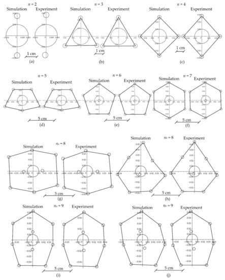
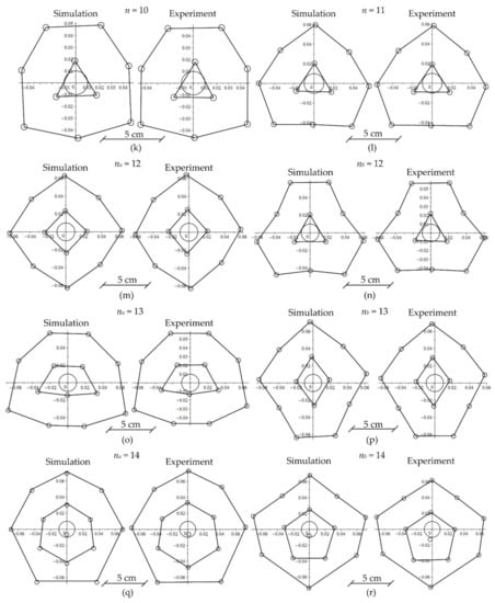
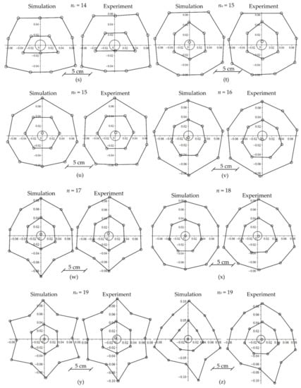
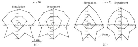 Figure 5. Self-organization equilibrium patterns (simulated vs. experimental) for identical repelling magnets submitted to a central attracting magnetic force in the case of (a) n = 2, (b) n = 3, (c) n = 4, (d) n = 5, (e) n = 6, (f) n = 7, (g) na = 8, (h) nb = 8, (i) na = 9, (j) nb = 9, (k) n = 10, (l) n = 11, (m) na = 12, (n) nb = 12, (o) na = 13, (p) nb = 13, (q) na = 14, (r) nb = 14, (s) nc = 14, (t) na = 15, (u) nb = 15, (v) n = 16, (w) n = 17, (x) n = 18, (y) na = 19, (z) nb = 19, (a1) na = 20, and (b1) nb = 20. The floating magnets are represented by the smaller-radius circles, whereas the suspended stronger magnet is represented by the greater-radius circle, placed at the center of the Cartesian frame of reference.
 - Numerical evaluation of the following quantities: the discriminants of stability (Equation (10)), coordinates of the center of mass corresponding to the system of floating magnets (Equation (12)), total magnetic potential (Equation (13)), and the Hessian matrix (Equations (14) and (15)).
Obviously, the comparison with the measured experimental results provided the ultimate validation for the overall proposed theoretical approach and simulation methodology. The program was run for n = 1…20 floating magnets, having as a primary goal to demonstrate through simulation the same static equilibrium patterns obtained in the experiments the numerical results were being compared with. The core of the generated software was the numerical solving of the 2n nonlinear system of equations of 2n unknowns. The complexity of the numerical procedure heavily depended on the number of unknowns, ultimately imposed by the number n of floating magnets. With an increasing n value, the solution representing the equilibrium coordinates in the xy plane was increasingly dependent on the initial guess values considered in the solving procedure for the nonlinear system of equations. Obtaining a numerical solution that corresponded to a certain experiment implied a succession of trial-and-error runs of the solving procedure starting from different initial guess value (position) sets. Some experiments provided two or three variants for the same number n of floating magnets, corresponding to different levels of local minima for the magnetic potential energy given by Equation (13). The same phenomenon, given as evidence by Mayer himself, made him determined to adopt a specific notation for the variants obtained for a certain value n, as a function of the degree of stability that was acquired in the respective equilibrium configuration. Letter a represented the more stable variants, followed by letters b and c for the less stable variants. The latter can be transformed into a variant a through mechanically induced small perturbations (e.g., vibration, shaking, or moving air). The same notation convention was used by us in labeling the experimental variants we demonstrated (a, b, and even c) in the case of n = 14, as a function of the actual magnetic potential energy level. The lowest one was a (interpreted as the more stable variant), followed by b and c (i.e., an order imposed by an increasing , given by Equation (13)).
The simulation results for n = 2…20 floating magnets with the corresponding experimental results are shown side-by-side as a chart in Figure 5. Note that the experimental results were carefully recorded by photographic means in a manner suggested in Figure 3. For convenience, both the computed and experimental configurations shown in Figure 3 present a depiction of the suspended attracting magnet contour, a circle centered at the origin of the Cartesian axes.
5. Discussion
The present communication’s proposed approach is the culmination of several attempts to identify a viable method for solving the multiple floating magnets equilibrium problem. A thorough review of the literature spanning from the historic works of A.M. Mayer to the present day’s works did not produce any clear indication of how it may be treated beyond the abundant descriptive interpretations. Initially, we identified the two seemingly important and apparently promising investigation directions, which are summarized below.
First, the multiple floating PMs setting has been regarded as an optimization problem. Particle swarm optimization (PSO) was the algorithm of choice, and the objective function to be minimized (to zero) was the sum of the magnitudes exhibited by the net magnetic force acting on each magnet in the xy plane. Several particle population dimensions and particle velocities have been simulated, as well as numerous combinations: small populations and high-velocity particles, the opposite, and something in between. Unfortunately, the results were inconclusive, even for a small number of floating magnets. Apparently, minimizing a sum of strictly positive values to exactly zero (in fact, below a sufficiently small threshold from a numerical point of view) is simply not specific to PSO and thus virtually impossible.
The second approach we tried was based on the minimization of the magnetic potential energy within a 2D, rectangular, sufficiently large search space. The justification of such an approach relies on the natural tendency of a system to settle in a local minimum or absolute minimum energy configurations. The multiple variable minimization algorithm provided implausible solutions, with the PMs being pushed as far away from the central attraction point as the search space permitted (i.e., toward its boundary). Of course, in such a configuration, a minimum magnetic potential energy does not also imply equilibrium.
As proven by the performed experiments, the solution for a certain value n is not unique. The bigger the number n of floated magnets, the greater the variants of possible potential energy local minima expected to be found when equilibrium occurs. Therefore, the problem of determining the equilibrium of n floating magnets inherently presents a degree of randomness concerning how the floating magnets initially positioned at the beginning of the transient phenomenon lead to equilibrium. As a result, this characteristic must be incorporated into the method or algorithm used for equilibrium position determination.
A third possible approach, which we have not explored yet, might be formulated in terms of distance, being a projection of the two opposing forces in balance for each floating PM: the attractive force exerted by the powerful suspended magnet and the combined repulsion forces exerted by the rest of the floating PMs. This may be translated in terms of distance, assuming that each PM tends to minimize its distance to the suspended magnet while maximizing the distance with respect to the rest of the (n − 1) PMs.
The present paper approach relies on the deterministic solving of the nonlinear system of 2n equilibrium equations, having various initial guess values to mimic the randomness of the phenomenon we mentioned earlier. By trial and error, we succeeded with a fairly accurate retrieval of the experimental results for n = 1…15 (variant a), as shown in Figure 5a…t. Furthermore, starting with n = 15 (variant b)…20 from Figure 5u…b1, the results were less accurate in terms of the equilibrium position coordinates but still preserved the shape and concentric polygonal structure given by the corresponding experiments (the number of PMs component of each concentric polygonal ring and their general disposition). The aforementioned deviation from the experimental results might account for several root causes.
First, for an increasing n value, the per-unit floating magnet force provided by the suspended magnet decreased, becoming comparable with the superficial tensions’ magnitudes acting on the floating object. Thus, the superficial tensions (initially ignored by virtue of hypothesis 2 in Section 3.1) may have come into play more significantly, modifying the balance of forces and hence the equilibrium point position. This phenomenon was even more visible for the more distant PMs from the suspended magnet’s axis, since the attractive forces provided by the latter sensibly decreased with distance.
Secondly, also for a larger number of PMs, the more distant magnets had an increased tendency to align their magnetic moment mf along with the local Ba vector orientation, thus deviating more from the assumed perfectly vertical position (hypothesis 4 in Section 3.1), as depicted in Figure 1. A tilted mf would generate a tangential (parallel to the water) component susceptible to modifying the magnetic force acting on the floating magnet and thus the equilibrium point position. In the experiment, this phenomenon was counteracted by the quite large radius of the floating shell, providing enough buoyancy to maintain the magnetic moment mf along the vertical line.
Thirdly, the actual cylinder shape of all the magnets, especially in the case of the larger suspended one, produced slightly different B field spatial distributions than those of some infinitely small magnetized bodies assimilated to magnetic dipoles according to hypothesis 1 in Section 3.1.
Undoubtedly, the symmetry and equilibrium are positively correlated. The most stable structure is that of an equilateral triangle, as proven in [36], which set the baseline for our experiments in the absence of the superimposing magnetic field created by the suspended magnet. Indeed, when the magnetic central force was absent, a significant number of identical floating magnets would self-organize as an equilateral triangle lattice inside a larger rectangular frame acting as a mechanical boundary constraint. The so obtained lattice, under the action of mutually repelling forces only, successfully models the structural organization of crystals, metal grains, as well as impurities, defects, etc., providing direct visualization of some microscopic phenomena that are otherwise difficult to investigate.
In Table 2, we summarize a brief characterization of the experiments shown in Figure 5 by their corresponding simulated results from the point of view of symmetry and magnetic potential energy as possible indicators of equilibrium and stability for the resulted patterns. Additionally, a comparison to the similar number (n) of floating magnetized needles in A.M. Mayer’s experiments is performed in Table 2 (last column). In that respect, we indicated the concentric primary, secondary, and tertiary “rings” of the PMs, starting from the innermost to the outermost ones.
Table 2.
Equilibrium pattern characterization of the 28 simulations performed for n = 2…20: morphological structure, existence of symmetry axis or axes, magnetic potential energy, and correspondence with A.M. Mayer’s original experiments [1,2,3,4,5,6].
All the checkpoints mentioned in Section 3 were validated in the case of all the performed simulations:
- Indeed, as expected, the discriminants of stability given by Equation (10) always resulted in being positive along the x- and y- axes and negative along the z-axis. Dz < 0 proved the necessity of stabilizing the achieved equilibrium along the z-axis by the exterior intervention of the buoyant force exerted by water, as predicted by Earnshaw’s theorem.
- The computed center of mass coordinates in Equation (12) for the system of floating objects at equilibrium practically always fell on the suspended magnet’s axis (within significantly less than a 1-mm deviation from the origin O, typically to the order of 10−6…10−5 m), another expected validation of the results.
- If the determinant of the Hessian matrix of the potential energy, given by Equation (14), was positive () and from Equation (15) , the function Utotal had a relative minimum at the equilibrium point (xi, yi). In that manner, we proved that for all the equilibrium points corresponding to the floating magnets, the magnetic potential energy exhibited a relative minimum [34]. Moreover, that happened in all the obtained equilibrium configurations we tested.
In regard to the simulation equilibrium patterns shown in Figure 5 and their corresponding descriptions detailed in Table 2, the following remarks can be highlighted:
- We did not exclude the possible existence of some other variants (especially for n > 7), symmetrical or nonsymmetrical, beyond those reported in Figure 5, which were all obtained naturally through self-assembly, starting from initially randomly placed floating PMs. Moreover, the corresponding simulated patterns were obtained following several trial-and-error runs. Many of those results, although without experimental correspondence, had all the hallmarks of some viable equilibrium configurations (i.e., the previously mentioned three validation criteria). In that respect, we mention the computed pattern shown in Figure 6, which was not verified experimentally for n = 20. The pattern is plausible since it is quite similar to the one demonstrated by A.M. Mayer, consisting of a 2 PM nucleus + an octagon + a decagon and exhibiting two symmetry axes. Many other examples for different n values could also be mentioned in that respect. In addition, it is reasonable to infer that, except for some basic “universal” morphological variants obtained for a small number of magnets, the number of variants will increase with an increasing value for n. This hypothesis is proposed while having in view the similitude existing with A.M. Mayer’s equilibrium pattern for n = 2…7. As shown in Table 2, similar variants identified between the two sets of experiments also existed for n > 7, namely 11–11, 12a–12, 14c–14, and 18–18b, in spite of the fact that the number of variants for a given n value was not always the same in the two sets of experiments. For example, Mayer reported a single variant for n = 14, whereas we were able to experimentally produce as evidence three morphological variants, labeled a, b, and c.

Figure 6.
Possible equilibrium pattern obtained through simulation for n = 20 resembling the configuration reported by A.M. Mayer [3,4,5,6]. The pattern comprises a two-PM nucleus, an octagon, and a decagon as the outermost ring of the concentrical structure. Two symmetry axes can be identified for the simulated equilibrium geometrical figure.

- 2.
- The great majority of the obtained equilibrium patterns were symmetrical, with most of them about a single axis only, but there were variants exhibiting 2, 3, 5, and even 12 symmetry axes. Assuming that the magnetic potential energy level is an indicator of the degree of stability for a certain number of floating magnets’ equilibrium variants, in the case of n = 8 and 19, the symmetrical pattern a presented a lower potential energy level than the asymmetrical variant b.
- 3.
- The local minima for the potential energy levels corresponding to the equilibrium configurations were also considered, concerning the composition of the nuclei for a given number n of PMs. More specifically, for the same number of concentric rings in the pattern, the greater the number of PMs forming the nucleus, and the more stable (i.e., less magnetic potential energy) that pattern is. That correlation was illustrated in the case of 8a vs. 8b, 12a vs. 12b, and 13a vs. 13b.
- 4.
- As previously mentioned, the natural self-organizing structure for a set of identical floating magnets is that of a triangular lattice [32], having an equilateral triangle as a building block. Applying an exterior magnetic field generating a central point attraction force consisted, in fact, of a 2D mapping of the triangular lattice into some other equilibrium pattern, being looked at through a distorting lens. Therefore, the building block of the newly formed equilibrium configuration was still a “distorted” equilateral triangle that was its next best thing, namely a sharp triangle. Indeed, a simple observation of the equilibrium patterns (be it real or simulated) revealed that each floating magnet occupied a vertex belonging to at least one sharp triangle, the closest to an equilateral triangle, ensuring at the same time the balance of forces required by static equilibrium. That allowed us to infer that the more such occurrences exist, the stabler the equilibrium variant becomes.
Never reported before to the authors’ best knowledge is a final intriguing experimental observation worth mentioning to conclude the present section. After the equilibrium patterns were formed (i.e., the transient self-arranging stage of the floating PMs was completed), an almost imperceptible to the naked eye circular movement about the center of mass of the structure was always present. The extremely slow rotation motion occurred sometimes in the clockwise direction but was equally frequent in the counterclockwise direction without any hint for predicting it. A way to translate this phenomenon into evidence is by time-lapse filming. We used a frequency of 1 frame/minute to better illustrate the phenomenon. To provide insight in the case of 20 floating magnets, we demonstrated a roughly 5-h rotation corresponding to an approximately 220-degree turn before reaching the final resting position. The most straightforward hypothesis is that terrestrial magnetism is the cause, similar to a compass needle orienting itself along the Earth’s magnetic local field’s line direction. A solid counterargument to that simple explanation is that the terrestrial magnetic field was always present in the first place, even from the beginning of the experiment, and the initial equilibrium position was also the result of the Earth’s magnetism (even if feeble when compared to that of the PMs). In that respect, it should further be noted that the interaction of the system of floating objects with water (e.g., superficial tensions and friction), one significantly greater than that of a compass needle pivoting in an almost frictionless manner, prevents a quick orientation of the assembly in the local terrestrial field. Moreover, the almost vertical position of the PMs in the experiment (perfectly vertical in the simulations) provided a small horizontal resultant magnetic moment component for the system of floating PMs to further interact with the Earth’s magnetic field. These two characteristics combined probably provide a huge mechanical time constant for the rotational movement in the Earth’s magnetic field compared with the one specific to the transient movement necessary to reach equilibrium in the magnetic field created by the PMs. Certainly, further insight into this phenomenon is necessary in order to investigate some other possible causes, such as the Coriolis effect, and how all these elements come into play.
6. Conclusions
The present communication tried to revive the long-lasting unsolved problem of the multiple identical floating permanent magnets static equilibrium patterns achieved under the influence of a suspended stronger magnet and to report a promising approach and computation methodology filling the gap in the existing literature. Moreover, aside from putting the problem into perspective, our work provided a critical interpretation for the obtained equilibrium patterns.
The results of our simulations not only allowed us to retrieve the experimental equilibrium patterns but also provided us with additional possible equilibrium pattern candidates not yet demonstrated experimentally. This first quantitative approach allowed us to possibly take the further steps necessary to postulate the definitive morphological laws for the self-organizing floating magnets under the action of a central point’s attractive force. Evidently, such law(s) will apply to any other systems of mutually interacting bodies under a central attractive force, whatever the physical nature of the forces may be.
The extremely complex problem was tackled under the simplifying hypothesis detailed in Section 3.1. Under these assumptions, the developed simulation software was able to provide fairly accurate results for n = 2…15a against the measured data. In all the simulations, the real concentric polygonal structure given as evidence by the experiment was demonstrated. Further improvements to the proposed model may concern taking into account the real shape of the magnets (not only as dipoles concentrated at their centers) and the superficial tensions existing at the contact area with water, as well as their slight deviation from the vertical position. Additionally, terrestrial magnetism may be considered, even with its feeble manifestation compared with the PMs. Its presence in the system, combined with the superficial tensions, the friction with the liquid, and possibly the Coriolis effect specific to the Earth spinning on its axis, may provide a valid explanation for the extremely slow rotational movement experienced by the system of magnets after equilibrium is reached. To the authors’ best knowledge, this phenomenon was first reported in the present communication.
Another conclusion of our study proves that the equilibrium patterns first reported by Mayer are not “universally” valid, except for a small number of floating magnets making up the system at equilibrium. Certainly, the more magnets that are present in the system, the larger the more their appearance and relative distance with respect to the attracting magnet have an increasing role to play in shaping up the resulting equilibrium arrangements. The latter correspond to the possible local minima exhibited by the overall magnetic potential of the system, with the number of these extremum points being positively related to an increasing number of PMs.
Last but not least, as expected, symmetry (about a single axis or several axes up to 12) appeared in most of the equilibrium patterns, except for cases 8b and 19b. Even here, it seems that they corresponded to the (n − 1) symmetrical variants, namely 7 and 18, with an additional magnet appended (i.e., the topmost PM in pattern 8b and the right bottommost one in 19b, respectively).
Based on the achievements reported in this communication, future development of the subject will represent further steps in the quest to obtain the definitive morphological laws of the self-organizing equilibrium patterns of PMs under the influence of a central attractive magnetic force.
Author Contributions
Conceptualization, I.V.N., C.G.D., and V.M.; methodology, I.V.N., C.G.D., and V.M.; software, I.V.N., M.-I.D. and G.P.; validation, I.V.N., C.G.D., M.-I.D., G.P. and R.M.C.; data curation, I.V.N., M.-I.D., R.M.C. and G.P.; writing—review and editing, I.V.N., C.G.D. and V.M.; visualization, I.V.N., G.P., M.-I.D. and R.M.C.; supervision, I.V.N., V.M. and C.G.D. All authors have read and agreed to the published version of the manuscript.
Funding
This research received no external funding.
Institutional Review Board Statement
Not applicable.
Informed Consent Statement
Not applicable.
Data Availability Statement
Not applicable.
Conflicts of Interest
The authors declare no conflict of interest.
References
- Mayer, A.M. Note on Experiments with floating Magnets; showing the motions and arrangements in a plane of freely moving bodies, acted on by forces of attraction and repulsion; and serving in the study of the directions and motions of the lines of magnetic force. Am. J. Sci. Arts 1878, 15, 276–277. Available online: https://www.proquest.com/openview/2baff9a0be16f67dbd3fd4c56bf9b890/1?pq-origsite=gscholar&cbl=42401 (accessed on 16 March 2022). [CrossRef]
- Mayer, A.M. A note on experiments with floating magnets; showing the motions and arrangements in a plane of freely moving bodies acted on by forces of attraction and repulsion, and serving in the study of the directions and motions of the lines of magnetic force. Lond. Edinb. Dublin Philos. Mag. J. Sci. 1878, 5, 397–398. Available online: https://fgangemi.unibs.it/Philosophical-Magazine-26(1913)_Bohr-Trilogy.pdf (accessed on 16 March 2022). [CrossRef]
- Mayer, A.M. Floating Magnets. Nature 1878, 18, 258–260. [Google Scholar]
- Mayer, A.M. On the Morphological Laws of the Configurations formed by Magnets floating vertically and subjected to the attraction of a superposed magnet; with notes on some of the phenomena in molecular structure which these experiments may serve to explain and illustrate. Am. J. Sci. Arts 1878, 16, 247–256. Available online: https://zenodo.org/record/1746115#.YlPedchBxPY (accessed on 16 March 2022). [CrossRef][Green Version]
- Mayer, A.M. XIII. On the morphological laws of the configurations formed by magnets floating vertically and subjected to the attraction of a superposed magnet; with notes on some of the phenomena in molecular structure which these experiments may serve to explain and illustrate. Lond. Edinb. Dublin Philos. Mag. J. Sci. 1879, 7, 98–108. [Google Scholar] [CrossRef][Green Version]
- Mayer, A.M. Experiments with floating and suspended magnets, illustrating the actions of atomic forces, the molecular structure of matter, allotropy, isomerism, and the kinetic theory of gases. Sci. Am. Suppl. 1878, 5, 2045–2047. [Google Scholar]
- Thomson, W. Floating magnets. Nature 1878, 18, 13–14. [Google Scholar] [CrossRef]
- Snelders, H.A. AM Mayer’s experiments with floating magnets and their use in the atomic theories of matter. Ann. Sci. 1979, 33, 67–80. [Google Scholar] [CrossRef]
- Warder, R.B.; Shipley, W.P. Floating magnets. Am. J. Sci. 1888, 20, 285–288. [Google Scholar]
- Monckman, J. On the arrangements of electrified cylinders when attracted. Proc. Camb. Philos. Soc. 1889, 6, 179–181. [Google Scholar]
- Wood, R.W. On the arrangement of electrified cylinders when attracted by an electrified sphere. Philos. Mag. Ser. 5 1898, 46, 162–164. [Google Scholar] [CrossRef][Green Version]
- Porter, A.W. Models of atoms. Nature 1906, 74, 563–564. [Google Scholar] [CrossRef][Green Version]
- Derr, L. A photographic study of Mayer’s floating magnets. Proc. Am. Acad. Arts Sci. 1909, 44, 525–528. [Google Scholar] [CrossRef]
- Lyon, E.R. An Extension of Professor Mayer’s Experiment with Floating Magnets. Phys. Rev. 1914, 3, 232. [Google Scholar] [CrossRef]
- Pescetti, D.; Piano, E. Equilibrium configurations of parallel repulsive permanent magnets placed inside a circle. Am. J. Phys. 1988, 56, 1106–1109. [Google Scholar] [CrossRef]
- Riveros, H.G.; Cabrera, E.; Fujioka, J. Floating Magnets as Two-Dimensional Atomic Models. Phys. Teach. 2004, 42, 242–245. [Google Scholar] [CrossRef][Green Version]
- Alfred Mayer Floating Magnets. Available online: https://www.youtube.com/watch?v=wFaO8GLpCjc (accessed on 27 February 2022).
- Floating magnets experiment | Mayer (1878). Available online: https://www.youtube.com/watch?v=__TrSMQsoZk&t=238s (accessed on 27 February 2022).
- Multi Magnetic Levitation | Magnetic Games. Available online: https://www.youtube.com/watch?v=LLIIYtnDups (accessed on 27 February 2022).
- Kurakin, L.G.; Yudovich, V.I. The stability of stationary rotation of a regular vortex polygon. Chaos 2002, 12, 574–595. [Google Scholar] [CrossRef]
- Grzybowski, B.A.; Stone, H.A.; Whitesides, G.M. Dynamic self-assembly of magnetized, millimetre-sized objects rotating at a liquid-air interface. Nature 2000, 405, 1033–1036. [Google Scholar] [CrossRef]
- Grzybowski, B.A.; Jiang, X.; Stone, H.A.; Whitesides, G.M. Dynamic, self-assembled aggregates of magnetized, millimeter-sized objects rotating at the liquid-air interface: Macroscopic, two-dimensional classical artificial atoms and molecules. Phys. Rev. E 2001, 64, 011603. [Google Scholar] [CrossRef]
- Boatto, S.; Crowdy, D. Point–Vortex dynamics. In Encyclopedia of Mathematical Physics, 1st ed.; Aref’eva, I., Sternheimer, D., Eds.; Springer: New York, NY, USA, 2010. [Google Scholar]
- Aref, H.; Newton, P.K.; Stremler, M.A.; Tokieda, T.; Vainchtein, D.L. Vortex Crystals. In Advances in Applied Mechanics; Academic Press: San Diego, CA, USA, 2003; Volume 39, pp. 1–79. [Google Scholar]
- Mellvile, P.H.; Taylor, M.T. Examination of fluxon behaviour by analogy with a floating magnetic model. Cryogenics 1970, 10, 491–497. [Google Scholar] [CrossRef]
- Earnshaw, S. On the nature of the molecular forces which regulate the constitution of the luminferous ether. Trans. Camb. Philos. Soc. 1842, 7, 97–112. [Google Scholar]
- Nemoianu, I.V.; Küstler, G.; Cazacu, E. Study of diamagnetically stabilized non-vertical levitation using the magnetic charge equivalence. Int. J. Appl. Electromagn. Mech. 2012, 38, 101–115. [Google Scholar] [CrossRef]
- Küstler, G.; Nemoianu, I.V.; Cazacu, E. Theoretical and Experimental Investigation of Multiple Horizontal Diamagnetically Stabilized Levitation with Permanent Magnets. IEEE Trans. Magn. 2012, 48, 4793–4801. [Google Scholar] [CrossRef]
- Ravaud, R.; Lemarquand, G.; Babic, S.; Lemarquand, V.; Akyel, C. Cylindrical Magnets and Coils: Fields, Forces, and Inductances. IEEE Trans. Magn. 2010, 46, 3585–3590. [Google Scholar] [CrossRef]
- Furlani, E.P. Permanent Magnet and Electromechanical Devices: Materials, Analysis, and Applications, 1st ed.; Academic Press: San Diego, CA, USA; San Francisco, CA, USA; New York, NY, USA; Boston, MA, USA; London, UK; Sydney, Australia; Tokyo, Japan, 2001; 518p. [Google Scholar]
- Gross, D.; Hauger, W.; Schröder, J.; Wall, W.A.; Rajapakse, N. Engineering Mechanics 1—Statics, 2nd ed.; Springer: Berlin/Heidelberg, Germany, 2012; pp. 1–301. [Google Scholar]
- Gross, D.; Hauger, W.; Schröder, J.; Wall, W.A.; Bonet, J. Engineering Mechanics 2—Mechanics of Materials, 2nd ed.; Springer: Berlin/Heidelberg, Germany, 2018; 318p. [Google Scholar]
- Gross, D.; Hauger, W.; Schröder, J.; Wall, W.A.; Govindjee, S. Engineering Mechanics 3—Dynamics, 2nd ed.; Springer: Berlin/Heidelberg, Germany, 2014; 365p. [Google Scholar]
- Walschap, G. Multivariable Calculus and Differential Geometry; De Gruyter: Berlin, Germany, 2015; 355p. [Google Scholar]
- Maple©. Available online: https://www.maplesoft.com/ (accessed on 16 March 2022).
- Mellvile, P.H. A floating magnet model for simulating metals and alloys. J. Mater. Sci. 1975, 10, 7–11. [Google Scholar] [CrossRef]


Publisher’s Note: MDPI stays neutral with regard to jurisdictional claims in published maps and institutional affiliations. |
© 2022 by the authors. Licensee MDPI, Basel, Switzerland. This article is an open access article distributed under the terms and conditions of the Creative Commons Attribution (CC BY) license (https://creativecommons.org/licenses/by/4.0/).