Abstract
Artificial satellites are widely used in different areas such as communication, position systems, and agriculture. The number of satellites orbiting Earth is becoming huge, and many are set to be launched soon. This huge number of satellites in addition to space debris are sources of concern. Indeed, some incidents have occurred either between satellites or because of space debris. These incidents are a threat for the hit satellite and can be a source of irreversible damages. A hit satellite may diverge to a chaotic motion with all the entailed consequences. The inertia moment of a satellite is a main factor to determine if the hit satellite is heading toward a chaotic motion or not. The inertia moment is determined over the mass density function. In this paper, a circularly orbiting artificial satellite was modeled as a thin rotating rod. The objective was to determine a suitable mass density function for this satellite allowing the prevention as much as possible of the chaotic motion after being hit. This unknown density mass function satisfies a system of equations reflecting some physical constraints. Conventional procedures are not applicable to solve this system of equations. The presented resolution method is based on several mathematical transformations, allowing converting this system into a highly nonlinear one with several unknowns. Several mathematical techniques were applied, and an analytical solution was obtained. Finally, from the mechanical engineering point of view, the obtained mass density function corresponds to a Functionally Graded Material (FGM).
1. Introduction
Artificial satellites are man-made objects that are launched into orbits around Earth. Currently, a huge number of them are active and are serving in several areas. The size, design, and altitude of an artificial satellite is strongly related to its purpose. The size of satellites varies from small ones of only 10 cm to the largest one, the International Space Station (ISS), which is as large as a rugby field. The satellites are used in navigation such as for the Global Positioning System (GPS), communication, weather forecast, and Earth observation and in astronomy.
Space debris (or space junk) is non-functional material left in space surrounding Earth after being used in space missions. The risk of collision between artificial satellites and space debris is becoming a reality, and several accidents have been noted [1,2]. Since the space debris cannot be removed easily, the main purpose is to guarantee the stability of the satellite after being hit and ensure no divergence to a chaotic motion, as much as possible. Among the main factors to avoid such a risk (chaotic motion) is the value of the inertia moment of the satellite. In this context, several research works have been conducted to study the chaotic motion of satellites while the inertia moment varies over time, and sufficient conditions, involving the inertia moment value, have been provided [1,2,3,4,5,6,7,8,9,10].
Indeed, in addition to fixed rigid parts, artificial satellites have movable parts such as the antenna and solar panel. The motion of these movable parts is controlled through actuators. During the artificial satellite mission, the fuel consumption, sloshing, and the motion of movable parts are the main causes of the variation of the inertia moment.
Recall that the inertia moment of a rigid body rotating about an axis is a physical parameter that determines the required torque to reach an angular acceleration. This is similar to the role played by a mass in determining the required force to reach a certain acceleration. The inertia moment depends mainly on the mass density function of the rigid body, its shape, and the location of the axis of rotation. For a point mass, its inertia moment is the product of its mass by the square of the distance separating the point from the axis of rotation. The rotational kinetics is the area where the inertia moment plays a major role. This role is comparable to the one played by the mass in linear kinetics. In addition, the inertia moment is a determinant factor in the control of a rigid body rotating about an axis, as well as its kinetic energy.
The calculation and the impact of the inertia moment of a rigid body have been the subject of several research studies. In this context, the authors in [11] addressed the problem of the inertia moment of added mass in a ship roll. The authors proposed an accurate simulation numerical method to predict the inertia moment of the studied system. The proposed method outperformed the existing procedures. The computation of the inertia moment for a 3D non-homogeneous material was the topic addressed in [12]. For the latter work, the authors developed a numerical method based on boundary integral equations. The efficiency of the proposed numerical method was assessed through numerical examples. The inertia moment of a metal transformed into a superconductor was studied in [13]. In the latter work, several interesting theoretical and experimental results were presented. This was performed by direct measurements of the inertia moment of a cylinder for two states: normal and superconducting.
In [14], the authors studied the performance of a novel wind turbine according to the blade shape and its inertia moment. The performance of this wind turbine was assessed over three parameters, which were the mean power coefficient, the starting time, and the standard deviation of the aerodynamic force. In this study, a numerical procedure was proposed and assessed through simulations. The developed method allowed comparing some existing wind turbines with the studied one. In [15], the authors addressed the inertia moment of the cylinder block tilting involved in the control of the electro-hydrostatic actuator pumps of an aircraft. These electro-hydrostatic actuators were characterized by a high speed. A large value of the tilt inertia moment could result in irreversible damages. Therefore, the authors analyzed the effects of the inertia moment on the performance of the electro-hydrostatic actuators. In the latter research work, the inertia moment was expressed analytically, and several experiments were conducted in a pump prototype. These experiments showed that more attention should be paid to the inertia moment, because of the resulting damages.
In this study, an artificial satellite orbiting Earth was considered, and it was modeled as a thin rotating rod. The artificial satellite also rotates around its main principal axis (containing the center of mass). In addition, it was assumed that space debris hits the satellite and modifies the axis of rotation, which results in modifying the inertia moment. The main objective was the determination of a mass density function allowing avoiding heading toward a chaotic motion, as much as possible. For that reason, some physical and mathematical conditions were transformed into a mathematical system, where the unknown was the mass density function. Several methods were used to determine analytically the unknown function.
Among the satisfied equations by the mass density function is an integral equation. Integral equations model scientific and real-life problems in a wide range of engineering fields [16]. In this context, the authors in [17] modeled an acoustic real-life problem encountered in the geosciences area as an integral equation. The study undertaken in [18] investigated the crack problem of poroelasticity and proposed an integral equation model. The authors in [19] addressed a financial problem, which was pricing puttable convertible bonds. The latter studied problem was modeled as an integral equation problem. A fluid mechanical problem was addressed and modeled as an integral equation in [20]. Furthermore, the authors in [21] studied convection–diffusion in fluid mechanics and modeled it through an integral equation. The problem of an elongated body that diffracts an incident wave was investigated and modeled as an integral equation in [22]. An integral equation was used to model the scattering of elastic waves problem in [23]. The problem of the stability of a thin plate in subsonic flow was addressed in [24] and modeled using an integral equation. These are a few of the related works. For further investigations, the reader is referred to [25,26,27], where abundant references are provided, expressing the particular attention paid by scientists to the integral equation theory.
Several well-known integral equations have been presented and studied for a long time. Among these integral equations are the Volterra integral equations of the first and second kind [28]. In addition, the Fredholm integral equations of the first and second kind were exhibited in [22,24,29,30,31,32,33,34]. For more details, the reader is referred to [35] for other kinds of integral equations. It is worth noting that the majority of the studied integral equations are hard to solve analytically (closed form). Plenty of numerical methods are provided in the related literature to overcome this drawback and to provide approximate solutions [20,28,30,36,37], in addition to the asymptotic behavior of the solution.
The remainder of this paper is organized as follows. The studied mechanical system and the resulting problem are introduced in Section 2. Section 3 provides the mathematical transformations. The resolution of the non-classical integral equation, as well as the engineering technical feasibility are the topics of Section 4. Finally, a conclusion summarizing the elaborated work and giving some new future research directions is presented.
2. Problem Definition
In this study, an asymmetric artificial satellite orbiting around Earth was considered. The orbit is circular, and the satellite is subject to a gravity gradient torque due to the Earth’s gravity field. In addition, the satellite rotates about the principal axis crossing its center of mass.
2.1. Problem Origin
The first assumption was that the artificial satellite was modeled as a thin rotating rod [38,39], as displayed in Figure 1. This assumption is largely valid for the satellites presenting a specific geometry where the width is neglected compared to the length.
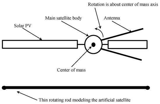
Figure 1.
Artificial satellite modeled as thin rod.
In this context, several real artificial satellites could be modeled as a thin rotating rod since their width is neglected compared to their length. Among these satellites is the Hubble Space Telescope, which has a length of 13.2 m and a maximum diameter of 4.2 m. In addition, the International Space Station (ISS) has a length of 109 m, and the average diameter of its core, where the laboratories are located, is 8 m. Furthermore, some telecommunication satellites are 7 m in length, which is extended by 50 m solar panels, such as GSAT-12R.
The artificial satellite is initially rotating around a principal axis containing the center of mass. This satellite might be hit by space debris. Thus, the rotation axis is modified, and the inertia moment is changed; this could drive the artificial satellite into a chaotic motion, as displayed in Figure 2. This chaotic motion might be the origin of other dangerous space accidents.
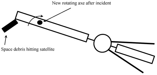
Figure 2.
Artificial satellite changing rotation axis after being hit by space debris.
The resulting and studied mechanical system is presented in Figure 3. This mechanical system is composed of a thin rod represented by a segment and a movable axis represented by point A. The thin rod with normalized length 1 rotates around axis A. The thin rod is subject to an external force, which is gravity.
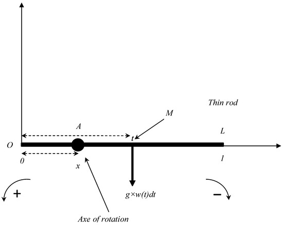
Figure 3.
Studied mechanical system.
2.2. Problem Formulation
As indicated in Figure 3 and for a selected point M from the thin rod, the coordinates of A and M are denoted x and t, respectively. The thin rod mass density function is denoted , then the inertia moment of M about axis A is expressed as follows:
with the elementary mass of point M and the square distance separating points A and M. Since , then the total inertia moment of the thin rod about axis A is given by the following expression:
It is worth noting that for a continuous mass density function , the total inertia moment is also expressed as:
where , , and . This is a direct consequence of extending Equation (1).
The inertia moment is an important parameter in controlling the rotational motion (mechanic, mechatronics, aerospace [40]). In this study, the first parameter controlling the inertia moment is the position of the rotation axis (x), and the second parameter is fixing coefficients a, b, and c (given in (2)).
These coefficients are selected in a way that they depend on the extremities’ values and . Seeking simplicity, this dependence is linear, i.e.,
This choice allows controlling the total inertia moment value by acting on the extremities of the thin rod (or the extremities of the artificial satellite). This action could be performed, for example, by moving a mass to the extremities using actuators [39].
The selection of a, b, and c is based on some physical and mathematical considerations. The whole procedure allowing this section is presented below.
Remark 1.
For a continuous mass density function in , the inertia moment is derivable, and its derivative is: . Thus,
Observe that in (4) represents the total torque for the gravity force (with normalized gravity acceleration ) of the thin rod about axis . This torque is linear, and coefficients a and b are selected such that a linear interpolation of in 0 and 1 is equal to . Figure 4 exhibits the way the linear interpolation is performed.
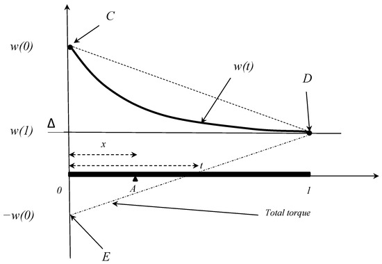
Figure 4.
Linear interpolation for the total torque.
In this case, the equation of line is equal to . Therefore,
Since the inertia moment satisfies for all and , then coefficient c satisfies the following expression: ( is a quadratic expression).
According to (3), , where and are two reals to be determined.
Thus,
Observe that if and , then the two first elements in the previous expression (6) are strictly negative. In this case, and are selected as and . These are the two least integers satisfying the previous conditions ( and ).
Substituting the two latter values in (6), then . Since , then if and only if , which means that:
and
Equations (5) and (7) allow obtaining the coefficients a, b, and c. These coefficients are given as follows.
According to (1), (2), and (9), an integral equation is obtained and expressed as follows.
where the unknown function to be determined is over interval .
Observe that the right-hand side of (10) is the excitation, which is controlled by the values of at the extremities 0 and 1. The left side of the same equation is the response.
The integral Equation (10) is a non-classic integral equation (to the best of our knowledge). The general expression is given as follows.
where:
- The kernel , for .
- is the unknown decreasing and continuous function in .
- , , and are linear forms defined on the continuous functions’ space . The respective expressions are: , , and .
Remark 2.
An obvious solution of (11) is , which was not considered in this study. To avoid such a solution, the unknown mass density function was assumed to satisfy the following additional condition.
This choice did not impact the final solution, as will be shown later. In addition, since represents a mass density function, then
In order to take into account the asymmetry of the artificial satellite, the mass density function was assumed to satisfy:
Remark 3.
A constant mass distribution , , where , is not a solution of integral Equation (11).
Proof.
By contradiction, assume that is a solution of (11), then . The identification term by term yields , which is in contradiction with . □
Remark 4.
Initially, the satellite rotates about the principal axis of the center of mass. After being hit, the artificial satellite might rotate around another axis. Changing the rotation axis from the one of center of mass to another axis may result in a chaotic motion. Several research works studying the artificial satellite chaotic motion, taking into account the inertia moment variation, have been presented [1,2,3,4,5,6,7,8,9,10]. These studies provide mathematical expressions and sufficient conditions allowing the identification of the chaotic motion.
In this study and in order to avoid the chaotic motion, the following expression was adopted and should be minimized as much as possible. This expression is:
where and are the maximum and the minimum inertia moment () values, respectively. These two values exist since the inertial moment function is a continuous function over the compact interval . In other terms,
Assume that, initially, the satellite is rotating about the axis . After being hit by the space debris, the satellite rotates about another axis . The deviation of the inertia moment is then . In order to minimize the risk of a chaotic motion, the latter deviation should be minimized. On the other hand, . In addition, represents the maximum deviation moving from one rotation axis to another one. Consequently, should be minimized to ensure the minimization of . The expression is divided by to relativize it and to obtain a rate within the interval .
Therefore, the expression (15) presents the maximum relative deviation of the inertia moment while varying the rotation axis (x), and we have interest in keeping it as minimum as possible.
Since is quadratic, then:
Trivially, a necessary and sufficient condition to obtain is
This is obtained if . In this case,
2.3. Problem Mathematical Formulation Summary
Based on (11), (12), (13), (14), (17), and (8), a summary of the obtained equations that should be satisfied by the mass density function is presented below.
The objective in the sequel is to find a mass density function satisfying the system (19)–(23).
3. Preliminary Transformations
The integral Equation System (19)–(23) is not a classical one (to the best of our knowledge), and the already-existing methods intended to solve integral equations are not applicable. The aim of this section is to convert the system (19)–(23) into a simpler one. This objective is achieved over several mathematical transformations allowing reaching a simple and equivalent form, which is a nonlinear system.
In this context, a preliminary result is presented in the following proposition (Proposition 1).
Proof.
. The functions , , and are continuous over the compact , Therefore, , , and . In addition, . On the other hand, . The identification term by term gives the previous result (Proposition 1). □
It is worth noting that there is no known procedure to solve System (24)–(26). Therefore, simplifying the integral equation via some transformations is the adopted way to solve it. In this context, an important and well-known result is recalled in the following remark (Remark 5).
Remark 5.
If the mass density unknown function is continuous on the interval , then there exists a unique function defined on and satisfying the following conditions:
- ( is the derivative of ).
The previous result (Remark 5) is about the existence of a unique primitive of such that . In addition, selecting such that is random, and the obtained solution is not impacted by this choice, as will be proven in the remainder of this paper.
The introduction of the function is the beginning of a chain of mathematical transformations allowing the simplification of the integral Equation (11). In this context, the first transformation consists of converting (11) into an integro-differential system. A part of this system is composed of linear differential equations. The unknowns in a system of linear differential equations are functions satisfying several linear derivative equations. The reader is referred to [41,42], where an introduction to the linear differential equations system was presented.
3.1. Integro-Differential Equations’ Transformation
The main result allowing the transformation of the integral Equation (11) into integro-differential equations is presented in the following proposition (Proposition 2).
Proposition 2.
Proof.
- If is a solution of (11), then satisfies (25) and (26), and consequently, (33) and (34) are satisfied.
- Since is a primitive of for , then , and in particular, and (32) is satisfied.
Conversely, assume that and are solutions of System (28)–(33):
- Obviously, Equations (25) and (26) are satisfied since satisfies Equations (33) and (34).
□
Equations (28)–(32) form a system of linear differential equations with unknown functions and , which are at the same time the unknown functions of System (28)–(33).
The shape of the general solution of the system of linear differential equations [41,42] suggests that and might have the following form.
where parameters , and are real constants. The determination of the unknown functions and , provided their existence and the satisfaction of (35), requires the determination of , and . Consequently, substituting (35) into the system (28)–(33) is converting the problem into a system of equations where the unknowns are the constants , and . This is the content of the next subsection.
3.2. Non-Linear System (Representation) Transformation
Substituting (35) into (28)–(33) leads to a system of equations where the unknowns are , and . This substitution of (35) follows the same order as in (28)–(33).
First, including (35) in (28) ( ∀) yields ∀. The identification permits obtaining the following two equations.
Second, substituting Equation (35) in Equation (29) yields the following equation.
Third, based on (35), (30), and (31), the following system is obtained.
Fourth, including (35) in (32) gives
Fifth, substituting (35) into (33) leads to four different equations according to the values of and . Indeed, is turned into , where . The closed form of depends on the value of k ( or ). This results in four cases, which are taken into account in the following remark.
Remark 6.
Based on (33) and (35), the four following expressions are obtained:
- Ifand, then Equation (33) is:
- Ifandthen Equation (33) is:
- Ifand, then Equation (33) is:
- Ifand, then Equation (33) is:
Proof.
Two cases have to be considered while calculating the closed form of the integral where . These two cases are and . For the case , an integration by parts ( and ) yields . In the case where , a direct integration leads to .
The four cases (1) and , (2) and , (3) and , and (4) and are listed below:
- If and , then is equivalent to. Then,. Hence, .
- If and then is equivalent to Consequently, , which yields .
- The proof for the case and , is the same as the previous proof with swapping the roles of and
- If and , then (25) is equivalent to , which involves .
□
Remark 7.
Among the four already-mentioned cases, the one considering has to be discarded. This is because in this case, according to (35). Consequently, for all , which is contradicts (30).
The sixth step consists of substituting (35) into (34), resulting in four cases for the expression . These four cases are exhibited in the following remark (Remark 8):
Remark 8.
- Ifand, then Equation (34) is:
- Ifand, then Equation (26) is:
- Ifand, then Equation (26) is:
- Ifand, then Equation (26) is:
Proof.
The results are based on: □
The collection of (40), (41), (42), (38), (39), (36), and (37) gives three systems . These systems depends on both and . For example, system considers the equations and for Case 1 where and .
In addition, the case and is discarded because of Remark 7, and this is the reason for obtaining three systems. The systems are displayed as follows,
where the unknowns to be determined are: , and .
It is worth noting that System (48) presents a strong nonlinearity with the presence of terms , , and .
Remark 9.
Any solution (if it exists) of System (48) satisfies the following condition.
Proof.
Reasoning by contradiction and assuming that , then ( in the fifth equation of (48)) and, consequently, . In addition, since , the sixth equation in (48) yields . Since and (third and fourth equations in (48)), then and , which means that . The conclusion is and , which is impossible; therefore, . □
In the remainder of this paper, , because of the previous remark (Remark 9).
4. Problem Resolution
The aim of this section is the resolution of System (48), which will lead to a solution of the studied integral equation.
4.1. Nonlinear System Resolution
As a first step in the resolution of System (48), the equations are separated into two subsets, where the first one does not contain terms with . The obtained partial system is presented as follows.
For a given (fixed) and , the system (50) is a linear one, with unknowns . This partial system is presented in matrix form as follows.
Since (Remark 9), then the determinant:
The equations in System (48), which contain and , depend on the cases: and , and , and and . These equations are as follows.
In the sequel, each one of the cases , , and is studied separately. In addition, the following notation is adopted.
4.1.1. Case : and
Substitute , , , and given by (52) in Equation (56) for ( and )). The obtained system with unknowns Z and T is presented as follows.
where:
,
,
,
,
,
,
.
Because , , and , the system (58) is well defined. Considering the two first equations in (58), the obtained linear system regarding the two unknowns Z and T has a determinant . The determinant involves or or or . These four cases are considered separately as follows:
- If , then , and the two first equations in System (58) becomeThis means that and , which is impossible.
- If , then and , and the two first equations in System (58) are:Thus, and . Consequently, and , thus , which is impossible since .
- If , then , and the the two first equations in System (58) becomeTherefore, , which is impossible.
- If , then and , and the system (58) becomesThus, and , which means , and this is impossible since .
As a conclusion of studying the four previous cases, the determinant and the two first equations in (58) have a unique solution, which is expressed as follows.
Thus, , then . If , then and at the same time, which is impossible. Therefore,
Equations (62) and (63), are presented in another form allowing the expression of and , respectively, as follows.
In other terms, .
This means that .
Denote
and study the sign of .
Clearly, the sign of requires studying the signof given by the following expression.
The first and second derivative of are, respectively: and . Consequently,
- If , then . This case is impossible since and .
- If , this case is not valid since and .
The conclusion is that for the case : and , there is no feasible solution for System (48).
4.1.2. Case : and
In this case, , , , and , which are already expressed in (52), become:
.
The expressions of , , , , , and suggest that three cases have to be tested. Indeed, these three cases are generated by , , and . In other terms, these cases correspond to , , and :
- If , then the equation of System (67) yields , which is impossible.
- If , then equations , , and of System (67) yield each. Therefore, for , the solution is , and is kept.
- If , then gives . This solution Z is substituted in . Therefore, , and consequently, . In other terms, , which yields . This contradicts the fact that .
The only kept case among the previous three ones is . In this particular case (), System (48) admits a solution expressed as follows.
Consequently, for this case where and , the system (28)–(33) has a solution, which is expressed in the following formula.
4.1.3. Case : and
The same treatment is performed for this case as for the previous one ( and ) because of the symmetry, and
For this particular case, the solution of System (28)–(33) is expressed as follows.
4.1.4. Case and
Remark 7 provides a reason for discarding this case.
As a conclusion, a solution of the integral Equation (11) is:
After exploring the four previous cases, the obtained solution satisfies also:
which means that Condition (20) is satisfied. Furthermore,
This means that Condition (21) is satisfied.
This involves Conditions (22) and (23) being satisfied. Thus, the obtained density mass function is a solution of (19)–(23). Moreover, is too close to , and . This means that (18) is satisfied.
The whole procedure for solving the studied problem is summarized in Algorithm 1 below.
| Algorithm 1 Steps solving the problem for . |
1. The integral Equation (11) is derived. 2. The integral Equation (11) is transformed into the system of integro-differential Equations (28)–(34). 4. The nonlinear systems (48) is solved. |
If some new conditions on the mass density function are included or existing ones are modified, the presented methods still works as long as the obtained system (as the obtained one in this study (48)) has a solution for the unknowns , and . If the obtained system has no solution, then the following expressions (35):
could be slightly modified as follows.
where , , , and are polynomial functions. Indeed, the latter expressions allow more flexibility. If the expression (76) does not work, then the numerical resolution is recommended.
In order to verify experimentally the obtained results, a micro-gravity environment is required. Several scientific experiments requiring a micro-gravity field were carried out in the International Space Station (ISS). Therefore, a rod with the obtained mass density function needs to be sent to the ISS, and the necessary experiments about the chaotic motion have to be conducted.
4.2. Engineering Technical Feasibility of the Obtained Solution
The obtained mass density function is , . This means that while designing an artificial satellite and in order to take into account the risk of incidents with space debris, the mass of the satellite should be well distributed. This could be performed by following certain mass distribution functions. In the current study, the solution is a mass density function suggesting that the mass is concentrated in the extremity and the mass density is rapidly decreasing as we approach the other extremity .
More generally, the material with such a mass distribution function is a kind of a non-homogeneous material, which is indeed manufactured and used in different engineering areas. This material is called Functionally Graded Material (FGM). FGMs are composed of thin superimposed layers ( m: nano material), where each layer is a mix of two different homogenous materials, with different proportions. As an example, FGMs used as a heat shelter are composed of ceramic and metal, as indicated in Figure 5.
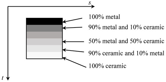
Figure 5.
FGM representation.
Consequently, the physical proprieties (the shear modulus, the mass density function, the heat conductivity, and the thermal expansion coefficient) in these materials (FGMs) exponentially depend on the thickness (t). Therefore, a physical propriety for an FGM material is given by:
where and are positive parameters depending on the FGM [43,44].
Different engineering areas benefit from FGMs and their useful properties. For example, the biomedical area uses FGMs to develop new materials intended to substitute bones and teeth [32,33]. In addition, FGMs are commonly used in the aerospace industry, where new materials are developed to cope with the harsh space environment. The electronic engineering field also uses FGMs in order to provide more accurate components [45].
FGMs’ manufacturing techniques are advancing in a spectacular way, and more efficient and accurate FGMs have been produced during the two last decades. In this context, numerous new engineering techniques are proposed such as: laser deposition, thermal spray, chemical vapor deposition/infiltration, and the surface reaction process [46].
5. Conclusions
In this paper, an artificial satellite was modeled as a thin rotating rod. This satellite might be hit by space debris, and this could drive it into a chaotic motion. In order to avoid this chaotic motion, some physical and mathematical conditions were set. These conditions led to a complicated mathematical system, where the mass density function of the satellite was the unknown to be determined. This system was analytically solved, and the obtained analytical solution for the studied problem was a linear exponential.
This suggests that the mass distribution function of an artificial satellite should be well distributed during the design period, in order to prevent chaotic motion, after being hit by space debris.
Future research has to focus on the uniqueness of the solution of the studied non-classical integral equation. Furthermore, the existence and the resolution of the studied integral equation for other new forms , , and have to be explored. In addition, the 2D and 3D generalizations of the studied problem have to be considered.
Author Contributions
The contributions of authors are as follows: modeling, resolution, and writing, L.H.; modeling and software, M.M.; software, M.A. All authors have read and agreed to the published version of the manuscript.
Funding
This project was funded by the National Plan for Science, Technology and Innovation (MAARIFAH), King Abdulaziz City for Science and Technology, Kingdom of Saudi Arabia, Award Number 15-MAT4882-02.
Institutional Review Board Statement
Not applicable.
Informed Consent Statement
Not applicable.
Data Availability Statement
Not applicable.
Acknowledgments
This project was funded by the National Plan for Science, Technology and Innovation (MAARIFAH), King Abdulaziz City for Science and Technology, Kingdom of Saudi Arabia, Award Number 15-MAT4882-02. The authors also thank the Deanship of Scientific Research and RSSU at King Saud University for their technical support.
Conflicts of Interest
The authors declare no conflict of interest.
References
- Peltoniemi, J.I.; Wilkman, O.; Gritsevich, M.; Poutanen, M.; Raja-Halli, A.; Näränen, J.; Flohrer, T.; Di Mira, A. Steering reflective space debris using polarised lasers. Adv. Space Res. 2021, 67, 1721–1732. [Google Scholar] [CrossRef]
- Schubert, M.; Böttcher, L.; Gamper, E.; Wagner, P.; Stoll, E. Detectability of space debris objects in the infrared spectrum. Acta Astronaut. 2022, 195, 41–51. [Google Scholar] [CrossRef]
- Lanchares, I.V.; Rothos, V.M.; Salas, J.P. Chaotic rotations of an asymmetric body with time-dependent moments of inertia and viscous drag. Int. J. Bifurc. Chaos 2003, 13, 393–409. [Google Scholar]
- Aslanov, V.; Yudintsev, V. Dynamics and chaos control of gyrostat satellite. Chaos Solitons Fractals 2012, 45, 1100–1107. [Google Scholar] [CrossRef]
- Chegini, M.; Sadati, H.; Salarieh, H. Analytical and numerical study of chaos in spatial attitude dynamics of a satellite in an elliptic orbit. Proc. Inst. Mech. Eng. Part C J. Mech. Eng. Sci. 2019, 233, 561–577. [Google Scholar] [CrossRef]
- Iñarrea, M.; Lanchares, V. Chaotic pitch motion of an asymmetric non-rigid spacecraft with viscous drag in circular orbit. Int. J. Non-Linear Mech. 2006, 41, 86–100. [Google Scholar] [CrossRef]
- Jin, R.; Chen, X.; Geng, Y.; Hou, Z. LPV gain-scheduled attitude control for satellite with time-varying inertia. Aerosp. Sci. Technol. 2018, 80, 424–432. [Google Scholar] [CrossRef]
- Aslanov, V.S.; Doroshin, A.V. Chaotic dynamics of an unbalanced gyrostat. J. Appl. Math. Mech. 2010, 74, 524–535. [Google Scholar] [CrossRef]
- Lian, X.; Liu, J.; Zhang, J.; Wang, C. Chaotic motion and control of a tethered-sailcraft system orbiting an asteroid. Commun. Nonlinear Sci. Numer. Simul. 2019, 77, 203–224. [Google Scholar] [CrossRef]
- Kouprianov, V.V.; Shevchenko, I.I. Rotational dynamics of planetary satellites: A survey of regular and chaotic behavior. Icarus 2005, 176, 224–234. [Google Scholar] [CrossRef]
- Kianejad, S.S.; Enshaei, H.; Duffy, J.; Ansarifard, N. Prediction of a ship roll added mass inertia moment using numerical simulation. Ocean. Eng. 2019, 173, 77–89. [Google Scholar] [CrossRef]
- Ochiai, Y. Numerical integration to obtain moment of inertia of nonhomogeneous material. Eng. Anal. Bound. Elem. 2019, 101, 149–155. [Google Scholar] [CrossRef]
- Hirsch, J.E. Moment of inertia superconductors. Phys. Lett. A 2019, 383, 83–90. [Google Scholar] [CrossRef]
- Sun, X.; Zhu, J.; Hanif, A.; Li, Z.; Sun, G. Effects of blade shape and its corresponding inertia moment on self-starting and power extraction performance of the novel bowl-shaped floating straight-bladed vertical axis wind turbine. Sustain. Energy Technol. Assess. 2020, 38, 100648. [Google Scholar] [CrossRef]
- Zhang, J.; Chao, Q.; Xu, B. Analysis of the cylinder block tilting inertia moment and its effect on the performance of high-speed electro-hydrostatic actuator pumps of aircraft. Chin. J. Aeronaut. 2018, 31, 169–177. [Google Scholar] [CrossRef]
- Wazwaz, A.-M. Linear and Nonlinear Integral Equations: Methods and Applications; Springer: New York, NY, USA, 2011. [Google Scholar]
- Malovichko, M.; Khokhlov, N.; Yavich, N.; Zhdanov, M. Acoustic 3D modeling by the method of integral equations. Comput. Geosci. 2018, 111, 223–234. [Google Scholar] [CrossRef]
- Kanaun, S. Integral equations of the crack problem of poroelasticity: Discretization by Gaussian approximating functions. Int. J. Solids Struct. 2020, 184, 63–72. [Google Scholar] [CrossRef]
- Zhu, S.P.; Lin, S.; Lu, X. Pricing puttable convertible bonds with integral equation approaches. Comput. Math. Appl. 2018, 75, 2757–2781. [Google Scholar] [CrossRef]
- Ata, K.; Sahin, M. An integral equation approach for the solution of the Stokes flow with Hermite surfaces. Eng. Anal. Bound. Elem. 2018, 96, 14–22. [Google Scholar] [CrossRef]
- Wei, T.; Xu, M. An integral equation approach to the unsteady convection–diffusion equations. Appl. Math. Comput. 2016, 274, 55–64. [Google Scholar] [CrossRef]
- Shanin, A.V.; Korolkov, A.I. Diffraction by an elongated body of revolution. A boundary integral equation based on the parabolic equation. Wave Motion 2019, 85, 176–190. [Google Scholar] [CrossRef]
- Golub, V.M.; Doroshenko, O.V. Boundary integral equation method for simulation scattering of elastic waves obliquely incident to a doubly periodic array of interface delaminations. J. Comput. Phys. 2019, 376, 675–693. [Google Scholar] [CrossRef]
- Serry, M.; Tuffaha, A. Static stability analysis of a thin plate with a fixed trailing edge in axial subsonic flow: Possio integral equation approach. Appl. Math. Model. 2018, 63, 644–659. [Google Scholar] [CrossRef]
- Li, P. Generalized convolution-type singular integral equations. Appl. Math. Comput. 2017, 311, 314–323. [Google Scholar] [CrossRef]
- Maleknejad, K.; Shahabi, M. Application of hybrid functions operational matrices in the numerical solution of two-dimensional nonlinear integral equations. Appl. Numer. Math. 2019, 136, 46–65. [Google Scholar] [CrossRef]
- Maleknejad, K.; Rashidinia, J.; Eftekhari, T. Numerical solution of three-dimensional Volterra-Fredholm integral equations of the first and second kinds based on Bernstein’s approximation. Appl. Math. Comput. 2018, 339, 272–285. [Google Scholar] [CrossRef]
- Maleknejad, K.; Dehbozorgi, R. Adaptive numerical approach based upon Chebyshev operational vector for nonlinear Volterra integral equations and its convergence analysis. J. Comput. Appl. Math. 2018, 344, 356–366. [Google Scholar] [CrossRef]
- Panigrahi, B.L.; Mandal, M.; Nelakanti, G. Legendre multi-Galerkin methods for Fredholm integral equations with weakly singular kernel and the corresponding eigenvalue problem. J. Comput. Appl. Math. 2019, 346, 224–236. [Google Scholar] [CrossRef]
- Ren, Y.; Zhang, B.; Qiao, H. A simple Taylor-series expansion method for a class of second kind integral equations. J. Comput. Appl. Math. 1999, 110, 15–24. [Google Scholar] [CrossRef]
- Sadri, K.; Amini, A.; Cheng, C. A new operational method to solve Abel’s and generalized Abel’s integral equations. Appl. Math. Comput. 2018, 317, 49–67. [Google Scholar] [CrossRef]
- Suk, M.J.; Choi, S.I.; Kim, J.S.; Kim, Y.D.; Kwon, Y.S. Fabrication of a porous material with a porosity gradient by a pulsed electric-current sintering process. Met. Mater. Int. 2003, 9, 599–603. [Google Scholar] [CrossRef]
- Thieme, M.; Wieters, K.P.; Bergner, F.; Scharnweber, D.; Worch, H.; Ndop, J.; Kim, T.J.; Grill, W. Titanium-powder sintering for preparation of a porous functionally graded material destined for orthopaedic implants. J. Mater. Sci. 2001, 12, 225–231. [Google Scholar]
- Wazwaz, A. The regularization method for Fredholm integral equations of the first kind. Comput. Math. Appl. 2011, 61, 2981–2986. [Google Scholar] [CrossRef]
- Yaman, O.I.; Kress, R. Nonlinear integral equations for Bernoulli’s free boundary value problem in three dimensions. Comput. Math. Appl. 2017, 74, 2784–2791. [Google Scholar] [CrossRef]
- Egidi, N.; Maponi, P.; Quadrini, M. An integral equation method for the numerical solution of the Burgers equation. Comput. Math. Appl. 2018, 76, 35–44. [Google Scholar] [CrossRef]
- Hackbusch, W. Integral Equations: Theory and Numerical Treatment; Birkhauser-Verlag: Basel, Switzerland, 1995. [Google Scholar]
- Burov, A.A.; Kosenko, I.I.; Guerman, A.D. Equilibrium configurations and control of a moon-anchored tethered system. Adv. Astronaut. Sci. 2013, 146, 251–266. [Google Scholar]
- de Matos Lino, M.F.G. Design and Attitude Control of a Satellite with Variable Geometry. Master’s Thesis, Instituto Superior Tecnico, Lisboa, Portugal, 2013. [Google Scholar]
- Zhai, G.; Liang, H.; Liu, M. Position Optimum Analysis of Aerospace Relay’s Pushing Rod. Chin. J. Aeronaut. 2003, 16, 29–35. [Google Scholar] [CrossRef]
- Igor, K.; Pultr, A. Systems of Linear Differential Equations. In Introduction to Mathematical Analysis; Birkhäuser: Basel, Switzerland, 2013; pp. 175–191. [Google Scholar]
- Oberguggenberger, M.; Ostermann, A. Systems of Differential Equations. In Analysis for Computer Scientists; Undergraduate Topics in Computer Science; Springer: London, UK, 2011. [Google Scholar]
- El-Borgi, S.; Hidri, L.; Abdelmoula, R. An embedded crack in a graded coating bonded to a homogeneous substrate under thermo-mechanical loading. J. Therm. Stress 2005, 29, 439–466. [Google Scholar] [CrossRef]
- El-Borgi, S.; Erdogan, F.; Hidri, L. A partially insulated embedded crack in an infinite functionally graded medium under thermo-mechanical loading. Int. J. Eng. Sci. 2004, 42, 371–393. [Google Scholar] [CrossRef]
- Kato, K.; Kurimoto, M.; Shumiya, H.; Adachi, H.; Sakuma, S.; Okubo, H. Application of functionally graded material for solid insulator in gaseous-insulation systems. IEEE Trans. Dielectr. Electr. Insul. 2006, 13, 362–372. [Google Scholar] [CrossRef]
- Naebe, M.; Shirvanimoghaddam, K. Functionally graded materials: A review of fabrication and properties. Appl. Mater. Today 2016, 5, 223–245. [Google Scholar] [CrossRef]


Publisher’s Note: MDPI stays neutral with regard to jurisdictional claims in published maps and institutional affiliations. |
© 2022 by the authors. Licensee MDPI, Basel, Switzerland. This article is an open access article distributed under the terms and conditions of the Creative Commons Attribution (CC BY) license (https://creativecommons.org/licenses/by/4.0/).