Abstract
In engineering applications, where we demand more and more precision, the modeling of systems with hysteretic nonlinearity has received considerable attention. The classical Preisach model (CPM) is currently the most popular for characterizing systems with hysteresis, and this model can represent the hysteresis with an infinite but countable first-order inversion curve (FORC). The table method is a method used to realize CPM in practice. The data in the table corresponds to a limited number of FORC samples. There are two problems with this approach: First, in order to reflect the timing effects of elements with hysteresis, it needs to consume a lot of memory space to obtain accurate data table. Second, it is difficult to come up with an efficient way to modify the data table to reflect the timing effects of elements with hysteresis. To overcome these shortcomings, this paper proposes to use a set of polynomials instead of the table method to implement the CPM. The proposed method only needs to store a small number of polynomial coefficients, and thus it reduces the required memory usage. In addition, to obtain polynomial coefficients, we can use least squares approximation or adaptive identification algorithms, which can track hysteresis model parameters. We developed an adaptive algorithm for the identification of polynomial coefficients of micro-piezoelectric actuators by applying the least mean method, which not only reduces the required memory size compared to the table method implementation, but also achieves a significantly improved model accuracy, and the proposed method was successfully verified for displacement prediction and tracking control of micro-piezoelectric actuators.
1. Introduction
With the development of computer and numerical techniques, the use of hysteresis models has become more and more popular in finite element (FE) method (FEM)-based computer-aided design (CAD) simulations for calculating magnetization properties and iron losses [1]. Hysteresis appears in many engineering devices or smart materials, such as micro-piezoelectric actuators (PZA), piezoelectric ceramics, shape memory alloys (SMA), and ferromagnetic components [2,3,4,5,6], which is a nonlinear phenomenon. Systems with hysteresis are often difficult to describe accurately, and without feedback control, may lead to unstable behavior of the system. When a device exhibits nonlinearity, the system often exhibits inaccuracies or oscillations, even instability caused by the non-differentiable hysteresis and non-memoryless properties of magnetic hysteresis [7,8,9]. Therefore, accurate hysteresis models are crucial for developing suitable control algorithms or applications using these systems [10]. Several models have been developed to characterize systems with hysteresis; commonly used models include the Bouc–Wen, Preisach-like Krasnosel’skii–Pokrovskii (KP), Prandtl–Ishlinskii model (PIM), and the classical Preisach model (CPM) [11]. CPM has long been known as the most familiar model for characterizing hysteretic behavior. It uses double integrals with relay operators and weighting parameters to describe the system input/output relation, which can be further represented by an infinite but countable first-order inversion curve (FORC), which can be experimentally measured in many applications [12]. The traditional method to implement CPM for systems with hysteresis approximate by sampling a finite number of FORCs and storing the sample data in a table [13]. The model output is then evaluated from the table data and the given input by simple linear interpolation. However, this approach has two drawbacks: One is that when the number and sampling resolution of FORC should be increased, it requires a large amount of memory space to accurately predict the hysteresis behavior. The other is that it is difficult to find an efficient way to adjust the data table to reflect changes in parameters with aging or time. As a result, execution accuracy may degrade over time and even require rebuilding of the table.
To overcome these drawbacks, we recommend implementing CPM using a set of polynomials rather than data tables. It only needs to store a small number of polynomial coefficients to reduce the required storage space. Specifically, polynomial coefficients can be obtained using a least squares approximation or an adaptive identification algorithm [14], allowing tracking of hysteresis model parameters. The proposed method has been applied to computer simulations of CPM output predictions. We apply the least mean squares (LMS) adaptation algorithm to develop an adaptive algorithm for identifying the polynomial coefficients of FORC. Compared to the implementation of the table method, the results show that it has higher model accuracy than the table method and requires significantly less memory. Furthermore, the proposed method combined with an adaptive algorithm can achieve dynamic modification of CPM parameters instead of rebuilding the table. According to [15], the proposed method has been applied to simulate the displacement of micro-piezo actuators. The modeled RMS error changes from 1.0098 µm for the table method to 0.4539 µm.
The remainder of this paper is divided to five sections including conclusions. Section 2 reviews the hysteresis and the Preisach model. Section 3 introduces the basic definition and the numerical implementation on the CPM. Section 4 present the computer simulations to verify capabilities of different realizations of the CPM. Section 5 demonstrates the applications of the micro-piezoelectric actuators. The final section presents the conclusions.
2. Realization Numerical of CPM
The classical Preisach model (CPM) [16,17] represents the input and output relations of a system with hysteresis by a double integral formula as below:
where denotes the CPM input, is the CPM output, is the Preisach density function, and is an operator with two distinct outputs. The idea of the CPM is to regard a hysteresis transducer as the superposition of infinitely weighted hysteresis operators as shown in Figure 1.
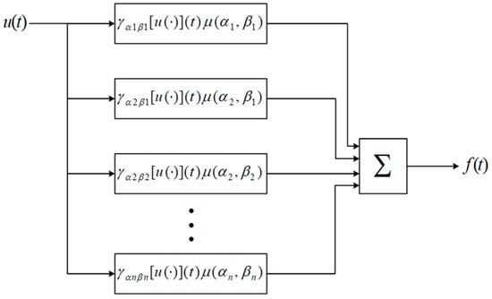
Figure 1.
Architecture of the Preisach model.
The hysteresis operator is the most important core in the Preisach model. The values and of the hysteresis operator correspond to “up” and “down” switching values of input, respectively. In this paper, we assume that . The operator is characterized by its switching values and , which are represented by a rectangular loop on its input and output phase diagrams, as shown in Figure 2. As shown in the figure, the operator output of remains −1 until the input is higher than the value of , and the output remains until the input is lower than the value of . A practical expectation for practical applications is the limit of the integration, which requires us to set the saturation value of the input, that is, .
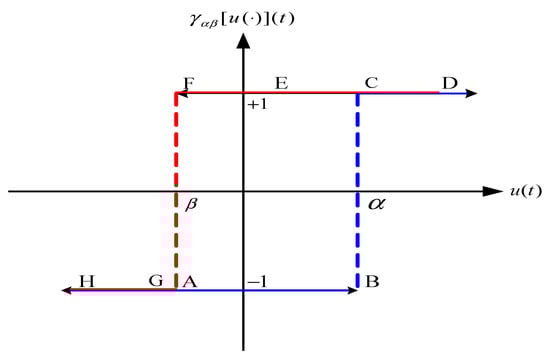
Figure 2.
The hysteresis operator: the output follows trajectory when the input is increasing and follows when the input is decreasing.
A progressive evaluation of the CPM is demonstrated by the following example, depicted in Figure 3. In the example, we calculate a first order reversal curve (FORC), a curve is formed after the first reversal of the input, and a second order reversal curve. Any higher order reversal curve can be constructed by using the analogical method.
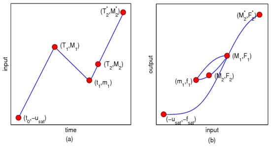
Figure 3.
A progressive evaluation of the CPM: (a) the input diagram; (b) the input–output phase diagram.
Assume the system is first at negative saturation; that is, the CPM input is and all hysteresis operator outputs are . Then, the initial CPM output is
As the CPM input increases from to , the hysteresis operator output will be switched to the if the switching value is less than the current input value . Then, the CPM output is
When the CPM input changes direction and decreases from to a value , the hysteresis operator output will be switched to the state for the switching value greater than . Then, the FORC is
Evaluation of is the same with , that is,
The wiping-out property appears as the input reaching and then reaches . Hysteresis operators with a switching value less than but greater than stay at the state after , so they have no influence on the current output. Additionally, hysteresis operators with greater than but less than are originally at the state and would be transitioned to . Summarizing all of the above,
It is clear that and , which were wiped out, are not necessary to determine in (5).
In the CPM, hysteresis operator is a concern associated with the impact of the past inputs for such scheme. The wiping-out property, however, clarifies that to determine the current CPM the output does not have to memorize all of the history of CPM but only parts of the extremum of the past inputs and outputs [18]. The CPM can be rewritten in such a way to dichotomize a CPM output into two terms: the shifted term, depending on the past outputs, and the integrated term, depending on the past inputs and the current input. We can define alternating series, which are kept to determine the limits of integration and the storage part of a CPM output, by generalizing the above-mentioned example as below. Consider a particular input for a CPM in the time interval and . We use the notations for the time the global maximum of is reached and for the time the global minimum of is reached, where and satisfy that
The alternating series of the input in is defined as a tuple , and the alternating series of the output in is , where and . Furthermore, for a given alternating series and , except at some point, the CPM output is obtained by
If is increasing, and
If is decreasing. In the ensuing discussion, the alternating series except are assumed to be recorded.
So far, we developed forthright mathematical Formulas (8) and (9) to simplify the CPM with the known Preisach density function and given alternating series. However, the identification of requires the differentiation of experimental data, which may amplify errors in the experimental data. There are some algorithms [19,20] published to remove sensitivity of identification of , but the approach using to evaluate CPM outputs is still unappealing. Although we could find an accurate of CPM, the double integration would be very time consuming and mathematically intractable. The congruency property of CPM supplies another way of representing a CPM through use of the FORC to replace integration with experimental data [16]. We introduce the property and how to use FORC to numerically implement a CPM by examining (8) and (9). It is expected that the integrated terms in (8) or (9) for a particular CPM input will be congruent with other CPM input if their limits of integration are the same. Ground on this fact, we can store integrated terms with variational limits of integration beforehand. The FORC measuring experiment is used for this notion. In order to connect FORC and the algebraic calculation of the CPM output, a function is defined as the output of a CPM with and a function is the output of a CPM with . Hence, denotes an ascending FORC and denotes a descending FORC. Thus, (8) is equivalent to
Additionally, (9) is equivalent to
From the above discussion, the numerical implementation of the CPM can be obtained by combining the alternating series and the FORC, which can be used for evaluation of the CPM output; this approach avoids the trouble of differentiation and integration shown in Figure 4.
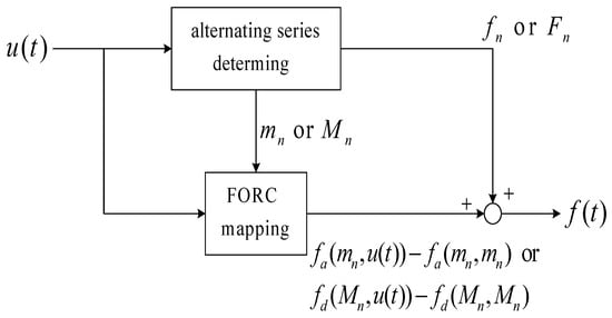
Figure 4.
Block diagram of the numerical implementation of the CPM.
3. Realizations of the CPM
In the previous section, we introduced the basic definition and the numerical implementation on the CPM. We also developed and as an algebraic representation of a CPM. Because the and can be explicitly obtained by experiments of the FORC-measuring experiments, they play the central roles in the realization of a CPM. In practice, however, it is impossible to obtain all values of FORC which requires infinite and uncountable experiments. One realizable method to approximate values of FORC is to find finite data of and , store them as tables, and we can obtain values of or by the interpolation using its neighbors stored in tables. In this section, we take an introductory look at different realizations of a CPM using finite-FORC, including the table method [21,22], polynomial approximation, and adaptive polynomial approximation.
Linear interpolation is a very intuitive way to estimate values between known values and we adopt this method to approximate or . If a point belongs to a rectangular cell formed by , , , , and we have , , , . Then, is approximated by
If a point belongs to a triangular cell formed by , , , then is approximated by
The Formulas (12) and (13) also exist for .
It is convenient to investigate the measured data using an analyzable function called curve fitting and the polynomial function is commonly used. Our goal is to fit the samples of a finite number of FORC using polynomial functions. For instance, we can use a quadratic polynomial function of single variable M to fit with a particular . That is,
Additionally, also can be approximated as
where and are notations to indicate the polynomial coefficients corresponding with and , respectively. The coefficients of the curve fitting method vary with or , so to know all of them is also impossible. Hence, we also use the interpolation to approximate coefficients that are not derived from experiments. For ,
For ,
According to (10) and (11), a CPM output can be determined by a sifted term and a combination of FORC. Now, we substitute for FORC by using (14) and (15). If the input is ascending,
Define , ; for , , then
Thus, (18) becomes
where
Additionally, indicates . Similarly, if the input is descending,
where
Additionally, , . The polynomial coefficients represent the parameters of the CPM and are suitable for model identification because they are adjustable.
Based on the polynomial approximation, we obtain a set of coefficients that can be used to describe FORC. However, these coefficients may not be accurate. For a system model with inaccurate parameters, we can use adaptive algorithms such as LMS or RLS [18] to update the parameters. Compared with the adaptive model output and plant output, this error is used to update adaptive system parameters. Assume the adaptive model output is a function of parameters and the input , and the plant output is a function of the input . Define the error as
The steepest descent algorithm is:
where is a step size. Using (20), (22), (25), we obtain following updated formulations:
If the input is ascending,
If the input is descending,
Then, we can obtain CPM outputs by applying polynomial coefficients adapted by (26) or (27) to (20) or (22).
4. CPM Simulation and Discussion
In this section, we demonstrate the computer simulations to verify capabilities of different realizations of the CPM proposed in Section 3. Consider a special CPM with Preisach density function,
We chose , , , , and in our simulations. The exact CPM outputs are calculated by numerical integral of Matlab. The FORC are measured and sampled in the tables first; these sampled data are used to obtain polynomial coefficients. The CPM outputs are predicted via different realizations and the root mean square error (RMS) is adopted as the judgment of how close the prediction is to the CPM. We can also observe the tracking ability of the adaptive polynomial approximation by disturbing slightly.
To implement the table method, the samples of the ascending FORC and descending FORC are measured first. By dividing into 6 segments, the CPM input is decreased from to some divided point and then increased to . After the input begins decreasing from some divided point to , we sample the CPM outputs every unit change in the CPM input and store these sampling data in Table 1 which presents the samples of ascending FORC. The first column denotes the value of of , and the first row denotes the value of . The samples of descending FORC are stored in Table 2 using a similar procedure and both ascending and descending FORC are plotted in Figure 5.

Table 1.
Sampling data of ascending FORC.
Table 2.
Sampling data of descending FORC.
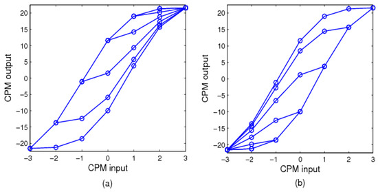
Figure 5.
FORC of the CPM: (a) ascending FORC; (b) descending FORC.
We apply the least-square approximation to sampling data of Table 1 and Table 2 to identify the polynomial coefficients directly in this simulation. Because of the establishment of saturated boundaries, FORC are much more gradual and cannot be fit by polynomials adequately. Hence, and are rejected in the procedure of the least-square approximation and the table method is used if they are needed. The polynomial coefficients are stored in Table 3 and Table 4. Based on (20) and (22), the polynomial coefficients and are not needed for the polynomial approximation. The polynomial coefficients of and are plotted in Figure 6.
Table 3.
Polynomial coefficients of .
Table 4.
Polynomial coefficients of .
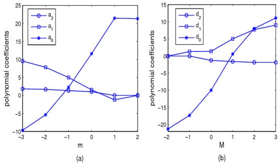
Figure 6.
The coefficients of the PA: (a) of ; (b) of .
In our simulations, we use a sinusoidal CPM input that with a frequency of 1 Hz has a sample time of 0.01 s, and a varying amplitude. The waveform of CPM input and the input–output phase diagram are shown in Figure 7. The simulation results are shown in Figure 8, Figure 9, Figure 10 and Figure 11. The CPM output and CPM output realized via the table method are plotted together in Figure 8a. The difference between these two outputs, defined as the prediction error, are shown in Figure 8b. The RMS of the prediction error is 0.5256. The result of the simulation of the polynomial approximation is shown in Figure 9, and its RMS is 1.0717. We use a step size and Table 3 and Table 4 as initial parameters of the adaptive polynomial approximation and the simulation result is shown in Figure 10. The RMS of the adaptive polynomial approximation is 0.5909. We also plotted these three prediction errors together in Figure 11 for comparison. We can find that the performance of the adaptive polynomial approximation and the table method are in the same range roughly and are better than the polynomial approximation. This is because polynomial approximation uses a single function to characterize a FORC but the table method uses a number of linear functions. The adaptive polynomial approximation, however, adjusts the coefficients of the polynomial so it can be viewed using several functions to fit FORC equivalently and has a better effect than the polynomial approximation.
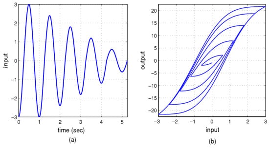
Figure 7.
The CPM input and output of simulations: (a) the waveform of the CPM input; (b) the input–output phase diagram.
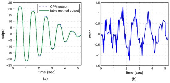
Figure 8.
Prediction of the CPM output using the table method: (a) the CPM output compared with prediction via the table method; (b) the prediction error of the table method.
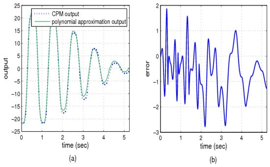
Figure 9.
Prediction of the CPM output using PA: (a) the CPM output compared with prediction via PA; (b) the prediction error of PA.
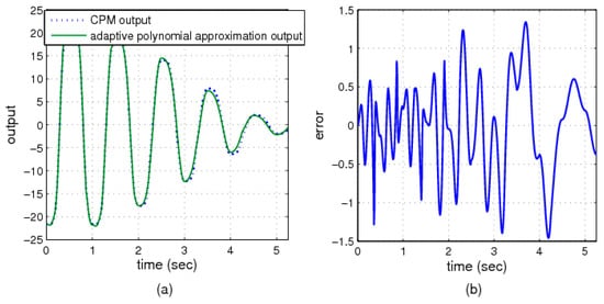
Figure 10.
Prediction of the CPM output using the adaptive PA: (a) the CPM output compared with prediction; (b) the prediction error.
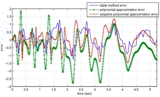
Figure 11.
Prediction error of the CPM via different realizations.
We saw the performance of dissimilar realizations of the CPM with a fixed Preisach density function. That is, we assume that the quality of the CPM is abiding for all situations. This assumption is not cohere with systems in real applications. It is broad that the table method and the polynomial approximation are static models and hard to be modify real time. An advantage of the adaptive polynomial approximation is that the parameters of such scheme are obtained on-line; this means that even if the CPM changed, the adaptive polynomial approximation will trace the CPM by adjusting its parameters. To witness this, we disturb such that becomes from 1.5 to 1.3 and becomes from 1.8 to 2.1. Table 1 and Table 2 are still used to implement the table method; Table 3 and Table 4 are still used to implement the polynomial approximation and are the initial parameters of the adaptive polynomial approximation. We apply the same CPM input of previous simulations and the new CPM output compared with the original CPM output is plotted in Figure 12. Then, we use the different realizations to predict the new CPM output and plot the prediction errors together in Figure 13. The RMS of each realization is 1.9707 for the table method, 1.0746 for the polynomial approximation, and 0.6349 for the adaptive polynomial approximation. It is clear that the adaptive polynomial approximation has the best performance in this simulation.
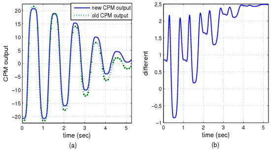
Figure 12.
The CPM output of a changed Preisach density function: (a) the new CPM output compared with the original CPM output; (b) the difference between the new and original CPM output.
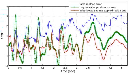
Figure 13.
Prediction error of the CPM of a changed Preisach density function via different realizations.
5. Applications for Piezoelectric Actuators
We use different realizations of Preisach model to predict the displacement of a micro-piezoelectric actuator and the inverse Preisach model introduced in this thesis to control it. In these applications, the input of the Preisach model is actuator voltage and the output of the Preisach model is displacement.
To implement the Preisach model, several first order reversal curves are measured for the micro-piezoelectric actuator first. By dividing 0∼5 V into 10 segments, the input voltage of micro-piezoelectric actuator is increased from 0 V to some divided point and then decreased to 0 V. After the input begins decreasing from some divided point to 0, we sample the displacements of the micro-piezoelectric actuator every 0.45 V change in input voltage and store these sampling data in Table 5. The first column denotes the value of M, and the first row denotes the value of m. In the predication experiment, we use a sinusoidal and input voltage with a frequency of 1 rad/s, an amplitude of 2.25 V, and a bias of 2.25 V; the input and output waveforms of the micro-piezoelectric actuator of the predication experiment are shown in Figure 14, and the phase transition is shown in Figure 15. In the tracking control experiment, we use a sinusoidal desired output with with a frequency of 1 rad/s, an amplitude of 15 µm, and a bias of 16 µm. The sampling time of the experiment is 0.01 s and the total time is 50 s.
Table 5.
Sampling data of FORC.
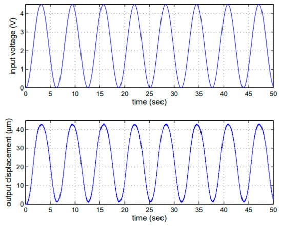
Figure 14.
The input and output of the micro-piezoelectric actuator.
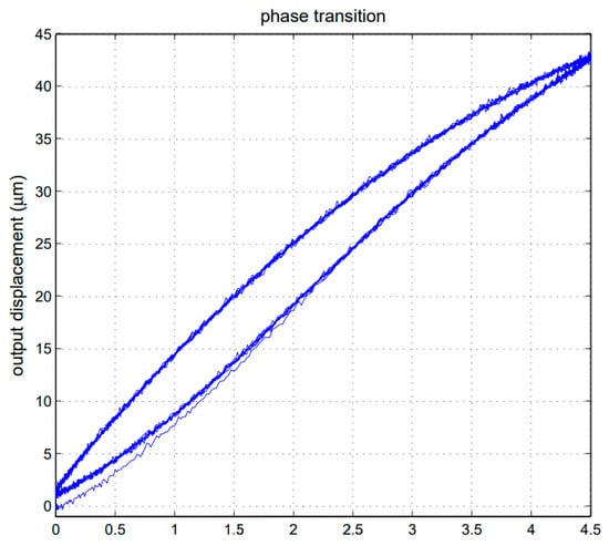
Figure 15.
The phase transition of micro-piezoelectric actuator.
The displacement of the micro-piezoelectric actuator and the output of the Preisach model realized via the table method are plotted together in Figure 16a. The difference between these two outputs, defined as the model error, is shown in Figure 16b. The phase transition of model and of plant are plotted together in Figure 17. The RMS of the model error is 1.0098 µm, and the required amount of memory to store the table is 66.
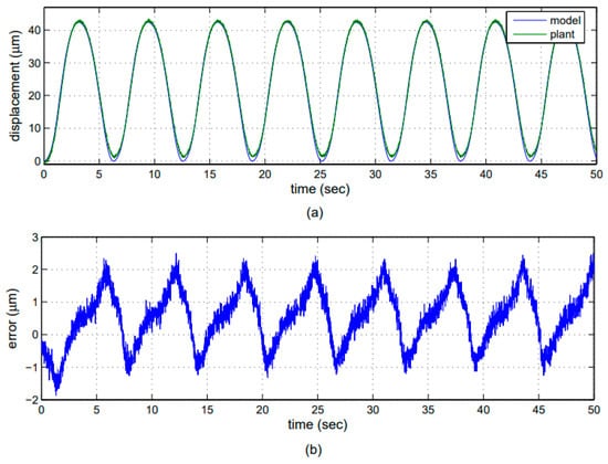
Figure 16.
Prediction of the micro-piezoelectric actuator using the Preisach model realization via the table method: (a) the displacement of the micro-piezoelectric actuator and the output of the Preisach model; (b) the error between these two outputs.
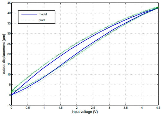
Figure 17.
Phase transition of the micro-piezoelectric actuator using the Preisach model realization via the table method.
We apply the least-square approximation to sampling numbers of Table 5 to identify the polynomial coefficients directly in this experiment. The polynomial coefficients are stored in Table 6. The polynomial coefficient c0 is not needed for the Preisach model realization. The displacement of the micro-piezoelectric actuator is compared with the output of the Preisach model which is realized via the table method as shown in Figure 18a, and the model error is shown in Figure 18b. The phase transition of the model and of the plant are plotted together in Figure 19. The RMS of the model error is 1.4817 µm, and the amount of memory for polynomial coefficients is 22.
Table 6.
The polynomial coefficients.
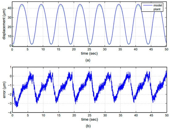
Figure 18.
Prediction of the micro-piezoelectric actuator using the Preisach model realization via polynomial approximation: (a) the displacement of the micro-piezoelectric actuator and the output of the Preisach model; (b) the error between these two outputs.
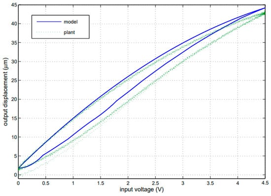
Figure 19.
Phase transition of the micro-piezoelectric actuator using the Preisach model realization via polynomial approximation.
We develop the least mean square (LMS) adaptive algorithm to obtain accuracy polynomial coefficients and the data in Table 6 are used as the initial parameters. We test the step sizes µ = 10 − 4, µ = 10 − 3, and µ = 0.00051 + u(t) and the process of each is shown in Figure 20. The polynomial coefficients obtained by the LMS adaptive algorithm with step size µ = 0.00051 + u(t) are stored in Table 7.
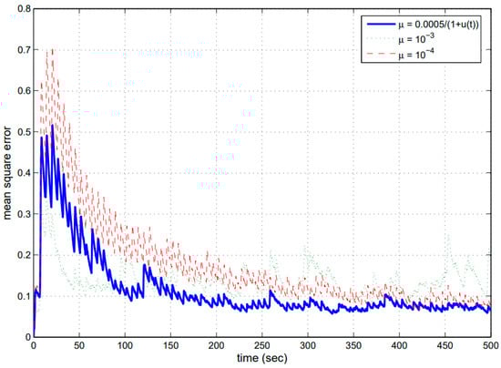
Figure 20.
Mean square error of the prediction of the micro-piezoelectric actuator for varying step-size µ using the adaptive polynomial approximation.
Table 7.
The polynomial coefficients obtained using the LMS adaptive algorithm.
The displacement of the micro-piezoelectric actuator is compared with the output of the Preisach model, which is shown in Figure 21a, and the model error is shown in Figure 21b. The phase transitions of the model and the plant are plotted together in Figure 22. The RMS of the model error is 1.5898 µm.
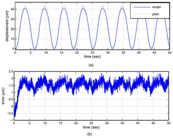
Figure 21.
Prediction of the micro-piezoelectric actuator using the Preisach model realization via the adaptive polynomial approximation: (a) the displacement of the micro-piezoelectric actuator is compared with the output of the Preisach model; (b) the model error.
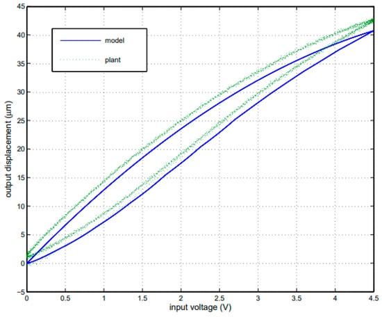
Figure 22.
Phase transition of the micro-piezoelectric actuator using the Preisach model realization via the adaptive polynomial approximation.
Obviously, a bias exists in Figure 21b. This means that the Preisach model should be modified in the beginning of the micro-piezoelectric actuator work. Figure 23 shows the phase transition of the model error and the input in the beginning ascending branch.
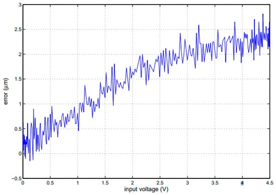
Figure 23.
Phase transition of the model error and the input.
We predict the displacement of the micro-piezoelectric actuator again. The displacement of the micro-piezoelectric actuator is compared with output of the Preisach model which is shown in Figure 21a, and the model error is shown in Figure 24b. The phase transition of the model and the plant are plotted together in Figure 25. The RMS of the model error is 0.4539 µm. The model error of the Preisach model realization via the table method and the modified polynomial approximation are plotted together in Figure 26 for comparison.
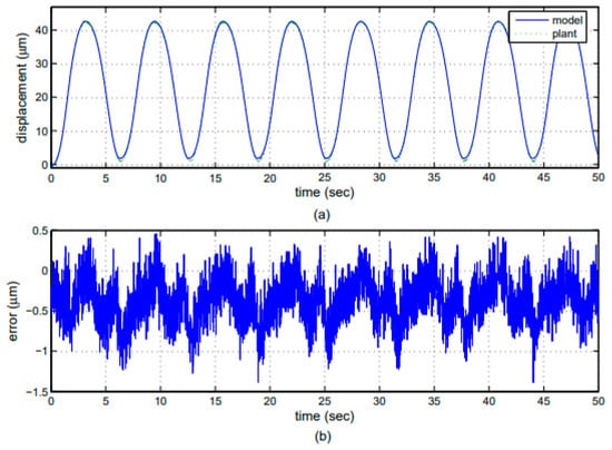
Figure 24.
Prediction of the micro-piezoelectric actuator using the Preisach model realization via the modified polynomial approximation: (a) the displacement of the micro-piezoelectric actuator is compared with output of the Preisach model; (b) the model error.
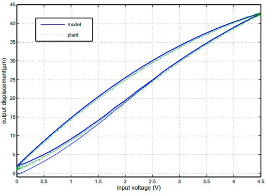
Figure 25.
Phase transition of the micro-piezoelectric actuator using the Preisach model realization via the modified polynomial approximation.
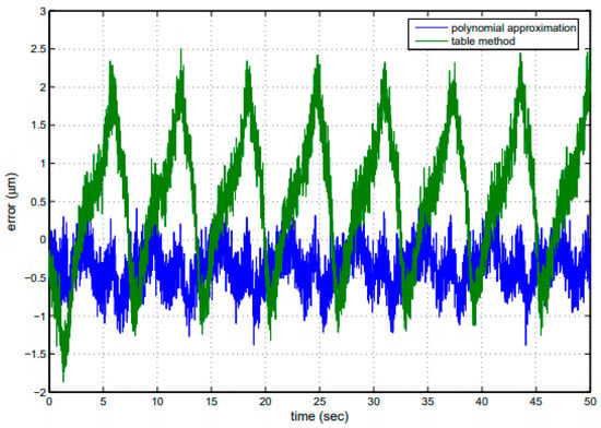
Figure 26.
Model error of the Preisach model realization via the table method and the modified polynomial approximation.
An experimental inverse Preisach model for tracking control of micro-piezoelectric actuators was developed. The desired output compared with the displacement of the micro-piezoelectric of this experiment is plotted together in Figure 27a. The difference between these two outputs, defined as the tracking error, is shown in Figure 27a. The RMS of the tracking error is 0.7079 µm. To reduce tracking error, we combine the inverse Preisach model with a PID controller. The parameters of the PID controller are Kp = 0.0452, Ki = 2.9828, and Kd = 0.0024. The desired output compared with the displacement of the micro-piezoelectric actuator of this experiment are plotted together in Figure 28a. The tracking error is shown in Figure 28b. The RMS of tracking error is 0.2438 µm.
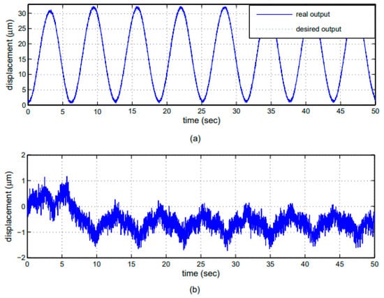
Figure 27.
Tracking of the micro-piezoelectric actuator using the inverse Preisach model: (a) the desired output compared with the displacement of the micro-piezoelectric; (b) the difference between these two outputs.
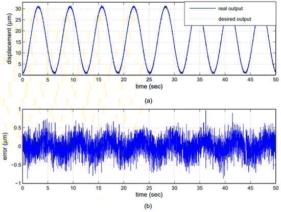
Figure 28.
Tracking of the micro-piezoelectric actuator using the inverse Preisach model with a PID controller: (a) the desired output compared with the displacement of the micro-piezoelectric actuator; (b) the tracking error.
6. Conclusions
We implemented the CPM with a polynomial approximation to characterize the hysteresis. Compared with the traditional table method, this method requires less storage space and enables parameter tracking of the hysteresis element through experiments. We successfully obtained polynomial coefficients to model the CPM with a particular Preisach density function in Section 4, and the polynomial coefficients to model the displacement of a micro-piezoelectric actuator in Section 5. In Section 4, the obtained model compared with that via the table method not only requires less memory but also yields a smaller modeling RMS error from 1.0746 via the table method to 0.6349 as the CPM is changed. In Section 5, the modeling RMS error changed from 1.0098 µm via the table method to 0.4539 µm as CPM changes. We also established the inverse Preisach model based on the polynomial approximation; this model was combined with the PID controller used for tracking control and yielded small tracking RMS error of 0.2438 µm.
Author Contributions
All authors adopted the Preisach model to characterize hysteresis behaviors and proposed to use polynomial approximation to realize the Preisach model; this approach was then used to model the displacement of a real micro-piezoelectric actuator. The proposed approach can overcome the drawbacks of the conventional table method. Finally, all authors have given final approval of the version to be published and agree to be accountable for all aspects of the work in ensuring that questions related to the accuracy or integrity of any part of the work are appropriately investigated and resolved. All authors have read and agreed to the published version of the manuscript.
Funding
This research was sponsored by the Ministry of Science and Technology of Taiwan under the Grant MOST 110-2221-E-150-038.
Acknowledgments
This paper is in memory of Mu-Huo Cheng who was a professor in the Department of Electrical and Control Engineering, National Chiao Tung University, Hsinchu, Taiwan.
Conflicts of Interest
The authors declare no conflict of interest. Moreover, the funders had no role in the design of the study; in the collection, analyses, or interpretation of data; in the writing of the manuscript, or in the decision to publish the results.
Glossary
| u(t) | signal input |
| f(t) | Preisach model output |
| μ(α,β) | Preisach density function |
| hysteresis operator | |
| α(β) | hysteresis operator corresponds to ‘up’ (‘down’) switching values of input |
| divides the range of input data | |
| (τ) | input signal |
| } | peaks of the previous input signal |
| } | valleys of the previous input signal |
| (M,m) | polynomial function |
| (M) | indicates the coefficient corresponding with M |
| (M) | polynomial coefficients |
| represents the effect of previous input | |
| (t) | polynomial approximation |
| (t) | output error |
| f(t) | plant output |
| update algorithm for the vector | |
| T | transpose operation |
| X(t) | function of the input |
| η | constant step size |
| N | normalization factor |
References
- Hussain, S.; Lowther, D.A. An Efficient Implementation of the Classical Preisach Model. IEEE Trans. Magn. 2018, 54, 7300204. [Google Scholar] [CrossRef]
- MacKenzie, I.; Trumper, D.L. Real-Time Hysteresis Modeling of a Reluctance Actuator Using a Sheared-Hysteresis-Model Observer. IEEE/ASME Trans. Mechatron. 2016, 21, 4–16. [Google Scholar] [CrossRef]
- Liang, H.; Zeng, C.; Giraud-Audine, C. Modelling and Simulation of Shape Memory Alloys Micro-Actuator. In Proceedings of the 2009 Fourth International Conference on Innovative Computing, Information and Control (ICICIC), Kaohsiung, Taiwan, 7–9 December 2009; pp. 1405–1408. [Google Scholar]
- Jia, W.; Luo, X.; Chen, X. Modeling and analysis of hysteresis in piezoceramic actuators excited by dynamic driving frequency. In Proceedings of the 2009 Symposium on Piezoelectricity, Acoustic Waves, and Device Applications (SPAWDA 2009), Wuhan, China, 17–20 December 2009; p. 116. [Google Scholar]
- Agrawal, B.N.; Elshafei, M.A.; Song, G. Adaptive antenna shape control using piezoelectric actuators. Act. Astronaut. 1997, 40, 821–826. [Google Scholar] [CrossRef] [Green Version]
- Mayhan, P.; Srinivasan, K.; Watechagit, S.; Washington, G. Dynamic modeling and controller design for a piezoelectric actuation system used for machine tool control. J. Intell. Mater. Syst. Struct. 2000, 11, 771–780. [Google Scholar] [CrossRef]
- Chen, X.; Su, C.; Fukuda, T. Adaptive Control for the Systems Preceded by Hysteresis. IEEE Trans. Autom. Control 2008, 53, 1019–1025. [Google Scholar] [CrossRef]
- Tao, G.; Kokotovic, P.V. Adaptive control of plants with unknown hystereses. IEEE Trans. Autom. Control 1995, 40, 200–212. [Google Scholar] [CrossRef]
- Zhang, J.; Merced, E.; Sepúlveda, N.; Tan, X. Modeling and Inverse Compensation of Nonmonotonic Hysteresis in VO2-Coated Microactuators. IEEE/ASME Trans. Mechatron. 2014, 19, 579–588. [Google Scholar] [CrossRef]
- Li, Z.; Zhang, X.; Su, C.-Y.; Chai, T. Nonlinear Control of Systems Preceded by Preisach Hysteresis Description: A Prescribed Adaptive Control Approach. IEEE Trans. Control Syst. Technol. 2016, 24, 451–460. [Google Scholar] [CrossRef]
- Riccardi, L.; Naso, D.; Turchiano, B.; Janocha, H. Adaptive Control of Positioning Systems with Hysteresis Based on Magnetic Shape Memory Alloys. IEEE Trans. Control Syst. Technol. 2013, 21, 2011–2023. [Google Scholar] [CrossRef]
- Stoleriu, L.; Stancu, A. Using Experimental FORC Distribution as Input for a Preisach-Type Model. IEEE Trans. Magn. 2006, 42, 3159–3161. [Google Scholar] [CrossRef]
- Ge, P.; Jouaneh, M. Modeling hysteresis in piezoceramic actuators. Prec. Eng. 2005, 17, 211–221. [Google Scholar] [CrossRef]
- Liu, V.-T.; Lin, C.-L.; Wing, H.-Y. New realisation of Preisach model using adaptive polynomial approximation. Int. J. Syst. Sci. 2012, 43, 1642–1649. [Google Scholar] [CrossRef]
- Liu, V.-T.; Lin, C.-L.; Wing, H.-Y. Realization of Preisach model using adaptive polynomial approximation method. In Proceedings of the 2010 5th IEEE Conference on Industrial Electronics and Applications, Taichung, Taiwan, 15–17 June 2010; pp. 1258–1263. [Google Scholar]
- Mayergoyz, I.D. Mathematical Models of Hysteresis; Springer: New York, NY, USA, 1991. [Google Scholar]
- Mayergoyz, I.D. Hysteresis models from the mathematical and control theory points of view. J. Appl. Phys. 1985, 57, 3803–3805. [Google Scholar] [CrossRef]
- Choi, S.B.; Han, Y.M. Hysteretic behavior of a magnetorheological fluid: Experimental identification. Acta Mech. 2005, 180, 37–47. [Google Scholar] [CrossRef]
- Iyer, R.V.; Shirley, M.E. Hysteresis Parameter Identification with Limited Experimental Data. IEEE Trans. Magn. 2004, 40, 3227–3239. [Google Scholar] [CrossRef]
- Tan, X.; Baras, J.S. Adaptive Identification and Control of Hysteresis in Smart Materials. IEEE Trans. Autom. Control 2005, 50, 827–839. [Google Scholar]
- Ge, P.; Jouaneh, M. Tracking control of a piezoceramic actuator. IEEE Trans. Control Syst. Technol. 1996, 4, 209–216. [Google Scholar]
- Tang, Z.-H.; Lv, F.-U.; Xiang, Z.-H. Hysteresis model of magnetostrictive actuators and its numerical realization. J. Zhejiang Univ. Sci. A 2007, 8, 1059–1064. [Google Scholar] [CrossRef]
Publisher’s Note: MDPI stays neutral with regard to jurisdictional claims in published maps and institutional affiliations. |
© 2022 by the authors. Licensee MDPI, Basel, Switzerland. This article is an open access article distributed under the terms and conditions of the Creative Commons Attribution (CC BY) license (https://creativecommons.org/licenses/by/4.0/).