A CNN-MPSK Demodulation Architecture with Ultra-Light Weight and Low-Complexity for Communications

Abstract

Modulation is an indispensable component in modern communication systems and multiple phase shift keying (MPSK) is widely studied to improve the spectral efficiency. It is of great significance to study the MPSK modulations of symmetric phases in practice. Based on convolutional neural networks (CNNs), we propose a generic architecture for MPSK demodulation, referred to as CNN-MPSK. The architecture utilizes a single-layer CNN and a pooling trick to crop network parameters. In comparison with conventional coherent demodulation, the CNN-MPSK eliminates three modules, i.e., carrier multiplication, bandpass filter and sampling decision. Thus, we can avoid $\pi$-inverted phenomenon from the multiplication of two carrier waves with different phases, as the carrier multiplication is not employed. In addition, we can reduce errors introduced by sampling decision. Furthermore, we conduct bit-error-rate tests for binary-PSK, 4PSK, 8PSK, and 16PSK demodulation. Experimental results reveal that the performance of CNN-MPSK is almost the same to that of conventional coherent demodulation. However, the CNN-MPSK demodulation reduces computational complexity from $\mathit{O}\left(n^2\right)$ to $\mathit{O}\left(n\right)$ as compared to the latter one. Additionally, the proposed scheme can be readily applied for demodulation of non-symmetric MPSK constellations that maybe distorted by linear and nonlinear impairments in communication systems.

1. Introduction

Modulation and demodulation techniques play an important role in data transmission. Original digital signals in communication systems may contain low-frequency components that are difficult to transmit directly through channels. Therefore, the original signals must be encoded onto high-frequency carrier signals for transmission. The encoded process is referred to as modulation [1]. The primary purpose of modulation is to match the frequency bandwidths between signals and channels [2]. Another purpose is to facilitate channel multiplexing [3]. Thus, after modulation, each signal is shifted to a different frequency band so that mutual interference will not occur during transmission. In particular, a multiple phase shift keying (MPSK) demodulation is used to convey data by changing the phase of a constant frequency reference signal. MPSK is a classic modulation that is practically displaced in the standard within orthogonal frequency-division multiplexing (OFDM) symbols for wireless communications. For instance, 4PSK is widely utilized in code division multiple access mobile communications, digital video broadcasting-satellite-second generation communications, coherent optical communications and fiber optic communications. The constellations of MPSK signals are symmetric and zero-mean that is widely used for wireless local area networks and Bluetooth communications.

Recently, a lot of research related to modulation recognition have been undertaken using deep learning technology [4,5,6]. In particular, deep residual networks was investigated to perform radio signal classification, taking into account the effects of carrier frequency offset, symbol rate, and multipath fading. The traditional convolutional neural networks (CNNs) achieve similar performance to residual networks, but with the increased trainable parameters [7]. A novel two-step training for CNN-based automatic modulation classification (CNN-AMC) was then proposed in order to handle complex tasks [8]. Simulation results indicate that the CNN-AMC approximates the optimal maximum likelihood (ML)-AMC. Regarding inference speed, the deep learning-based approach is more than a hundred times faster than ML-AMC by using parallel computation. The relatively simple neural network architectures were presented for space-time-block-codes multiple-input multiple-output systems (MIMO), which are sparse autoencoders-based deep neural networks (DNN) and radial basis function networks (RBFN) [9]. RBFN and DNN weights are optimized using the Broyden–Fletcher–Goldfarb–Shannon algorithm and the least square approach. For the classification of digitally modulated signals in varying channel conditions, Ali and Yang [10] proposed a fully linked two-layer feed-forward DNN with layerwise unsupervised pretraining. This system uses multiple hidden nodes and independent autoencoders for learning feature maps. The proposed DNN has good classification accuracy even when trained and tested at different signal-to-noise ratios (SNRs). To be more efficient in low SNR conditions, the deep belief network and spiking neural network were utilized to reduce execution latency associated with deep learning architectures [11]. Each feature-based AMC classifier is then studied to determine the upper and lower performance bounds within this adaptive framework.

By employing a CNN-based technique, an intelligent eye-diagram analyzer was proposed to recognize modulation formats and estimate optical SNR [12]. Aided by oscilloscope in simulation, the eye diagram images of four modulation formats can be obtained over a wide optical SNR range. It was showed that CNN achieves higher accuracy than other machine learning algorithms such as decision trees, k-nearest neighbors, back-propagation neural networks, and support vector machines. Using the strengths of the CNN and the long short-term memory (LSTM), the AMC is developed by dual-stream construction, which efficiently explores the feature interaction and spatial–temporal properties of raw complex temporal signals [13]. In particular, the signals first go through preprocessing to be converted to the temporal inphase/quadrature format and amplitude/phase representation. To improve modulation recognition accuracy at low SNRs, an algorithm for pre-denoising was proposed in [14] before modulation recognition. The pre-denoising algorithm consists of a fully CNN, which is similar to an auto-encoder. A residual learning is also used to speed up the learning process. Eye diagram measurements were further used to estimate coherent channel performance with deep learning [15]. The experimental results show that the proposed technique provides high accuracy in determining the modulation format, optical SNR, roll-off factor, and timing skew of a quadrature amplitude modulation. In [16], the modulation signals are transformed into two image representations of cyclic spectra and constellation diagram, respectively.

To integrate the features, a gradient descent strategy and a multi-feature fusion technique were exploited along with a two-branch CNN model. The novel framework was proposed for low-cost link adaptation for spatial modulation MIMO (SM-MIMO). Simulations demonstrate that the supervised-learning classifiers and DNN-based adaptive SM-MIMO outperform a variety of conventional optimization-driven designs [17]. The detection of modulations was presented for multi-relay cooperative MIMO systems of 5G communications in the presence of spatially correlated channels and imperfect channel state information. The simulation results show that the machine learning techniques provide gain in terms of both the modulation detection and complexity [18]. To blindly detect the modulation order of interference signals in downlink non-orthogonal multiple access systems, a machine learning algorithm based on Anderson–Darling test was investigated [19]. DNNs and machine learning were used to develop methods for monitoring optical performance, identifying modulation formats, multipath fading channels and orthogonal frequency-division multiplexing supported by compressed sensing assisted index modulation [20,21,22,23].

The previous related studies have yielded positive results. However, these studies utilize deep learning networks, which are deep and have a large output latency [24,25]. As the deep networks have a high degree of complexity, they are difficult to train and generate a large number of parameters, which is unsuitable for small embedded hardware systems. Several studies require the input data of a system to be in an image format. In such case, the received binary data have to be converted into images, and then feature extraction and other operations are carried out. Finally, the image is converted back into binary data. The exchange of binary data and images increases the delay and complexity. There are concerns regarding the system ability to process the received data in real time. Other studies perform pre-processing operations, which increases the amount of parameters and the complexity of the overall system [26,27]. Thus, it is hard to apply these studies for practical hardware implementations. Consequently, based on CNN and pooling techniques, we propose a shallow CNN-MPSK demodulation with ultra-light parameters to achieve a low complexity architecture. The goal of using CNNs with MPSK is to provide an alternative method for demodulation with the affordable computation complexity.

The sections of the study are organized as follows. In Section 2, we analyze the modulation principle of MPSK and the coherent demodulation process. In addition, the theoretical bit-error-rate (BER) formula for coherent demodulation is derived. Section 3 presents the architecture of CNN-MPSK and the computation consumed by each component. We then show the number of parameters generated by the CNN-MPSK architecture. In Section 4, we give a specific CNN-MPSK demodulation example to illustrate parameters training and perform BER tests under different SNRs. Afterwards, we discuss the multiplications and additions involved in CNN-MPSK and coherent demodulation, and conclude this paper in Section 5.

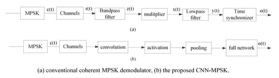
2. Conventional Modulation and Demodulation of MPSK

MPSK is one of the most widely used techniques due to its relative simplicity in modulation and demodulation. The modulation of such signals can be represented by

$$\begin{array}{cc}\hfill & c_i\left(t\right)=\sqrt{\frac{2}{T_c}}sin(w_{c}t+\theta ),\hfill \\ \hfill & \theta =2\pi i/\phantom{2\pi iM}M,i=\{0,1,2,\dots ,M-1\},\hfill \end{array}$$

(1)

where $T_c$ is the period of modulated signal $c_i\left(t\right)$, $T_c=\frac{2\pi }{w_c}$, $w_c$ and $\theta$ denote frequency and phase of the carrier, respectively.

The MPSK demodulation process typically consists of two BPSK demodulation. Figure 1 illustrates the simple case of coherent demodulation for BPSK [28,29]. First, the received BPSK signal $r\left(t\right)$ is filtered to eliminate out-of-band noise using a bandpass filter. Afterwards, the filtered output $z\left(t\right)$ is multiplied by a sin wave $2sin\left(w_{c}t\right)$, resulting in an output $x\left(t\right)$ that is twice the frequency of the input signal. The high frequency components in $x\left(t\right)$ are removed by the lowpass filter. The signal is then passed to the decision circuit. Based on the synchronized clock in the timing synchronizer module, we obtain the final result $o\left(t\right)$ which recovers the binary data stream. In particular, the key component in BPSK demodulation is the carrier generator. It needs to yield a local carrier with the identical frequency and phase as the input signal $r\left(t\right)$. However, the local carrier may not be properly generated, leading to a phase difference between the generated carrier and the received carrier, resulting in negative consequences for demodulation [30,31,32].

Figure 2 depicts the two conditional probability density functions (PDF) $f_0\left(x\right)$ and $f_1\left(x\right)$ for the transmitted bits 0 and 1 with mean values of $\sqrt{2/\phantom{2T_c}{T}_c}$ and $-\sqrt{2/\phantom{2T_c}{T}_c}$, respectively.

In the event that the bit 1 is transmitted and the receiver determines it as 0, the conditional probability of such an error is defined by

$$\begin{array}{cc}\hfill P(0/1)& ={\int }_0^{+\infty }{f}_1\left(x\right)dx\hfill \\ \hfill & ={\int }_{\frac{\sqrt{2/\phantom{2T_c}{T}_c}}{\sqrt{2}{\sigma }_n}}^{\infty }\frac{1}{\sqrt{\pi }}exp[-u^2]du\hfill \end{array}$$

(2)

where

$$\begin{array}{c}\hfill u=\frac{(x+\sqrt{2/\phantom{2T_c}{T}_c})}{\sqrt{2}{\sigma }_n}.\end{array}$$

(3)

The lower limit of integration in Equation (2) is simplified to

$$\begin{array}{c}\hfill \frac{\sqrt{2/\phantom{2T_c}{T}_c}}{\sqrt{2}{\sigma }_n}=\frac{\sqrt{1/\phantom{1T_c}{T}_c}}{\sqrt{N_{0}B}}=\frac{\sqrt{1/\phantom{1T_c}{T}_c}}{\sqrt{N_0/\phantom{N_0{T}_c}{T}_c}}=\frac{1}{\sqrt{N_0}}=\sqrt{\frac{E_b}{N_0}}=\sqrt{snr},\end{array}$$

(4)

where $E_b$ is already normalized to one when BPSK signals are transmitted. Consequently, in terms of the complementary error function (erfc), assuming bits are equiprobable, the BER for BPSK coherent detection is given by

$$\begin{array}{c}\hfill P_e=\frac{1}{2}P(0/1)+\frac{1}{2}P(1/0)=\frac{1}{2}\mathrm{erfc}\left(\sqrt{snr}\right).\end{array}$$

(5)

Similarly, the probability of symbol error of MPSK ($M\ge 4$) is overbounded by [33]

$$\begin{array}{cc}\hfill P_e& =\frac{2}{\sqrt{\pi N_0}}{\int }_{\sqrt{E_s}sin\left(\frac{\pi }{M}\right)}^{\infty }exp[\frac{-x^2}{N_0}]dx\hfill \\ \hfill & =\frac{2}{\sqrt{\pi }}{\int }_{\sqrt{\frac{E_s}{N_0}}sin\left(\frac{\pi }{M}\right)}^{\infty }exp[-u^2]du\hfill \\ \hfill & =erfc[\sqrt{\frac{E_s}{N_0}}sin(\frac{\pi }{M})],\hfill \end{array}$$

(6)

where $\sqrt{E_s}$ is the average energy of the transmitted symbols.

3. The Proposed CNN-MPSK Architecture

3.1. Architecture Presentation

In Figure 3, the proposed architecture takes the received signal as input and then applies one-dimensional (1D) convolution to extract features. Afterwards, the signal flows to the activation module to become unlinear. The flow continues to input a pooling component, followed by a full connection to act as a classifier on the features.

Next, we present the components of the CNN architecture, which consist of 1D convolution, activation, pooling, and full connection. Among these modules, convolution is the most important one. From a mathematical standpoint, convolution can be regarded as an integral operation, or an accumulation. Convolution has the property that past data have an effect on future data, and adjacent data influence current data, which makes convolution convenient to extract features from data. Given a sequence r of length d as input and a vector w of length k, the 1D convolution operation is given by

$$\begin{array}{c}\hfill y\left(m\right)=\sum _k^{}r(m+k)w\left(k\right).\end{array}$$

(7)

The Equation (7) involves element-by-element multiplication and summation. In particular, the elements of vector w are called weights that the network needs to learn during training. Thus, the w is often interchangeably referred to as kernel. Typically, the kernels have small size. In this study, the size of kernel w is 1 × 3, and the 1D output vector z is given by

$$\begin{array}{c}\hfill z\left(j\right)=y+b=\sum _{i=0}^{2}r(j+i)w\left(i\right)+b,0\le j\le d-3,\end{array}$$

(8)

where $z\left(j\right)$ is the j-th element of the output, the z is also referred as extracted feature, and b is called bias which represents the baseline when all the inputs have values of zero. Note that the length of $z\left(j\right)$ is $d-2$. In order to make $z\left(j\right)$ to have the same size as the input r, we add one zero to the first and last positions of r, respectively, which produces a new input vector $r^{\prime }$ = [ 0 r 0]. Thus, we can rewrite Equation (8) as

$$\begin{array}{c}\hfill z^{\prime }\left(j\right)=\sum _{i=0}^2{r}^{\prime }(j+i)w\left(i\right)+b,0\le j\le d-1.\end{array}$$

(9)

The Equation (9) can be illustrated by Figure 4, which gives a visual explanation of how 1D convolution works. In Figure 4, the convolution multiplies the kernel w by the first three elements of $r^{\prime }$, sums all the multiplications with b, and yields the first output $z^{\prime }\left(0\right)$. Following this, we shift the kernel w one element to the right and perform convolution to generate another output $z^{\prime }\left(1\right)$. In particular, the $r^{\prime }\left(0\right)$, $r^{\prime }\left(1\right)$, $r^{\prime }\left(d\right)$ and $r^{\prime }(d+1)$ are equal to zero, $r\left(0\right)$, $r(d-1)$ and zero, respectively. Thus, the first two items $z^{\prime }\left(0\right)$ and $z^{\prime }\left(1\right)$, and the last item $z^{\prime }(d-1)$ are computed as

$$\begin{array}{cc}\hfill z^{\prime }\left(0\right)& =r^{\prime }\left(0\right)w\left(0\right)+r^{\prime }\left(1\right)w\left(1\right)+r^{\prime }\left(2\right)w\left(2\right)+b\hfill \\ \hfill & =r^{\prime }\left(1\right)w\left(1\right)+r^{\prime }\left(2\right)w\left(2\right)+b\hfill \\ \hfill & =r\left(0\right)w\left(1\right)+r\left(1\right)w\left(2\right)+b,\hfill \end{array}$$

(10)

$$\begin{array}{cc}\hfill z^{\prime }\left(1\right)& =r^{\prime }\left(1\right)w\left(0\right)+r^{\prime }\left(2\right)w\left(1\right)+r^{\prime }\left(3\right)w\left(2\right)+b\hfill \\ \hfill & =r\left(0\right)w\left(0\right)+r\left(1\right)w\left(1\right)+r\left(2\right)w\left(2\right)+b,\hfill \end{array}$$

(11)

and

$$\begin{array}{cc}\hfill z^{\prime }(d-1)& =r^{\prime }(d-1)w\left(0\right)+r^{\prime }\left(d\right)w\left(1\right)+r^{\prime }(d+1)w\left(2\right)+b\hfill \\ \hfill & =r^{\prime }(d-1)w\left(0\right)+r^{\prime }\left(d\right)w\left(1\right)+b\hfill \\ \hfill & =r(d-2)w\left(0\right)+r(d-1)w\left(1\right)+b.\hfill \end{array}$$

(12)

It is noted that when the input data change, these three parameters, $w\left(0\right)$, $w\left(1\right)$ and $w\left(2\right)$, do not change. We need to repeat the movement $d-1$ times. This 1D convolution costs $3d$ multiplications and d additions in total.

Following by 1D convolution, there is an activation function that performs nonlinear transformation and enables the neural network to learn nonlinear features. CNNs commonly use rectifier linear units (ReLUs) as activating functions. A ReLU can lead to rapid computation with a threshold value 0. When the input is smaller than 0, the output is 0. Otherwise, the output is unchanged. Applying ReLU, the output can be represented as

$$\begin{array}{c}\hfill f\left(j\right)=max[0,z^{\prime }\left(j\right)],0\le j\le d-1.\end{array}$$

(13)

The pooling is often performed after activation for sub-sampling features. In general, the reason to subsample is that the an important feature of a sequence is seldom contained in adjacent data. The sub-sampling can produce features that are invariant to scale, translation, pose, and rotation changes. Max pooling selects the maximum value from the adjacent data, and thus we have

$$\begin{array}{c}\hfill p\left(m\right)=max\left\{f\right[ms:(m+1)s-1\left]\right\},0\le m\le d/\phantom{ds}s-1,\end{array}$$

(14)

where s is the slide step size and p is the output from max pooling. To provide classification results, a full connection needs to integrate useful and hierarchical features. In a full connection, each unit is connected to all the previous input units. The connection can be expressed as a matrix multiplication, i.e.,

$$\begin{array}{c}\hfill o=\sum _{m=0}^{d/s-1}p\left(m\right)w_f\left(m\right)+b_f,\end{array}$$

(15)

where $b_f$ is a parameter known as bias, $w_f$ are weights, and o denotes a single unit. According to Equation (15), we can construct a structure to depict the full connection, as shown in Figure 5. In BPSK demodulation, we only need one output unit represented by bit 1 or 0. Thus, the full connection costs $d/s$ multiplications and $d/s$ additions for one output.

3.2. Parameter Distribution of CNN-MPSK

The CNN-MPSK network architecture is illustrated in

Table 1. The summary of CNN-MPSK structure.

Type of Operation	Input Shape	Output Shape	Size of Kernel	Parameters
convolution	1 × n × 1	1 × n × 1	1 × 3	4
activation	1 × n × 1	1 × n × 1	0	0
pooling	1 × n × 1	1 × $n/2$ × 1	0	0
full connection	1 × $n/2$ × 1	1 × M	M × $n/2$	M × $n/2$ + M

. The network is rather straightforward. Table 1 shows the type of operation, shape of the input and output, and the number of parameters in the operation. The network takes the $1\times n\times 1$ single-channel data sequence as input. The convolution uses one 1 × 3 kernel and requires three weights and a bias. The 1 × n × 1 data are processed by activation. Then, the data are pooled down by a factor of 2, yielding a 1 × $n/2$ × 1 output. Following this, the full connection module converts the 1 × $n/2$ × 1 input to a 1 × M output with a M × $n/2$ kernel. Note that the activation as well as pooling has no parameters because there is nothing to learn. Thus, the total number of parameters is M × $n/2$ + M + 4, which includes M × $n/2$ + 3 weights and 1 + M biases. In particular, for BPSK, the value of M is equal to 1.

4. Comparison between CNN-MPSK and Coherent Demodulation in Terms of Performance and Computational Complexity

4.1. The Accuracy and Loss Curves

The proposed MPSK modulation assumes a sine wave of one period to represent a symbol. As an example, in BPSK modulation, a sine wave of one cycle represents a 0 or a 1. Our proposed modulation can also be applied for communication systems operated at at MHz or GHz. In order to facilitate comparison, we set the carrier frequency to be 300 KHz and sampling frequency is 6 MHz for BPSK, 4PSK, 8PSK and 16PSK demodulations. Thus, the input to the CNN-MPSK network consists of 20 bits. The training process are similar for these four demodulations. We demonstrate the process by using BPSK as an example. The CNN-BPSK network only requires n/2 + 5 = 15 parameters in total. We generate 1 million experimental data at random, half of which is used for training and half for validating. After training the CNN-BPSK network for 15 epochs, we obtain the accuracy and loss curves versus the number of epochs, as shown in Figure 6. The epoch number is on the x-axis, while accuracy and loss are on the y-axis.

The accuracy in Figure 6 takes a value very near 0.95 and the loss is close to 0.15. The training and validating accuracies improve as we train, while the losses decrease. In particular, the four curves change rapidly in the first two epochs, and the top and bottom parts tend to be 0.95 and 0.15, respectively. After the four epoch, the two accuracy curves almost overlap as well as the two loss curves. The training accuracy is stable, leading to a 94.4% accuracy.

4.2. BER Comparison of CNN-MPSK and Coherent Demodulation

This part presents the demodulation performance of CNN-MPSK. In this experiment, the SNR is snr_db = [−5, −4, −3, −2, −1, 0, 1, 2, 3, 4, 5, 6, 7, 8, 9] in decibels. We need to restore the snr_db to the initial value and perform ${10}^{{}^{\left(snr\_db/10\right)}}$ conversion. We utilize additive white Gaussian noise (AWGN) to simulate channel interference. The tested data for each SNR is 5 million bits, so the total number of noised data flows to CNN-MPSK network is 100 million. With the trained parameters, we predict the noised data and thus obtain the demodulated curve for BPSK, 4PSK, 8PSK and 16PSK, as shown in Figure 7. The blue BER curve is obtained by coherent demodulation. The horizontal axis represents the SNR in dB, while the vertical axis is the BER. The BER curves of the four demodulations from the CNN structure overlap heavily with those based on the conventional coherent demodulation.

4.3. Comparison of Multiplications and Additions

The coherent approach for MPSK involves phase demodulation, requiring linear-phase filters and stable outputs. Therefore, finite impulse response (FIR) filters are preferred. We are concerned with linear-phase FIR filters. The output of an this filter only depends on the present and previous inputs, which can be completely described by

$$\begin{array}{cc}\hfill y\left(n\right)& =\sum _{k=0}^{L-1}{g}_{k}x(n-k)\hfill \\ \hfill & =g_{0}x\left(n\right)+g_{1}x(n-1)+\dots +g_{L-1}x(n-L+1),\hfill \end{array}$$

(16)

where $x\left(n\right)$ is the input sequence of length N, $g_k$ denotes filter coefficients and L represents the FIR filter length. FIRs have no feedback and have stability and freedom from phase distortion. Each coefficient requires a register to hold a delayed input. With the length L of this filter and the N input samples, the length of output $y\left(n\right)$ is $N+L-1$. This process involves $(N+L-1)L$ multiplications and $(N+L-1)(L-1)$ additions [34,35,36]. Consequently, the corresponding computational complexity of an FIR filter is described as $\mathit{O}\left(n^2\right)$.

According to Equation (16), when the length of the received signal is N and the bandpass filter has $L_p$ coefficients, the operation of the bandpass filter costs $(N+L_p-1)L_p$ multiplications and $(N+L_p-1)(L_p-1)$ additions. The carrier multiplier module requires N multiplications. Moreover, let $L_f$ represent the length of the lowpass filter coefficients, the operation of this filter involves $(N+L_f-1)L_f$ multiplications and $(N+L_f-1)(L_f-1)$ additions. As a result, the coherent demodulation involves the total calculations, i.e., $(N+L_p-1)L_p+N+(N+L_f-1)L_f$ = $N(L_p+L_f+1)+L_p^2+L_f^2-(L_p+L_f)$ multiplications, and $(N+L_p-1)(L_p-1)+(N+L_f-1)(L_f-1)$ = $N(L_p-1)+N(L_f-1)+{(L_p-1)}^2+{(L_f-1)}^2$ additions. Demodulating the same input signal as the coherent demodulation, we utilize the proposed CNN-BPSK architecture. In the architecture, the convolution operation requires $3N$ multiplications and N additions, and the full connection needs $N/s$ multiplications and $N/s$ additions, and s is the length of strides. The architecture involves $3N+N/s$ multiplications and $N+N/s$ additions in total.

In comparison with the conventional demodulation, the number of multiplications and additions of the architecture are greatly reduced, as shown in

Table 2. The comparison of calculation between coherent and CNN demodulation.

Type of Demodulation	Multiplications	Additions	Complexity
coherent	$N(L_p+L_f+1)+$ $L_p^2+L_f^2-(L_p+L_f)$	$N(L_p-1)+N(L_f-1)+$ ${(L_p-1)}^2+{(L_f-1)}^2$	$\mathit{O}\left(n^2\right)$
CNN-BPSK	$3N+N/s$	$N+N/s$	$\mathit{O}\left(n\right)$

. The calculation complexity of the proposed demodulation is $\mathit{O}\left(n\right)$, while that of the conventional demodulation is $\mathit{O}\left(n^2\right)$.

Table 3. The comparison of the proposed algorithms and others.

Type of Algorithms	Parameters	Multiplications	Additions	−5 dB	0 dB	10 dB
our CNN BPSK	10	10	10	78.6%	92%	99.9%
our CNN 4PSK	10	10	10	50.9%	70.8%	99.8%
our CNN 8PSK	10	10	10	24%	40.9%	99%
our CNN 16PSK	10	10	10	12%	21.8%	61.6%
ResNet BPSK [7]	${10}^5$	${10}^7$	${10}^7$	50%	97%	99%
ResNet 4PSK [7]	${10}^5$	${10}^7$	${10}^7$	7%	70%	99%
ResNet 8PSK [7]	${10}^5$	${10}^7$	${10}^7$	7%	25%	99%
ResNet 16PSK [7]	${10}^5$	${10}^7$	${10}^7$	6%	40%	85%
DBN BPSK [11]	${10}^2$	${10}^3$	${10}^3$	75%	97%	99%
DBN 4PSK [11]	${10}^2$	${10}^3$	${10}^3$	60%	80%	99%
CNN based BPSK [11]	${10}^5$	${10}^6$	${10}^6$	61%	90%	99%
CNN based 4PSK [11]	${10}^5$	${10}^6$	${10}^6$	50%	75%	99%

presents a comparison between the proposed deep learning technique and the existing algorithms [7,11]. We approximate the number of parameters, and the number of operations by orders of magnitude. The last three columns of Table 3 represent the demodulation accuracy for different $E_s/n0$. The proposed technique shows the similar demodulation performance as compared to the other schemes, but benefits from much reduced implementation complexity, i.e., much less operations and parameters to be trained.

5. Conclusions

This paper proposes a simplified and light-weight CNN-MPSK demodulation architecture based on deep learning technology. The proposed CNN-MPSK can be implemented without requiring the carrier synchronization and timing synchronization that make the system complex. Thus, the design complexity can be greatly reduced and the inverse $\pi$ phenomenon is avoided. The simulation tests are conducted on BER performance of the proposed CNN structure for 4PSK, 8PSK and 16PSK, respectively. We see that the proposed CNN-MPSK shows the similar performance to the coherent demodulation and the existing deep learning demodulations. More importantly, the CNN-MPSK structure has the advantage of greatly reduced computational complexity. As compared with the coherent demodulation, the computation complexity of the proposed architecture is reduced from $\mathit{O}\left(n^2\right)$ to $\mathit{O}\left(n\right)$. Thus, the proposed architecture can be seen as an alternative scheme for low-complexity signal demodulation in communications.

References

1. Koh, K.; Mortazavi, S.Y.; Afroz, S. Time Interleaved RF Carrier Modulations and Demodulations. IEEE Trans. Circuits Syst. I Regul. Pap. 2014, 61, 573–586. [Google Scholar] [CrossRef]
2. Harper, A.D.; Reed, J.T.; Odom, J.L.; Lanterman, A.D.; Ma, X. Performance of a Linear-Detector Joint Radar-Communication System in Doubly Selective Channels. IEEE Trans. Aerosp. Electron. Syst. 2017, 53, 703–715. [Google Scholar] [CrossRef]
3. Abd El-Rahman, A.I.; Cartledge, J.C. Evaluating the Impact of QAM Constellation Subset Selection on the Achievable Information Rates of Multidimensional Formats in Fully Loaded Systems. J. Lightw. Technol. 2018, 36, 712–720. [Google Scholar] [CrossRef]
4. Wang, Y.; Liu, M.; Yang, J.; Gui, G. Data-driven deep learning for automatic modulation recognition in cognitive radios. IEEE Trans. Veh. Technol. 2019, 68, 4074–4077. [Google Scholar] [CrossRef]
5. Njoku, J.N.; Morocho-Cayamcela, M.E.; Lim, W. CGDNet: Efficient hybrid deep learning model for robust automatic modulation recognition. IEEE Netw. Lett. 2021, 3, 47–51. [Google Scholar] [CrossRef]
6. Wang, T.; Hou, Y.; Zhang, H.; Guo, Z. Deep learning based modulation recognition with multi-cue fusion. IEEE Wirel. Commun. Lett. 2021, 10, 1757–1760. [Google Scholar] [CrossRef]
7. O’Shea, T.J.; Roy, T.; Clancy, T.C. Over-the-air deep learning based radio signal classification. IEEE J. Sel. Top. Signal Process. 2018, 12, 168–179. [Google Scholar] [CrossRef] [Green Version]
8. Meng, F.; Chen, P.; Wu, L.; Wang, X. Automatic modulation classification: A deep learning enabled approach. IEEE Trans. Veh. Technol. 2018, 67, 10760–10772. [Google Scholar] [CrossRef]
9. Shah, M.H.; Dang, X. Low-complexity deep learning and RBFN architectures for modulation classification of space-time block-code (STBC)-MIMO systems. Digit. Signal Process. 2020, 99, 102656. [Google Scholar] [CrossRef]
10. Ali, A.; Fan, Y. Unsupervised feature learning and automatic modulation classification using deep learning model. Phys. Commun. 2017, 25, 75–84. [Google Scholar] [CrossRef]
11. Ghasemzadeh, P.; Banerjee, S.; Hempel, M.; Sharif, H. A novel deep learning and polar transformation framework for an adaptive automatic modulation classification. IEEE Trans. Veh. Technol. 2020, 69, 13243–13258. [Google Scholar] [CrossRef]
12. Wang, D.; Zhang, M.; Li, Z.; Li, J.; Fu, M.; Cui, Y.; Chen, X. Modulation format recognition and OSNR estimation using CNN-based deep learning. IEEE Photonics Technol. Lett. 2017, 29, 1667–1670. [Google Scholar] [CrossRef]
13. Zhang, Z.; Luo, H.; Wang, C.; Gan, C.; Xiang, Y. Automatic modulation classification using CNN-LSTM based dual-stream structure. IEEE Trans. Veh. Technol. 2020, 69, 13521–13531. [Google Scholar] [CrossRef]
14. Liu, Y.; Liu, Y. Modulation recognition with pre-denoising convolutional neural network. Electron. Lett. 2020, 56, 255–257. [Google Scholar] [CrossRef]
15. Zhang, Y.; Ren, Y.; Wang, Z.; Liu, B.; Zhang, H.; Li, S.A.; Fang, Y.; Huang, H.; Bao, C.; Pan, Z.; et al. Eye diagram measurement-based joint modulation format, OSNR, ROF, and skew monitoring of coherent channel using deep learning. J. Light. Technol. 2019, 37, 5907–5913. [Google Scholar] [CrossRef]
16. Wu, H.; Li, Y.; Zhou, L.; Meng, J. Convolutional neural network and multi-feature fusion for automatic modulation classification. Electron. Lett. 2019, 55, 895–897. [Google Scholar] [CrossRef]
17. Yang, P.; Xiao, Y.; Xiao, M.; Guan, Y.L.; Li, S.; Xiang, W. Adaptive spatial modulation MIMO based on machine learning. IEEE J. Sel. Areas Commun. 2019, 37, 2117–2131. [Google Scholar] [CrossRef]
18. Chikha, H.B.; Almadhor, A.; Khalid, W. Machine Learning for 5G MIMO Modulation Detection. Sensors 2021, 21, 1556. [Google Scholar] [CrossRef]
19. Zhang, N.; Cheng, K.; Kang, G. A machine-learning-based blind detection on interference modulation order in NOMA systems. IEEE Commun. Lett. 2018, 22, 2463–2466. [Google Scholar] [CrossRef]
20. Khan, F.N.; Zhong, K.; Al-Arashi, W.H.; Yu, C.; Lu, C.; Lau, A.P.T. Modulation format identification in coherent receivers using deep machine learning. IEEE Photonics Technol. Lett. 2016, 28, 1886–1889. [Google Scholar] [CrossRef]
21. Chen, L.; Chen, P.; Lin, Z. Artificial intelligence in education: A review. IEEE Access 2020, 8, 5264–5278. [Google Scholar] [CrossRef]
22. Khan, F.N.; Lu, C.; Lau, A.P.T. Joint modulation format/bit-rate classification and signal-to-noise ratio estimation in multipath fading channels using deep machine learning. Electron. Lett. 2016, 52, 1272–1274. [Google Scholar] [CrossRef]
23. Liu, H.; Lu, S.; El-Hajjar, M.; Yang, L.L. Machine learning assisted adaptive index modulation for mmWave communications. IEEE Open J. Commun. Soc. 2020, 1, 1425–1441. [Google Scholar] [CrossRef]
24. Ye, N.; Li, X.; Yu, H.; Wang, A.; Liu, W.; Hou, X. Deep Learning Aided Grant-Free NOMA Toward Reliable Low-Latency Access in Tactile Internet of Things. IEEE Trans. Ind. Inform. 2019, 15, 2995–3005. [Google Scholar] [CrossRef]
25. Mohammed, S.A.; Shirmohammadi, S.; Altamimi, S. A Multimodal Deep Learning-Based Distributed Network Latency Measurement System. IEEE Trans. Instrum. Meas. 2020, 69, 2487–2494. [Google Scholar] [CrossRef]
26. Fang, Y.; Bu, Y.; Chen, P.; Lau, F.C.; Al Otaibi, S. Irregular-Mapped Protograph LDPC-Coded Modulation: A Bandwidth-Efficient Solution for 6G-Enabled Mobile Networks. IEEE Trans. Intell. Transp. Syst. 2022; in press. [Google Scholar] [CrossRef]
27. Won, Y.S.; Hou, X.; Jap, D.; Breier, J.; Bhasin, S. Back to the basics: Seamless integration of side-channel pre-processing in deep neural networks. IEEE Trans. Inf. Forensics Secur. 2021, 16, 3215–3227. [Google Scholar] [CrossRef]
28. Mesiya, M.F. Digital Information Transmission Using Carrier Modulation. In Contemporary Communication Systems; Lange, M., Ed.; McGraw-Hill: New York, NY, USA, 2013; pp. 600–610. [Google Scholar]
29. Fang, Y.; Chen, P.; Cai, G.; Lau, F.C.; Liew, S.C.; Han, G. Outage-Limit-Approaching Channel Coding for Future Wireless Communications: Root-Protograph Low-Density Parity-Check Codes. IEEE Veh. Technol. Mag. 2019, 14, 85–93. [Google Scholar] [CrossRef]
30. Safak, M. Optimum Receiver in AWGN Channel. In Digital Communications; Wiley, John Wiley and Sons: West Sussex, UK, 2017; pp. 298–319. [Google Scholar]
31. Chen, P.; Xie, Z.; Fang, Y.; Chen, Z.; Mumtaz, S.; Rodrigues, J.J.P.C. Physical-Layer Network Coding: An Efficient Technique for Wireless Communications. IEEE Netw. 2020, 34, 270–276. [Google Scholar] [CrossRef] [Green Version]
32. Haykin, S. Signaling over AWGN Channels. In Digital Communication Systems; Knecht, J., Ed.; John Wiley and Sons: Hoboken, NJ, USA, 2014; pp. 323–410. [Google Scholar]
33. Haykin, S.; Moher, M. Digital band-pass transmission techniques. In Communication Systems; Hong, S., Melhom, A., Eds.; John Wiley and Sons: Hoboken, NJ, USA, 2009; pp. 313–350. [Google Scholar]
34. Tan, L.; Jiang, J. Finite impulse response filter design. In Digital Signal Processing: Fundamentals and Applications; Merken, S., Ed.; Academic Press: Stanford, CA, USA, 2018; pp. 229–236, 550–558. [Google Scholar]
35. Chen, P.; Wang, L.; Lau, F.C.M. One Analog STBC-DCSK Transmission Scheme not Requiring Channel State Information. IEEE Trans. Circuits Syst. I Regul. Pap. 2013, 360, 1027–1037. [Google Scholar] [CrossRef]
36. Rao, K.D.; Swamy, M.N.S. FIR Digital Filter Design. In Digital Signal Processing: Theory and Practice; Springer: Singapore, 2018; pp. 325–338. [Google Scholar]
Figure 1. Block diagram of a coherent binary-PSK (BPSK) receiver.
Symmetry 14 00873 g001
Figure 2. Conditional bit error probability density functions for BPSK demodulated signals.
Symmetry 14 00873 g002
Figure 3. The architecture of a neural network for MPSK demodulation.
Symmetry 14 00873 g003
Figure 4. The operation of the 1D convolution.
Symmetry 14 00873 g004
Figure 5. The operation of the full connection.
Symmetry 14 00873 g005
Figure 6. A plot of accuracy and loss for the CNN-BPSK network.
Symmetry 14 00873 g006
Figure 7. BER comparisons of CNN-MPSK and coherent demodulation for BPSK, 4PSK, 8PSK and 16PSK demodulations.
Symmetry 14 00873 g007