Conformal Deformation, Monopoles, and Their Application to Control the Measurement, Berry Phase’s Path, and Resonant Frequency of a Spin

Abstract

The effects of the conformal deformation of physical parameters on the measurement, Berry phase, and resonance of a spin are investigated. We first construct a form-invariant yet measurement-tunable representation of a spinor from the deformed parameter surface. Then, it is shown that the evolution path of the Berry phase is tunable by the conformal index. Third, the source of the path-tunable Berry phase is shown to be the conformal monopole revealed by the recent investigation of the transformation design of quantum states. The dual fields produced by the dual conformal monopole are presented. It is demonstrated that the strengths of the pole and its dual partner are determined by the reciprocally quantized conformal index. Finally, we discuss the influence of the deformation on the resonance of the spin, and show that the resonant frequency follows the quantization rule ${\overline{\omega }}_R={\omega }_R{\left.\sqrt{\mathrm{conformal}\mathrm{factor}}\right|}_n/n$ with ${\omega }_R$ as the Rabi frequency without deformation.

1. Introduction

A form-invariant solution is generated from a transformation that can maintain the form of the solution to an equation in the original untransformed space but with new variables. In recent years, there has been interest in applying it to design novel devices (e.g., [1,2]). A way to obtain the solution is through conformal mapping. For a 2D system, a suitable mapping not only produces the solution but also offers us freedom to inspect the system’s response when all the variables execute the conformal deformation. Inspired by a conformal monopole and surface revealed from an exploration of the form-invariant solution to the charge-monopole system [3], the purpose of this paper is to report an application of the conformal deformation and the quantization condition of the pole strength to control the measurement, evolution path of the Berry phase, and resonant frequency of a spin in the 2D spherical parameter space.

This paper is arranged as follows: In Section 2, starting with the Hamiltonian of an electron’s spin coupling to a conformal vector in the parameter space, the eigenstates are shown to have the form-invariant representation of the common spinor. The new representation possesses an additional degree of freedom depicted by the conformal index that can be used to tune the outcome of the measurement of the spin along the specific axes. In Section 3, the Berry phase of the spinor generated by an adiabatic transportation of the spin along the conformal coordinate paths is evaluated. It is found that the phase is tunable by the index at the different latitude of the Bloch sphere. A rotating magnetic field is suggested to construct the conformal vector and obtain the Berry phase. In Section 4, the source of the Berry phase is investigated. We show that the phase is established by going around the conformal monopole in the parameter space. In Section 5, we present the dual fields of the dual conformal monopole, and show that the strengths of the pole and its dual partner are dictated by the reciprocally quantized conformal index. Section 6 is used to discuss the resonant phenomenon of the spin on the conformal parameter surface. The resonant frequency associated with the conformal deformation is given. Finally, a conclusion and two remarks are made in the Section 7.

2. Form-Invariant Representation of a Spinor

Instead of the common unit vector ${\widehat{n}}_1=(sin\theta cos\phi ,sin\theta sin\phi ,cos\theta )$, $0\le \theta \le \pi$ and $0\le \phi <2\pi$, in the parameter space used to describe a physical field, we adopt the conformal unit vector ${\widehat{n}}_2=(sin\overline{\theta }cos\overline{\phi },sin\overline{\theta }sin\overline{\phi },cos\overline{\theta })$ to discuss the behavior of a spin coupled to a field by the Hamiltonian $\widehat{H}=\overrightarrow{\sigma }·{\widehat{n}}_2$ where $\overrightarrow{\sigma }$ is the vector formed by the Pauli matrices. The definition of the conformal variables $(\overline{\theta }$, $\overline{\phi })$ is given by the transformation [3]

$$cos\overline{\theta }=\frac{{(1+cos\theta )}^a-{(1-cos\theta )}^a}{{(1+cos\theta )}^a+{(1-cos\theta )}^a},\mathrm{and}\overline{\phi }=a\phi ,$$

(1)

where a is a constant, and can be regarded as a real number. Figure 1 and Figure 2 show the graphs of $cos\overline{\theta }$ and $sin\overline{\theta }$ for some values of a. They are periodic functions with the range $[-1,1]$ and $[0,1]$ except for the trivial case $a=1$ for the latter. The locations of the extreme values of these functions coincide with those given by $cos\theta$ and $sin\theta$. An interesting feature of the function is that $cos\overline{\theta }$ ($sin\overline{\theta }$) is an anti-symmetric (symmetric) function with respect to the negative value of a. The line element for the surface can be expressed as

$$d{\overline{s}}^2=d{\overline{\theta }}^2+{sin}^2\overline{\theta }d{\overline{\phi }}^2={\left({\overline{\theta }}^{\prime }\right)}^{2}d{s}^2,$$

(2)

where

$${\overline{\theta }}^{\prime }=\frac{d\overline{\theta }}{d\theta }=\frac{2a{(sin\theta )}^{a-1}}{{(1+cos\theta )}^a+{(1-cos\theta )}^a},$$

(3)

and $d{s}^2=d{\theta }^2+{sin}^2\theta d{\phi }^2$ is the line element of the common 2D unit sphere $S^2$. Equation (2) exhibits that the surface with the conformal factor ${\left({\overline{\theta }}^{\prime }\right)}^2$ is conformal to $S^2$. Hereafter we shall use ${\overline{S}}^2$ to label the conformal surface. Since the deformation of ${\overline{S}}^2$ is depicted by a, it will be referred to as the conformal index.

Figure 1. (Color online) The graphs show the deformation of $cos\overline{\theta }$ with the conformal index a in a period. The value $a=1$ corresponds to the common cosine function of the plane geometry. The bottom graph shows that the function is antisymmetric with respect to the negative value of a.

Figure 2. (Color online) The graph shows how the sine function with the conformal variable $\overline{\theta }$ deforms with the positive values of the index a, where $a=1$ corresponds to the curve of the common sine function. The function $sin\overline{\theta }$ is a symmetric function with respect to a and $-a$.

It is known that a spin state is described by the spinor $\left|\mathrm{\Psi }\right.⟩$ which can be obtained by evaluating the solution of the Schrödinger equation $\widehat{H}\left|\mathrm{\Psi }\right.⟩=\lambda \left|\mathrm{\Psi }\right.⟩$ with $\lambda$ being the eigenvalue. The condition of having a non-trivial solution to the equation is determined by the characteristic equation

$$\left|\begin{array}{cc}\left(cos\overline{\theta }-\lambda \right)& sin\overline{\theta }{e}^{-i\overline{\phi }}\\ sin\overline{\theta }{e}^{+i\overline{\phi }}& \left(-cos\overline{\theta }-\lambda \right)\end{array}\right|=0.$$

(4)

It gives $\lambda =\pm 1$ and the corresponding normalized spinors,

$$\left|{\mathrm{\Psi }}_{+}\right.⟩=\left(\begin{array}{c}cos\overline{\theta }/2\\ sin(\overline{\theta }/2)e^{i\overline{\phi }}\end{array}\right),\mathrm{for}\lambda =+1,$$

(5)

and

$$\left|{\mathrm{\Psi }}_{-}\right.⟩=\left(\begin{array}{c}sin(\overline{\theta }/2)e^{-i\overline{\phi }}\\ -cos\overline{\theta }/2\end{array}\right),\mathrm{for}\lambda =-1.$$

(6)

They maintain the form-invariance of the familiar spinors. Nevertheless, the conformal degree of freedom allows us to tune the measurement of the spin along the different directions by the index a. For instance, the measurements along the positive and negative z directions of spin for an electron with the spin state $\left|{\mathrm{\Psi }}_{+}\right.⟩$ give the amplitudes

$$⟨{\chi }_{1/2}\left(S_z\right)|{\mathrm{\Psi }}_{+}⟩=cos\overline{\theta }/2,$$

(7)

and

$$⟨{\chi }_{-1/2}\left(S_z\right)|{\mathrm{\Psi }}_{+}⟩=e^{i\overline{\phi }}sin\overline{\theta }/2,$$

(8)

where $\left|{\chi }_{1/2}\left(S_z\right)\right.⟩={(1,0)}^T$ and $\left|{\chi }_{-1/2}\left(S_z\right)\right.⟩={(0,1)}^T$ are the eigenstates corresponding to the eigenvalues $\lambda =+1$ and $-1$ of the Pauli matrix ${\sigma }_z$. Therefore, the probabilities of the spin in the measurements along the $\pm z$ directions are respectively given by

$${\left|⟨{\chi }_{1/2}\left(S_z\right)|{\mathrm{\Psi }}_{+}⟩\right|}^2=\frac{1}{2}\left(1+cos\overline{\theta }\right),$$

(9)

and

$${\left|⟨{\chi }_{-1/2}\left(S_z\right)|{\mathrm{\Psi }}_{+}⟩\right|}^2=\frac{1}{2}\left(1-cos\overline{\theta }\right).$$

(10)

They are independent of $\overline{\phi }$. The graphs in Figure 3 show the probability $P_z(+)\equiv {\left|⟨{\chi }_{1/2}\left(S_z\right)|{\mathrm{\Psi }}_{+}⟩\right|}^2$ which is manipulable by the index a, and the probabilities corresponding to a and $-a$ are complementary. This implies that one can control the probability through the modulation of the index a. The spin orientation of a prepared state $\left|{\mathrm{\Psi }}_{+}\right.⟩$ in the laboratory will almost definitely collapse to the z (negative z) direction in a measurement when the variable $0\le \theta <\pi /2$ ($\pi /2<\theta \le \pi$) if the index value $a>20$. The average of the two measurements above is ${⟨{\sigma }_z⟩}_{+}=cos\overline{\theta }$ which can also be tuned by the index. Analogously, the probabilities of the spin state $\left|{\mathrm{\Psi }}_{+}\right.⟩$ to appear in the $\pm x$, and $\pm y$ directions are given by

$${\left|⟨{\chi }_{1/2}\left(S_x\right)|{\mathrm{\Psi }}_{+}⟩\right|}^2=\frac{1}{2}\left(1+sin\overline{\theta }cos\overline{\phi }\right),$$

(11)

$${\left|⟨{\chi }_{-1/2}\left(S_x\right)|{\mathrm{\Psi }}_{+}⟩\right|}^2=\frac{1}{2}\left(1-sin\overline{\theta }cos\overline{\phi }\right),$$

(12)

and

$${\left|⟨{\chi }_{1/2}\left(S_y\right)|{\mathrm{\Psi }}_{+}⟩\right|}^2=\frac{1}{2}\left(1+sin\overline{\theta }sin\overline{\phi }\right),$$

(13)

$${\left|⟨{\chi }_{-1/2}\left(S_y\right)|{\mathrm{\Psi }}_{+}⟩\right|}^2=\frac{1}{2}\left(1-sin\overline{\theta }sin\overline{\phi }\right).$$

(14)

Figure 3. (Color online) The probability $P_z(+)={\left|⟨{\chi }_{1/2}\left(S_z\right)|{\mathrm{\Psi }}_{+}⟩\right|}^2$ of a spin with the form-invariant state $\left|{\mathrm{\Psi }}_{+}\right.⟩$ in a measurement along the positive z direction. The transverse variable $\theta$ labels the polar angle on the Bloch sphere. The dash-dotted (solid) lines show the tunable behavior of the probability by the conformal index $a=n$$(a=-n),$$n=1,2,3,\cdots$. The probabilities corresponding to $\pm n$ are complementary at a specific $\theta$ angle.

They retain the form-invariance to the common representation. The graphs in Figure 4 show the probability $P_x(+)\equiv {\left|⟨{\chi }_{1/2}\left(S_x\right)|{\mathrm{\Psi }}_{+}⟩\right|}^2$ of the state $\left|{\mathrm{\Psi }}_{+}\right.⟩$ appearing in the positive x direction, where we choose $\phi =\pi /4$ to inspect the outcome. Owing to the conformal freedom, the outcome of a measurement for $\left|{\mathrm{\Psi }}_{-}\right.⟩$ can be realized by the measurement of $\left|{\mathrm{\Psi }}_{+}\right.⟩$ with the negative index $-a$, and vice versa.

Figure 4. (Color online) The probability $P_x(+)={\left|⟨{\chi }_{1/2}\left(S_x\right)|{\mathrm{\Psi }}_{+}⟩\right|}^2$ of the state $\left|{\mathrm{\Psi }}_{+}\right.⟩$ in the positive x direction. The azimuth $\phi =\pi /4$ was chosen to exhibit the dependence of the probability on the conformal index $a=n$. The higher n makes the probability more definite around $\theta =\pi /2$, which reduces its randomness.

3. Controlling the Evolution Path of the Berry Phase

In this section, we first show that the Berry phase of the spin along the conformal coordinate paths depends on the deformation, and the accumulating process of the phase is tunable by the conformal index. Then, a physical realization of the control through a time-dependent rotational magnetic field is suggested. The Berry phase for a normalized, non-degenerate eigenstate $\left|{\mathrm{\Psi }}_n\left(\mathbf{x}\right)\right.⟩$ is defined by (e.g., [4,5])

$${\displaystyle \gamma ={\oint }_C{A}_{\mu }d{x}^{\mu }\mathrm{with}{A}_{\mu }\left(x\right)=-i⟨{\mathrm{\Psi }}_n\left(\mathbf{x}\right)|{\partial }_{\mu }{\mathrm{\Psi }}_n\left(\mathbf{x}\right)⟩,}$$

(15)

which characterizes the time evolution of the state when the parameter $\mathbf{x}(t)$ in the Hamiltonian $\widehat{H}$ changes along a closed path $C:$$\mathbf{x}(t)$$t\in [0,T]$ with $\mathbf{x}(0)=\mathbf{x}(T)$ in the parameter space, i.e., the evolution state is given by

$$\left|\mathrm{\Psi }\left(T\right)\right.⟩=exp\left(-\frac{i}{\hslash }{\int }_0^{T}dt{E}_n\left(\mathbf{x}(t\right))\right)exp\left[i\gamma \right]\left|\mathrm{\Psi }\left(0\right)\right.⟩,$$

(16)

where $E_n$ is the energy corresponding to the instant state $\left|{\mathrm{\Psi }}_n\left(\mathbf{x}\right)\right.⟩$ that satisfies the Schrödinger equation

$$\widehat{H}\left(\mathbf{x}\right)\left|{\mathrm{\Psi }}_n\left(\mathbf{x}\right)\right.⟩=E_n\left|{\mathrm{\Psi }}_n\left(\mathbf{x}\right)\right.⟩.$$

(17)

Berry pointed out that the phase can be non-integrable (i.e., path-dependent) [4]. Thus, there is an interference effect that is physically observable. Hereafter in the article, we shall refer to $A_{\mu }\left(x\right)$ as the Berry potential. For our consideration of the form-invariant spinors, the Berry potential is given by

$$A_{\overline{\phi }}^{+}=-i⟨{\mathrm{\Psi }}_{+}|{\partial }_{\overline{\phi }}{\mathrm{\Psi }}_{+}⟩=\frac{1-cos\overline{\theta }}{2}.$$

(18)

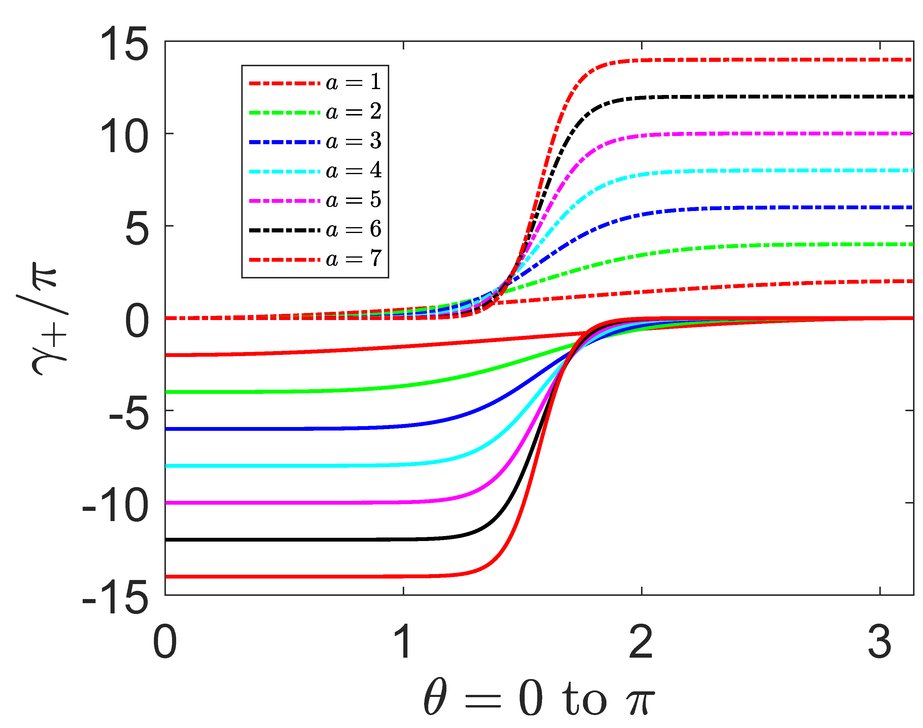
The corresponding Berry phase is

$${\displaystyle {\gamma }_{+}={\oint }_C{A}_{\overline{\phi }}^{+}d\overline{\phi }=a\pi (1-cos\overline{\theta }).}$$

(19)

Figure 5 shows the variation of the phase at the different latitudes on the Bloch sphere. The evolution path at a specific $\theta$ can be altered by the index a. We see that the phase with $a>0$ in the domain $\pi /2<\theta \le \pi$ is complementary to $a<0$ in $0\le \theta <\pi /2$, and the evolution processes of the phase for $a\ne 1$ are allowed drastic changes around $\theta =\pi /2$ which show up different interference patterns. For the other spinor with eigenvalue $\lambda =-1$, we have the Berry potential

$$A_{\overline{\phi }}^{-}=-i⟨{\mathrm{\Psi }}_{-}|{\partial }_{\overline{\phi }}{\mathrm{\Psi }}_{-}⟩=-\frac{(1-cos\overline{\theta })}{2}.$$

(20)

Figure 5. (Color online) The evolution path of the Berry phase of a spin with state $\left|{\mathrm{\Psi }}_{+}\right.⟩$ goes around a conformal monopole. The strength $g=a/2$ of the pole is characterized by the quantized conformal index $a=\pm n$ which can be used to tune the evolution process. The conformal deformation of parameters may result in a drastic variation of the phase around $\theta =\pi /2$ when the index becomes large.

The corresponding Berry phase is

$${\displaystyle {\gamma }_{-}={\oint }_C{A}_{\overline{\phi }}^{-}d\overline{\phi }=-a\pi (1-cos\overline{\theta }).}$$

(21)

This indicates that ${\gamma }_{+}=-{\gamma }_{-}$. Along the closed path of $\overline{\phi }=$ constant, it is easy to show that $A_{\overline{\theta }}^{+}=$$A_{\overline{\theta }}^{-}=0$. Thus, the Berry phase ${\left.{\gamma }_{\pm }\right|}_{\overline{\phi }=\mathrm{constant}}=0$. In the following, let us discuss the gauge freedom of the Berry potential $A_{\overline{\phi }}^{+}$. We rename the state in (5) as

$$\left|{\mathrm{\Psi }}_{+}^{\mathrm{I}}\right.⟩=\left(\begin{array}{c}cos\overline{\theta }/2\\ sin(\overline{\theta }/2)e^{i\overline{\phi }}\end{array}\right)$$

$$\sim \left(\begin{array}{c}1\\ (1-cos\overline{\theta })/sin\overline{\theta }{e}^{-i\overline{\phi }}\end{array}\right)=\left(\begin{array}{c}1\\ (r-\overline{z})/(\overline{x}-i\overline{y})\end{array}\right),$$

(22)

where the Cartesian coordinate system defined by the conformal variables

$$\overline{x}=rsin\overline{\theta }cos\overline{\phi },\overline{y}=rsin\overline{\theta }sin\overline{\phi },\overline{z}=rcos\overline{\theta },$$

(23)

is introduced in the parameter space. It is thus well-defined in the north conformal hemisphere. The corresponding Berry potential is

$$A_{\overline{\phi }}^{\mathrm{I}}=-i⟨{\mathrm{\Psi }}_{+}^{\mathrm{I}}|{\partial }_{\overline{\phi }}{\mathrm{\Psi }}_{+}^{\mathrm{I}}⟩={sin}^2(\overline{\theta }/2).$$

(24)

Another normalized representation of the state $\left|{\mathrm{\Psi }}_{+}\right.⟩$ can be taken as

$$\left|{\mathrm{\Psi }}_{+}^{\mathrm{II}}\right.⟩=\left(\begin{array}{c}cos(\overline{\theta }/2)e^{-i\overline{\phi }}\\ sin\overline{\theta }/2\end{array}\right)\sim \left(\begin{array}{c}(\overline{x}-i\overline{y})/(r-\overline{z})\\ 1\end{array}\right).$$

(25)

It has singularity at the north pole, and good behavior in the south conformal hemisphere. Thus, the conformal deformation of parameters retains the singular behavior of the common spinor (e.g., [5,6]). Two representations in (22) and (25) differ by a gauge transformation, i.e., $\left|{\mathrm{\Psi }}_{+}^{\mathrm{I}}\right.⟩=e^{i\overline{\phi }}\left|{\mathrm{\Psi }}_{+}^{\mathrm{II}}\right.⟩$. The corresponding Berry potential of the state $\left|{\mathrm{\Psi }}_{+}^{\mathrm{II}}\right.⟩$ is

$$A_{\overline{\phi }}^{\mathrm{II}}=-i⟨{\mathrm{\Psi }}_{+}^{\mathrm{II}}|{\partial }_{\overline{\phi }}{\mathrm{\Psi }}_{+}^{\mathrm{II}}⟩=-{cos}^2(\overline{\theta }/2).$$

(26)

Both potentials give the same electromagnetic tensor

$$F_{\overline{\theta }\overline{\phi }}={\partial }_{\overline{\theta }}{A}_{\overline{\phi }}-{\partial }_{\overline{\phi }}{A}_{\overline{\theta }}=\frac{sin\overline{\theta }}{2}.$$

(27)

The transformation function that associates $A_{\overline{\phi }}^{\mathrm{I}}$ with $A_{\overline{\phi }}^{\mathrm{II}}$ can be found through the right hand side of the first equality in the equation. It implies that $A_{\overline{\phi }}^{\mathrm{I}}=A_{\overline{\phi }}^{\mathrm{II}}+{\partial }_{\overline{\phi }}\chi$. Thus, the function $\chi$ satisfies ${\partial }_{\overline{\phi }}\chi =1$, and it has the general solution $\chi =\overline{\phi }+f(r,\overline{\theta })$. It is seen that the potential and the induced tensor both depend on the index a that offers us the degree of freedom to control the fields. The phase ${\gamma }_{+}$ can also be obtained by the integral

$${\gamma }_{+}=\int {\int }_{surface}{F}_{\overline{\theta }\overline{\phi }}d\overline{\theta }d\overline{\phi }=a\pi (1-cos\overline{\theta })$$

(28)

over the conformal surface bounded by the closed path C through Stoke’s theorem.

As a physical realization of the conformal model, the unit vector of the sphere $S^2$ is formulated by the following rotational vector

$${\widehat{n}}_1=\left(sin\theta cos\left(2{\omega }_{0}t\right),sin\theta sin\left(2{\omega }_{0}t\right),cos\theta \right),$$

(29)

i.e., choose $\phi =2{\omega }_{0}t$. The values of $sin\overline{\theta }$ and $cos\overline{\theta }$ on the conformal sphere ${\overline{S}}^2$ can be decided by the formulas in Equation (1) as soon as the index value a is chosen, and the unit vector on ${\overline{S}}^2$ is given by

$${\widehat{n}}_2=\left(sin\overline{\theta }cos\left(2\omega t\right),sin\overline{\theta }sin\left(2\omega t\right),cos\overline{\theta }\right),$$

(30)

with $\omega =a{\omega }_0$, and $\overline{\phi }=2\omega t=2a{\omega }_{0}t=a\phi$. To obtain the Berry phase (19), one can consider the Hamiltonian of a spin with magnetic moment $\mu$ coupling to the rotational magnetic field $\mathbf{B}=B{\widehat{n}}_2$,

$$\widehat{H}=-\mu B\overrightarrow{\sigma }·{\widehat{n}}_2=-\mu B\left(\begin{array}{cc}cos\overline{\theta }& sin\overline{\theta }{e}^{-i2\omega t}\\ sin\overline{\theta }{e}^{i2\omega t}& -cos\overline{\theta }\end{array}\right).$$

(31)

The frequency $\omega$ is given by

$$\omega =\frac{\mu Bcos\overline{\theta }}{\hslash }=\frac{cos\overline{\theta }}{cos\theta }\left(\frac{\mu Bcos\theta }{\hslash }\right)=\frac{cos\overline{\theta }}{cos\theta }{\omega }_0,$$

(32)

where ${\omega }_0=\mu Bcos\theta /\hslash$ is the frequency for the parameters without deformation. If there exists an interval of $\theta$ that satisfies the ratio $cos\overline{\theta }/cos\theta =a$, we shall have $\omega =a{\omega }_0$ and the required conformal deformation. Figure 6 shows that there always exists an interval around $\theta =\pi /2$ satisfying $cos\overline{\theta }/cos\theta =a$. It is easy to use the determinant $\left|\widehat{H}-\lambda I\right|=0$ to find the eigenvalues $\lambda =\pm \mu B$, and the corresponding normalized eigenvectors $\left|{\mathrm{\Psi }}_{+}\right.⟩={\left(sin(\overline{\theta }/2)e^{-i2a{\omega }_{0}t},-cos(\overline{\theta }/2)\right)}^T$ for $\lambda =\mu B$, and $\left|{\mathrm{\Psi }}_{-}\right.⟩={\left(cos(\overline{\theta }/2),-sin(\overline{\theta }/2)e^{-i2a{\omega }_{0}t}\right)}^T$ for $\lambda =-\mu B$. Compared with (5) and (6), the reverse suffix is due to the minus sign of the Hamiltonian for the electron’s magnetic moment. Since $\overline{\phi }=2a{\omega }_{0}t$, one finds that the Berry potential $A_t^{+}=-i⟨{\mathrm{\Psi }}_{+}|{\partial }_t{\mathrm{\Psi }}_{+}⟩=-2{\omega }_{0}a{sin}^2(\overline{\theta }/2)$ and the corresponding Berry phase is

$${\displaystyle {\gamma }_{+}={\oint }_T{A}_t^{+}dt={\int }_0^{\pi /{\omega }_0}-2{\omega }_{0}a{sin}^2(\overline{\theta }/2)dt=-a\pi (1-cos\overline{\theta }).}$$

(33)

Figure 6. (Color online) The graphs of the ratio $cos\overline{\theta }/cos\theta$ for some integers of the index a. The maxima of the ratio are at the corresponding integers with the domains of finite intervals around $\theta =\pi /2$.

The potential of $\left|{\mathrm{\Psi }}_{-}\right.⟩$ is $A_t^{-}=-i⟨{\mathrm{\Psi }}_{-}|{\partial }_t{\mathrm{\Psi }}_{-}⟩=2{\omega }_{0}a{sin}^2(\overline{\theta }/2),$ and the phase is

$${\displaystyle {\gamma }_{-}={\oint }_T{A}_t^{-}dt={\int }_0^{\pi /{\omega }_0}2{\omega }_{0}a{sin}^2(\overline{\theta }/2)dt=a\pi (1-cos\overline{\theta }).}$$

(34)

The phases are what we want to seek. However, in this formulation of the rotational magnetic field, they are true only in the interval of $\theta$ satisfying $cos\overline{\theta }/cos\theta =a$.

4. The Source of the Path-Tunable Berry Phase: The Conformal Monopole

A non-integrable phase is often rooted in a singularity in the parameter space (e.g., [4,7]). The source of the non-integrability of the Berry phase in (19) and (21) is investigated in this section. We need to calculate the Berry potential of $\left|{\mathrm{\Psi }}_{\pm }\right.⟩$ with respect to the whole parameter space, then the corresponding field strength will reveal the type of singularity at the origin. For this, let us set up a Cartesian coordinate system in the parameter space, and calculate the Berry potential $A_x^{\pm }=-i⟨{\mathrm{\Psi }}_{\pm }|{\partial }_x{\mathrm{\Psi }}_{\pm }⟩$ first. Since $\left|{\mathrm{\Psi }}_{\pm }\right.⟩$ is expressed as the conformal coordinates $(\overline{\theta },$$\overline{\phi })$, it is convenient to decompose the operator ${\partial }_x$ in the spherical coordinate system

$${\partial }_x=sin\theta cos\phi {\partial }_r+\frac{cos\theta cos\phi }{r}{\partial }_{\theta }-\frac{sin\phi }{rsin\theta }{\partial }_{\phi }.$$

(35)

With

$${\partial }_{\theta }cos\overline{\theta }/2=\frac{d\overline{\theta }}{d\theta }{\partial }_{\overline{\theta }}cos\overline{\theta }/2=-\frac{asin\overline{\theta }sin\overline{\theta }/2}{2sin\theta },$$

(36)

$${\partial }_{\theta }sin\overline{\theta }/2=\frac{d\overline{\theta }}{d\theta }{\partial }_{\overline{\theta }}sin\overline{\theta }/2=\frac{asin\overline{\theta }cos\overline{\theta }/2}{2sin\theta },$$

(37)

and

$${\partial }_{\phi }exp\{-i\overline{\phi }\}=(-ia)exp\{-i\overline{\phi }\},$$

(38)

one finds the x component of the Berry potential

$$A_x^{\pm }=\frac{\mp asin\phi }{rsin\theta }{sin}^2(\overline{\theta }/2).$$

(39)

Similarly, we have

$$A_y^{\pm }=\frac{\pm acos\phi }{rsin\theta }{sin}^2(\overline{\theta }/2),$$

(40)

and

$$A_z^{\pm }=0.$$

(41)

In vector form, the components of the Berry potential can be combined to become

$${\mathbf{A}}_{\mathrm{I}}^{\pm }=A_x^{\pm }{\widehat{e}}_x+A_y^{\pm }{\widehat{e}}_y+A_z^{\pm }{\widehat{e}}_z$$

$$=\frac{\pm a{sin}^2\overline{\theta }/2}{rsin\theta }(-sin\phi {\widehat{e}}_x+cos\phi {\widehat{e}}_y)=g\frac{(1-cos\overline{\theta })}{rsin\theta }{\widehat{e}}_{\phi }$$

(42)

in the spherical coordinates, where the coupling strength g of the potential is defined to be

$$g=\pm \frac{a}{2}.$$

(43)

The corresponding magnetic field is given by the curl operation ${\nabla \times \mathbf{A}}_{\mathrm{I}}^{\pm }=\mathbf{B}$. It yields

$$\mathbf{B}=B^x{\widehat{e}}_x+B^y{\widehat{e}}_y+B^z{\widehat{e}}_z=\frac{\pm a^2{sin}^2\overline{\theta }}{2r^2{sin}^2\theta }{\widehat{e}}_r,$$

(44)

where ${\widehat{e}}_r=\left(x{\widehat{e}}_x+y{\widehat{e}}_y+z{\widehat{e}}_z\right)/r$ is the radial unit vector. This is the magnetic field produced by the conformal monopole located at the origin of the coordinates $(r,\overline{\theta },\overline{\phi })$ revealed by the recent investigation [3]. The field satisfies the Gauss law of summing over the conformal surface. It can be shown by considering the surface integral of the field over $S^2$:

$${\displaystyle {\oint }_{S^2}\mathbf{B}·d\mathbf{S}=\int \int \frac{\pm a^2{sin}^2\overline{\theta }}{2sin\theta }d\theta d\phi =\int \int \left(\pm \frac{a}{2}\right)sin\overline{\theta }d\overline{\theta }d\phi }$$

$${\displaystyle ={\int }_{-1}^1\left(\pm \frac{a}{2}\right)dcos\overline{\theta }{\int }_0^{2\pi }d\overline{\phi }={\oint }_{{\overline{S}}^2}\left(\pm \frac{a}{2}\right)d\overline{S}=4\pi (\pm a/2),}$$

(45)

where ${\overline{\theta }}^{\prime }=d\overline{\theta }/d\theta =asin\overline{\theta }/sin\theta$ was used to obtain the second equality, and we have used $d\overline{S}=sin\overline{\theta }d\overline{\theta }d\overline{\phi }$ to label the surface element of ${\overline{S}}^2$. The final equality is the Gauss law for a pole with the coupling strength of $\pm a/2$ over the conformal surface. The index a controls the conformal deformation. Thus, it seems that the deformation is continuous with the variation of a along the real line. However, the physical condition of the gauge equivalence of the Berry potential under gauge transformation requires that the index can only be an integer. The proof is as follows: The magnetic field (44) produced by the curl operation ${\nabla \times \mathbf{A}}_{\mathrm{I}}^{\pm }=\mathbf{B}$ can also be produced through

$${\mathbf{A}}_{\mathrm{II}}^{\pm }=-g\frac{(1+cos\overline{\theta })}{rsin\theta }{\widehat{e}}_{\phi }.$$

(46)

The potentials ${\mathbf{A}}_{\mathrm{I}}^{\pm }$ and ${\mathbf{A}}_{\mathrm{II}}^{\pm }$ are only different by a gauge transformation. It is known that the global formulation of any gauge field is through the non-integrable phase factor $exp\left(i\int A_{\mu }d{x}^{\mu }\right)$ [8,9]. Consider the closed contour integral in the parameter space

$$exp\left({\displaystyle i{\oint }_C\left({\mathbf{A}}_{\mathrm{I}}^{\pm }-{\mathbf{A}}_{\mathrm{II}}^{\pm }\right)·d\mathbf{r}}\right)=exp\left(i4\pi g\right).$$

(47)

Since ${\mathbf{A}}_{\mathrm{I}}^{\pm }$ and ${\mathbf{A}}_{\mathrm{II}}^{\pm }$ produce the same magnetic field, to have no physically observable effects differentiating them the phase needs to be $4\pi g=\pm 2n\pi ,$$n=$ positive integer. We thus have the restriction

$$a=\pm n,\mathrm{with}n=0,1,2,\cdots .$$

(48)

Here n ($-n$) is for the positive (negative) monopole. A monopole with the quantized strength $g=\pm n/2$ was pointed out by Dirac [8]. The presented discussion shows that the quantization rule is also true for a more general monopole field.

5. The Dual Fields of the Dual Conformal Monopole

Due to the symmetric appearance of the Berry potential (42), it is not difficult to reveal that the dual form of the potential ${\mathbf{A}}_{\mathrm{I}}^{\pm }$ is

$${\mathbf{A}}_{\mathrm{I},\mathrm{dual}}^{\pm }=\overline{g}\frac{(1-cos\theta )}{rsin\overline{\theta }}{\widehat{e}}_{\overline{\phi }},$$

(49)

where the coupling constant

$$\overline{g}=\pm \frac{1}{2a},$$

(50)

and ${\widehat{e}}_{\overline{\phi }}$ is the unit vector in the direction of increasing $\overline{\phi }$ that can be decomposed in the directions of the unit vectors ${\widehat{e}}_{\overline{x}}$ and ${\widehat{e}}_{\overline{y}}$ of the Cartesian coordinate system defined in (23) as ${\widehat{e}}_{\overline{\phi }}=-sin\overline{\phi }{\widehat{e}}_{\overline{x}}+cos\overline{\phi }{\widehat{e}}_{\overline{y}}$. The magnetic field produced by the dual potential is then given by

$${\mathbf{B}}_{\mathrm{dual}}=\nabla \times {\mathbf{A}}_{\mathrm{I},\mathrm{dual}}^{\pm }=\overline{g}\frac{{sin}^2\theta }{a{r}^2{sin}^2\overline{\theta }}{\widehat{e}}_{\overline{r}}.$$

(51)

It is produced by a dual magnetic pole at the origin of the untransformed parameter space. Consider the surface integral over the conformal surface

$${\displaystyle {\oint }_{{\overline{S}}^2}{\mathbf{B}}_{\mathrm{dual}}·d\overline{\mathbf{S}}=\int \int \overline{g}\frac{{sin}^2\theta }{a{sin}^2\overline{\theta }}sin\overline{\theta }d\overline{\theta }d\overline{\phi }=\int \int \overline{g}sin\theta d\theta d\overline{\phi }}$$

$${\displaystyle ={\int }_{-1}^1\overline{g}dcos\theta {\int }_0^{2\pi }d\phi ={\oint }_{S^2}\overline{g}dS=4\pi \overline{g},}$$

(52)

where the equality $d\theta /d\overline{\theta }=sin\theta /asin\overline{\theta }$ was introduced to get to the second equality and the surface element $dS=sin\theta d\theta d\phi$. The final equality reveals that the field ${\mathbf{B}}_{\mathrm{dual}}$ is produced by a magnetic monopole with strength $\overline{g}$ at the origin of $S^2$. Again, the allowed values of $\overline{g}$ can be determined by the single-valued condition of the potential under the gauge transformation. It is easy to find the second dual potential that produces the same ${\mathbf{B}}_{\mathrm{dual}}$,

$${\mathbf{A}}_{\mathrm{II},\mathrm{dual}}^{\pm }=-\overline{g}\frac{(1+cos\theta )}{rsin\overline{\theta }}{\widehat{e}}_{\overline{\phi }}.$$

(53)

Consider the non-integrable phase factor along any closed curve C in the conformal parameter space

$$exp\left({\displaystyle i{\oint }_C\left({\mathbf{A}}_{\mathrm{I},\mathrm{dual}}^{\pm }-{\mathbf{A}}_{\mathrm{II},\mathrm{dual}}^{\pm }\right)·d\overline{\mathbf{r}}}\right)=exp\left(i4\pi \overline{g}\right).$$

(54)

Since the electromagnetic effect of ${\mathbf{A}}_{\mathrm{I},\mathrm{dual}}^{\pm }$ and ${\mathbf{A}}_{\mathrm{II},\mathrm{dual}}^{\pm }$ is the same, the phase can only be $4\pi \overline{g}=\pm 2n\pi$, i.e., the quantization of the strength of the dual conformal monopole is

$$\frac{1}{a}=\pm n,n=0,1,2,\cdots .$$

(55)

Here $a=1/n$$(a=-1/n)$ is for the positive (negative) dual pole. However, unlike the quantization condition $a=\pm n$ of the conformal monopole, the rule $a=\pm 1/n$ for the dual pole violates the single-valued condition of the form-invariant spinor when $\phi \to \phi +2\pi$. For this reason, only $a=\pm n$ can be applied to tune the evolution path.

6. Resonant Frequency on the Conformal Parameter Surface

The quantum resonance of the two-level model is a typical phenomenon in the actual systems. The effects of the external field $\overline{\mathbf{B}}(t)\equiv {\widehat{n}}_2$ with the conformal variables on the resonance of the spin is investigated here. Without loss of generality, the Hamiltonian is simply taken as $\widehat{H}=\overrightarrow{\sigma }·\overline{\mathbf{B}}(t)$ such that the spinor must satisfy the Schrödinger equation

$$i\hslash \frac{\partial }{\partial t}\left(\begin{array}{c}{C}_a\\ C_b\end{array}\right)=\left(\begin{array}{cc}cos\overline{\theta }& sin\overline{\theta }{e}^{-i\overline{\phi }}\\ sin\overline{\theta }{e}^{i\overline{\phi }}& -cos\overline{\theta }\end{array}\right)\left(\begin{array}{c}{C}_a\\ C_b\end{array}\right).$$

(56)

The equation can be solved exactly (e.g., [10,11]). To make it easier for readers to access the solution, we take a little space here to sketch the process. Simply calling $cos\overline{\theta }=E_a$, $-cos\overline{\theta }=E_b$, $sin\overline{\theta }=-D_0/2$, and $\overline{\phi }=a\phi =\omega t$ with $\omega =2a{\omega }_0$ turns the equation into

$$i\hslash \frac{\partial }{\partial t}\left(\begin{array}{c}{C}_a\\ C_b\end{array}\right)=\left(\begin{array}{cc}{E}_a& -D_0{e}^{-i\omega t}/2\\ -D_0{e}^{i\omega t}/2& E_b\end{array}\right)\left(\begin{array}{c}{C}_a\\ C_b\end{array}\right).$$

(57)

The off-diagonal terms correspond to the driving force of the quantum transition. In the situation without the off-diagonal terms, the solution of the steady state is obviously given by

$$C_a\left(t\right)=C_{a0}{e}^{-i{E}_{a}t/\hslash },\mathrm{and}{C}_b\left(t\right)=C_{b0}{e}^{-i{E}_{b}t/\hslash },$$

(58)

where $C_{a0}$ and $C_{b0}$ are constant. Assume that in the presence of the driving force the solution is given by

$$C_a\left(t\right)=C_{a0}\left(t\right)e^{-i{E}_{a}t/\hslash },\mathrm{and}{C}_b\left(t\right)=C_{b0}\left(t\right)e^{-i{E}_{b}t/\hslash }.$$

(59)

Let $E_a$ ($E_b$) be the high (low) energy level. If the initial condition is assumed to be $C_{b0}\left(0\right)=1$ and $C_{a0}\left(0\right)=0$, one can find the solution

$$C_{a0}\left(t\right)=\frac{i{D}_0}{\hslash {\overline{\omega }}_R}{e}^{e^{-i▵\omega t}/2}sin\left({\overline{\omega }}_{R}t/2\right),$$

(60)

where

$${\overline{\omega }}_R=\sqrt{{(▵\omega )}^2+{|D_0/\hslash |}^2}$$

(61)

is the Rabi frequency in the magnetic field $\overline{\mathbf{B}}(t)$ in which $▵\omega =\omega -{\omega }_N$ with ${\omega }_N=(E_a-E_b)/\hslash$, the nature frequency of the system without the disturbance of the driving force. The probability of a transition from the low energy to high energy level during the time interval $[0,t]$ is given by

$$P_a={\left|C_{a0}\left(t\right)\right|}^2={\left|\frac{D_0}{\hslash {\overline{\omega }}_R}\right|}^2{sin}^2\left({\overline{\omega }}_{R}t/2\right),$$

(62)

and the probability from high to low level is

$$P_b={\left|C_{b0}\left(t\right)\right|}^2=1-P_a=1-{\left|\frac{D_0}{\hslash {\overline{\omega }}_R}\right|}^2{sin}^2\left({\overline{\omega }}_{R}t/2\right).$$

(63)

They maintain the appearance of the transition probability for the two-level system. However, the expression here contains the information of the conformal deformation of the parameters. The condition of resonance is given by $\omega ={\omega }_N$ which results in

$$P_a={sin}^2\left(\frac{D_0}{2\hslash }t\right),$$

(64)

and

$$P_b={cos}^2\left(\frac{D_0}{2\hslash }t\right).$$

(65)

The Rabi’s resonant frequency is now

$${\overline{\omega }}_R=\left|\frac{D_0}{\hslash }\right|=\left|\frac{2sin\overline{\theta }}{\hslash }\right|=\left|\frac{2sin\theta }{\hslash }\right|\left|\frac{sin\overline{\theta }}{sin\theta }\right|.$$

(66)

Put ${\omega }_R={\left.{\overline{\omega }}_R\right|}_{a=1}=\left|2sin\theta /\hslash \right|$, which represents the resonant frequency in the situation of the parameters without deformation. We then have

$$\frac{{\overline{\omega }}_R}{{\omega }_R}=\left|\frac{sin\overline{\theta }}{sin\theta }\right|={\left.\frac{{\overline{\theta }}^{\prime }}{a}\right|}_{a=n}={\left.\sqrt{\mathrm{conformal}\mathrm{factor}}/a\right|}_n,$$

(67)

where the index a can only be an integer due to the requirement of the single-valued condition of the Hamilton operator. Figure 7 exhibits the ratio of the resonant frequencies. There are three interesting features. (i) The resonant frequency basically decreases with the increase of the index n over most of the domain of $\theta$, and the frequency is altered at the specific latitude $\theta$ according to the integer n. (ii) Any value of ${\overline{\omega }}_R/{\omega }_R\le 1$ can be achieved by an arbitrary integer. Nevertheless, the allowed resonant domain of $\theta$ is controlled by n. (iii) The resonant frequency is very sensitive to the conformal deformation. The resonance can only happen around $\theta =\pi /2$ when the index comes to $n=100$. This means that the resonance only occurs in the systems with tiny level spacing when the field $\overline{\mathbf{B}}(t)$ is constructed with a large index n.

Figure 7. (Color online) The Rabi frequency ${\overline{\omega }}_R$ of the quantum resonance on the conformal parameter surface. The index $a=1$ corresponds to the parameters without the conformal deformation. The graphs show that the frequency is sensitive to the conformal deformation of the parameters.

7. Conclusions

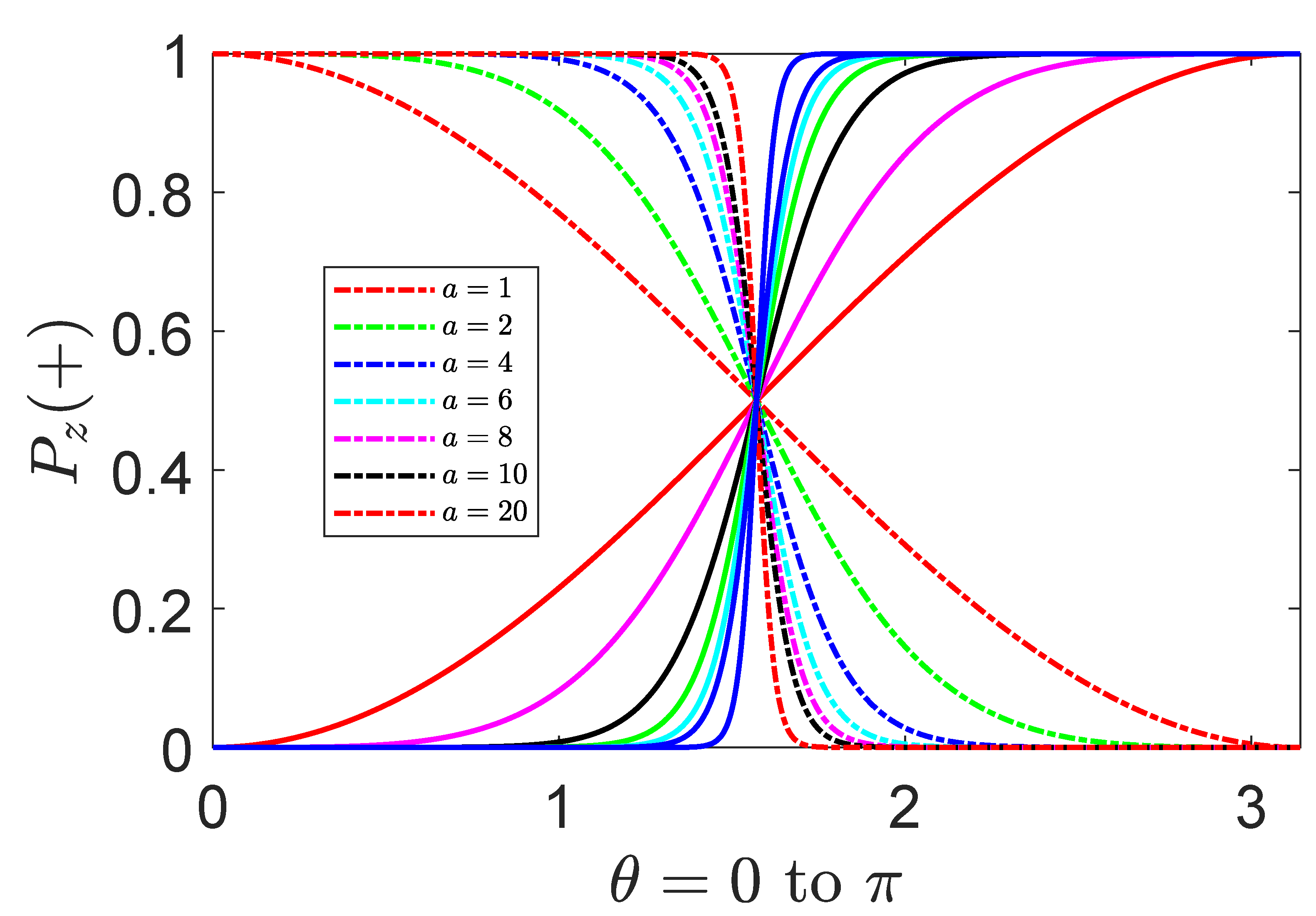
In this paper, we discuss the influences of the conformal deformation of the spherical parameters on the measurement, Berry phase, and resonance of a spin. It is shown that the physical deformations, depicted by the integer index $a=\pm n$, can be used to control the measurement of the spinor, the evolution path of the Berry phase on the Bloch sphere, and the resonant frequency. The path-tunable Berry phase is rooted in a conformal monopole that possesses the field with non-isotropic characteristic determined by the index $\pm n$. Two observations worth noticing are stated as follows:

(a) The index $\pm n$ controls the quantum-to-classical behavior of the measurement outcome of spin orientation. The spinor behaves as an ideal binary switch when the index $a=\pm n$ is large enough. Figure 8 shows the measurement of the spinor along the z direction when the index becomes $a=\pm 60$. The outcome exhibits a perfect classical switch behavior. On the other hand, at the beginning value of the index, $a=1$, the measurement exhibits an entirely stochastic property of the quantum switch. Similar correspondences can also be found in the measurements of the x and y directions. However, the classical binary property mostly appears around $\theta =\pi /2$.

Figure 8. (Color online) The spinor behaves as a classical binary switch when the index $a=\pm n$ is large enough. The graphs show the outcome in the measurement along the z direction when the index comes to $a=\pm 60$.

(b) The resonant frequency for a more general parameter surface is also given by ${\overline{\omega }}_R={\left.\sqrt{\mathrm{conformal}\mathrm{factor}}/a\right|}_n$${\omega }_R$ as (67). For instance, let us consider the resonance on the conformal ellipsoidal surface. The line element of the undeformed surface reads

$$d{s}^2=c^2({sinh}^2\eta +{sin}^2\theta )d{\theta }^2+c^2{sinh}^2\eta {sin}^2\theta d{\phi }^2,$$

(68)

where c and $\eta$ are constants that control the shape of the surface, and the ranges of the variables $0\le \theta \le \pi$, and $0\le \phi <2\pi$. Assume that the line element of the form-invariant deformation of the surface is given by

$$d{\overline{s}}^2={\overline{c}}^2({sinh}^2\overline{\eta }+{sin}^2\overline{\theta })d{\overline{\theta }}^2+{\overline{c}}^2{sinh}^2\overline{\eta }{sin}^2\overline{\theta }d{\overline{\phi }}^2,$$

(69)

where $\overline{\theta }=\overline{\theta }\left(\theta \right)$, $\overline{\phi }=\overline{\phi }\left(\phi \right)$, and $\overline{c}$ and $\overline{\eta }$ are constants. The conformal condition of the deformation is determined by

$$\frac{{\overline{c}}^2({sinh}^2\overline{\eta }+{sin}^2\overline{\theta })}{c^2({sinh}^2\eta +{sin}^2\theta )}{\left({\overline{\theta }}^{\prime }\right)}^2=\frac{{\overline{c}}^2{sinh}^2\overline{\eta }{sin}^2\overline{\theta }}{c^2{sinh}^2\eta {sin}^2\theta }{\left({\overline{\phi }}^{\prime }\right)}^2=\mathrm{conformal}\mathrm{factor}.$$

(70)

Put $\overline{\phi }=a\phi$. It can be shown that the relation between $sin\overline{\theta }$ and $sin\theta$ can be established by the Appell series $F_1$. There thus exists a conformal deformation leading to the expression (69). For our purpose of the proof of the form of ${\overline{\omega }}_R$, learning (70) is enough. Now the components of the magnetic field $\overline{\mathbf{B}}(t)=x{\widehat{e}}_x+y{\widehat{e}}_x+z{\widehat{e}}_x$ are modulated to form the conformal ellipsoidal surface

$$x=\overline{c}sinh\overline{\eta }sin\overline{\theta }cos\overline{\phi },y=\overline{c}sinh\overline{\eta }sin\overline{\theta }sin\overline{\phi },z=\overline{c}cosh\overline{\eta }cos\overline{\theta }.$$

(71)

The evolution of the spin in the field must satisfy the Schrödinger equation

$$i\hslash \frac{\partial }{\partial t}\left(\begin{array}{c}{C}_a\\ C_b\end{array}\right)=\left(\begin{array}{cc}\overline{c}cosh\overline{\eta }cos\overline{\theta }& \overline{c}sinh\overline{\eta }sin\overline{\theta }{e}^{-i\overline{\phi }}\\ \overline{c}sinh\overline{\eta }sin\overline{\theta }{e}^{i\overline{\phi }}& -\overline{c}cosh\overline{\eta }cos\overline{\theta }\end{array}\right)\left(\begin{array}{c}{C}_a\\ C_b\end{array}\right).$$

(72)

The resonant frequency has the expression

$${\overline{\omega }}_R=\frac{2\overline{c}sinh\overline{\eta }sin\overline{\theta }}{\hslash }=\frac{2\overline{c}sinh\overline{\eta }sin\overline{\theta }}{2csinh\eta sin\theta }\left(\frac{2csinh\eta sin\theta }{\hslash }\right).$$

(73)

Using (70) gives the relation

$${\overline{\omega }}_R={\left.\frac{\sqrt{\mathrm{conformal}\mathrm{factor}}}{a}\right|}_n{\omega }_R,$$

(74)

where ${\omega }_R=2csinh\eta sin\theta /\hslash$, and the conformal index taken as an integer is due to the single-valued condition about the $\phi$ variable. Obviously, a parameter surface with spherical symmetry with respect to $\phi$ would have the same conclusion.