New Comparison Results for Oscillation of Even-Order Delay Differential Equations

Abstract

In this paper, we obtain new monotonic properties for positive solutions of even-order delay differential equations in the non-canonical case. Using these properties, we establish a new oscillation criterion for solutions by comparison with an equation of the first order. The approach adopted is based on the use of symmetry between positive and negative solutions.

1. Introduction

In this work, we study the asymptotic and oscillatory behavior of positive solutions of the delay differential equation (DDE)

$${\left(a·{\vartheta }^{\left(n-1\right)}\right)}^{\prime }+\sum _{i=1}^{\kappa }{q}_i·\left(\vartheta \circ {\eta }_i\right)=0,u\ge u_0,$$

(1)

where

(H1)

$n\ge 4$ is an even natural number, $\kappa$ is a natural number, and $\left(\vartheta \circ {\eta }_i\right)\left(u\right)=\vartheta \left({\eta }_i\left(u\right)\right)$;

(H2)

$q_i\in C\left(\left[u_0,\infty \right)\right)$ and $q_i\left(u\right)\ge 0$ for $i=1,2,\dots ,\kappa ;$

(H3)

$a\in C^1\left(\left[u_0,\infty \right)\right),$$a\left(u\right)>0,$$a^{\prime }\left(u\right)\ge 0,$ and ${\int }_{u_0}^{\infty }{a}^{-1}\left(\varkappa \right)\mathrm{d}\varkappa <\infty ;$

(H4)

${\eta }_i\in C^1\left(\left[u_0,\infty \right)\right),$${\eta }_i\left(u\right)\le u,$${\eta }_i^{\prime }\left(u\right)>0$ and ${lim}_{u\to \infty }{\eta }_i\left(u\right)=\infty$ for $i=1,2,\dots ,\kappa .$

Through the solution of Equation (1), we obtain a real valued function $\vartheta \in C^{\left(n-1\right)}\left(\left[u_{\vartheta },\infty \right)\right)$, where $u_{\vartheta }⩾u_0,$ which has the property $a·{\vartheta }^{\left(n-1\right)}\in C^1\left(\left[u_{\vartheta },\infty \right)\right)$ and satisfies Equation (1) on $\left[u_{\vartheta },\infty \right)$. We consider only those solutions $\vartheta$ of Equation (1) that satisfy the following condition:

$$sup\left\{\right|\vartheta \left(u\right)|:u⩾u\}>0,\mathrm{for}u\ge u_{\vartheta }.$$

A solution of Equation (1) is called oscillatory if it has arbitrarily large zeros on $[u_{\vartheta },\infty )$; otherwise, it is said to be nonoscillatory. Equation (1) is said to be oscillatory if all of its solutions are oscillatory.

Differential equations have been and will continue to be an essential means of studying many phenomena in different sciences through modeling, analysis, and understanding these phenomena. The study of the qualitative properties of solutions to differential equations, such as oscillation, stability, symmetry, periodicity, and so on, is of great importance for understanding and studying phenomena (see, for example, [1,2,3,4]). Oscillation theory is one of the branches of the qualitative theory of differential equations which is concerned with studying the behavior of solutions without finding them. The oscillation theory sheds light on the oscillatory and nonoscillatory properties of the solution or solutions of the differential equation. A DDE is an equation for a single independent variable, usually time, in which the derivative of the dependent variable at a particular time is expressed in terms of the function’s values at earlier times.

The oscillation theory of DDEs has attracted a lot of interest, as indicated by the fact that there have been a lot of studies conducted on it. The reader is referred to the recent monographs by Agarwal et al. [5,6,7,8], Dosly and Rehák [9], Gyori and Ladas [10], and Saker [11].

Many researchers have investigated the subject of oscillation of even-order DDEs and presented many methods for finding oscillation criteria for the studied equations. In the canonical case, that is

$${\int }_{u_0}^{\infty }{a}^{-1/\alpha }\left(\varkappa \right)\mathrm{d}\varkappa =\infty ,$$

(2)

Agarwal et al. [12,13], Grace [14], Xu and Xia [15], Moaaz et al. [16], and Park et al. [17] investigated the oscillation of

$${\left(a\left(u\right){\left({\vartheta }^{\left(n-1\right)}\left(u\right)\right)}^l\right)}^{\prime }+q\left(u\right){\vartheta }^{\mathfrak{j}}\left(\eta \left(u\right)\right)=0,$$

(3)

where l and $\mathfrak{j}$ are ratios of odd integers.

In the canonical case, Equation (3) has no decreasing positive solutions, whereas in the non-canonical case, it is possible that there are decreasing positive solutions. Baculková et al. [18] investigated the asymptotic properties and oscillation of the equation

$${\left(a\left(u\right){\left({\vartheta }^{\left(n-1\right)}\left(u\right)\right)}^{\alpha }\right)}^{\prime }+q\left(u\right)f\left(\vartheta \left(\eta \left(u\right)\right)\right)=0,$$

(4)

where $f\left(\vartheta \right)$ is nondecreasing and

$$-f\left(-\vartheta y\right)\ge f\left(\vartheta y\right)\ge f\left(\vartheta \right)f\left(y\right)\mathrm{for}\vartheta y>0,$$

in both the canonical case in Equation (2) and non-canonical case; that is,

$${\int }_{u_0}^{\infty }{a}^{-1/\alpha }\left(\varkappa \right)\mathrm{d}\varkappa <\infty .$$

(5)

Furthermore, Zhang et al. [19] investigated the qualitative properties of Equation (3). They found conditions that ensured that all nonoscillatory solutions of Equation (3) converged to zero. Moaaz and Muhib [20] extended the technique used in [21] to study the oscillation by introducing a generalized Riccati substitution for Equation (3).

On the other hand, recently, Baculková [22,23] discussed the oscillatory properties of the solutions of the linear equation

$${\left(a\left(u\right){\vartheta }^{\prime }\left(u\right)\right)}^{\prime }+q\left(u\right)\vartheta \left(\eta \left(u\right)\right)=0,$$

The results in [22] extended the results of Koplatadze et al. [24] to obtain a new oscillation condition in the non-canonical case. Džurina and Jadlovská [25] proposed a one-condition oscillation criterion for the second-order delay differential equation

$${\left(a\left(u\right){\left({\vartheta }^{\prime }\left(u\right)\right)}^{\alpha }\right)}^{\prime }+q\left(u\right){\vartheta }^{\alpha }\left(\eta \left(u\right)\right)=0,$$

(6)

in the non-canonical case of Equation (5). They showed that Equation (6) is oscillatory if

$$\underset{u\to \infty }{limsup}\pi \left(u\right){\int }_{u_0}^{u}p\left(\varkappa \right)d\varkappa >1,$$

where $\pi \left(u\right):={\int }_u^{\infty }{a}^{-1}\left(\varkappa \right)d\varkappa .$

Through the latest works in the theory of oscillation, we note the development of the study of the oscillation of second-order non-canonical differential equations by obtaining new monotonical properties for the decreasing positive solutions of these equations. It is interesting to extend this development to even-order equations.

In this study, we obtain new monotonic properties for the positive solutions of Equation (1). We apply the technique used in Baculková [23] to the even-order equations of Equation (1). Then, by using an iterative technique, we improve these monotonic properties. Finally, we investigate the oscillatory behavior of the solutions to Equation (1).

Lemma 1

([26], Lemma 4). Assume that $\beta \in \left(0,1\right]$ is a ratio of odd integers. If there is a function $\rho \in C\left(\left[u_0,\infty \right),\left(0,\infty \right)\right)$ such that

$$\underset{u\to \infty }{liminf}{\int }_{{\eta }_1\left(u\right)}^u\rho \left(s\right)\mathrm{d}s>\frac{1}{\mathrm{e}},$$

then the first-order DDE $\varkappa \left(u\right)+\rho \left(u\right){\varkappa }^{\beta }\left({\eta }_1\left(u\right)\right)=0$ is oscillatory.

Lemma 2

([8], Lemma 2.2.1). Suppose that $w\in C^n\left(\left[u_0,\infty \right),\left(0,\infty \right)\right)$, and $w^{\left(n\right)}\left(u\right)$ is of a constant sign for $u\ge u_1\ge u_0$. Then, there is a nonnegative integer $\mathfrak{j}\le n$ with ${\left(-1\right)}^{n+\mathfrak{j}}{w}^{\left(n\right)}\left(u\right)\ge 0$ such that

$$\mathfrak{j}>0yields{w}^{\left(\mathfrak{j}\right)}\left(u\right)>0for\mathfrak{j}=0,1,\dots ,\mathfrak{j}-1$$

and

$$\mathfrak{j}\le n-1yields{\left(-1\right)}^{\mathfrak{j}+\mathfrak{l}}{w}^{\left(\mathfrak{l}\right)}\left(u\right)>0for\mathfrak{l}=\mathfrak{j},\mathfrak{j}+1,\dots ,n-1,$$

for $u\ge u_1$.

Theorem 1

([18], Theorem 4). All solutions of Equation (4) are oscillatory if the first-order DDEs

$$z^{\prime }\left(u\right)+q\left(u\right)f\left(\frac{{\kappa }_1{\eta }^{n-1}}{\left(n-1\right)!a^{1/\alpha }\left(\eta \left(u\right)\right)}\right)f\left(z^{1/\gamma }\left(\eta \left(u\right)\right)\right)=0,$$

$$z^{\prime }\left(u\right)+\frac{1}{a^{1/\alpha }\left(u\right)}{\left({\int }_{u_0}^{u}q\left(\varrho \right)f\left(\frac{{\kappa }_2{\eta }^{n-2}\left(\varrho \right)}{\left(n-2\right)!}\right)\mathrm{d}\varrho \right)}^{1/\gamma }{f}^{1/\gamma }\left(z\left(\eta \left(u\right)\right)\right)=0,$$

are oscillatory, and there is a $\theta \in C^1\left(\left[u_0,\infty \right)\right)$ with $\theta \left(u\right)>u$, ${\theta }^{\prime }\left(u\right)\ge 0$ and $\left({\theta }_{n-2}\circ \eta \right)\left(u\right)<u$ such that

$$z^{\prime }\left(u\right)+\frac{1}{a^{1/\alpha }\left(u\right)}{\left({\int }_{u_0}^{u}q\left(\varrho \right)\mathrm{d}\varrho \right)}^{1/\alpha }{f}^{1/\gamma }\left({\varrho }_{n-2}\left(\eta \left(u\right)\right)\right)f^{1/\gamma }\left(z\left({\theta }_{n-2}\left(\eta \left(u\right)\right)\right)\right)=0$$

is oscillatory for some ${\kappa }_1,{\kappa }_2\in \left(0,1\right)$, where

$${\theta }_1=\theta ,{\theta }_{i+1}={\theta }_i\circ \theta ,{\varrho }_1\left(u\right)=\theta -uand{\varrho }_{i+1}\left(u\right)={\int }_u^{\theta }{\varrho }_i\left(\varrho \right)\mathrm{d}\varrho ,$$

for $i=1,2,\dots ,n-3$.

2. Criteria for Nonexistence of Positive Decreasing Solution

For the sake of convenience, the symbol $\Omega$ refers to the set of all solutions of Equation (1) which eventually satisfy the property

$${\vartheta }^{\left(m\right)}\left(u\right){\vartheta }^{\left(m+1\right)}\left(u\right)<0\mathrm{for}m=0,1,2,\dots ,n-2,$$

(7)

Furthermore, we define $\eta \left(u\right):=max\left\{{\eta }_i\left(u\right),i=1,2,\dots ,n\right\}$ such that

$$a_0\left(u\right):={\int }_u^{\infty }\frac{1}{a\left(\varkappa \right)}\mathrm{d}\varkappa$$

and

$$a_m\left(u\right):={\int }_u^{\infty }{a}_{m-1}\left(\varkappa \right)\mathrm{d}\varkappa ,m=1,2,\dots ,n-2.$$

Theorem 2.

Assume that

$${\int }_{u_0}^{\infty }\frac{1}{a\left(s\right)}\left({\int }_{u_0}^s\sum _{i=1}^{\kappa }{q}_i\left(\varkappa \right)\mathrm{d}\varkappa \right)\mathrm{d}s=\infty ,$$

(8)

and there exists a ${\beta }_0\in (0,1)$ such that

$$a_{n-2}^2\left(u\right)a_{n-3}^{-1}\left(u\right)\sum _{i=1}^{\kappa }{q}_i\left(u\right)\ge {\beta }_0.$$

(9)

Therefore, if

$$\underset{u\to \infty }{liminf}{\int }_{\eta \left(u\right)}^u{a}_{n-2}\left(\varkappa \right)\left(\sum _{i=1}^{\kappa }{q}_i\left(\varkappa \right)\right)\mathrm{d}\varkappa >\frac{1-{\beta }_0}{\mathrm{e}},$$

(10)

then Ω is an empty set.

Proof. 

Assume the contrary, where $\vartheta \in \Omega$. Then, there is $u_1\ge u_0$ with $\vartheta \left(u\right)>0$ and $\vartheta \left({\eta }_i\left(u\right)\right)>0$ for all $u\ge u_1$ and $i=1,2,\dots ,\kappa$. Hence, from Equation (1), we have

$${\left(a·{\vartheta }^{\left(n-1\right)}\right)}^{\prime }=-\sum _{i=1}^{\kappa }{q}_i·\left(\vartheta \circ {\eta }_i\right).$$

(11)

Since $a{\vartheta }^{\left(n-1\right)}$ is decreasing, we obtain

$$a\left(u\right){\vartheta }^{\left(n-1\right)}\left(u\right)a_0\left(u\right)\ge {\int }_u^{\infty }\frac{a\left(\varkappa \right){\vartheta }^{\left(n-1\right)}\left(\varkappa \right)}{a\left(\varkappa \right)}\mathrm{d}\varkappa \ge -{\vartheta }^{\left(n-2\right)}\left(u\right),$$

or equivalently

$${\vartheta }^{\left(n-2\right)}\ge -a·{\vartheta }^{\left(n-1\right)}·a_0.$$

By integrating the last inequality $n-2$ times from u to $\infty ,$ and taking into account Equation (7), we arrive at

$${\left(-1\right)}^{m+1}{\vartheta }^{\left(n-m-2\right)}\le a·{\vartheta }^{\left(n-1\right)}·a_m,$$

(12)

for $m=0,1,2,\dots ,n-2$.

Since $\vartheta$ is positively decreasing, we have that ${lim}_{u\to \infty }\vartheta \left(u\right)=c\ge 0.$ Assume the contrary, where $c>0.$ Then, there is $u_2\ge u_1$ with $\vartheta \left(u\right)\ge c$ for $u\ge u_2$, and Equation (11) becomes

$${\left(a{\vartheta }^{\left(n-1\right)}\right)}^{\prime }\le -c\sum _{i=1}^{\kappa }{q}_i.$$

Whenntegrating this inequality from $u_2$ to $u,$ we get

$$a\left(u\right){\vartheta }^{\left(n-1\right)}\left(u\right)\le a\left(u_2\right){\vartheta }^{\left(n-1\right)}\left(u_2\right)-c{\int }_{u_2}^u\sum _{i=1}^{\kappa }{q}_i\left(\varkappa \right)\mathrm{d}\varkappa .$$

From Equation (7), we have $a\left(u_2\right){\vartheta }^{\left(n-1\right)}\left(u_2\right)\le 0$, and then

$${\vartheta }^{\left(n-1\right)}\left(u\right)\le -\frac{c}{a\left(u\right)}{\int }_{u_2}^u\sum _{i=1}^{\kappa }{q}_i\left(\varkappa \right)\mathrm{d}\varkappa .$$

By integrating this inequality, we find

$${\vartheta }^{\left(n-2\right)}\left(u\right)\le {\vartheta }^{\left(n-2\right)}\left(u_2\right)-c{\int }_{u_2}^u\frac{1}{a\left(\varkappa \right)}\left({\int }_{u_2}^{\varkappa }\sum _{i=1}^{\kappa }{q}_i\left(s\right)\mathrm{d}s\right)\mathrm{d}\varkappa \to -\infty \mathrm{as}u\to \infty ,$$

which contradicts with the positivity of ${\vartheta }^{\left(n-2\right)}$. Therefore,

$$\underset{u\to \infty }{lim}\vartheta \left(u\right)=0.$$

(13)

By using Equation (12) at $m=0$, we find that

$${\left(\frac{{\vartheta }^{\left(n-2\right)}}{a_0}\right)}^{\prime }=\frac{a_0·{\vartheta }^{\left(n-1\right)}+a^{-1}·{\vartheta }^{\left(n-2\right)}}{a_0^2}\ge 0,$$

which leads to

$$-{\vartheta }^{\left(n-3\right)}\left(u\right)\ge {\int }_u^{\infty }\frac{a_0\left(\varkappa \right){\vartheta }^{\left(n-2\right)}\left(\varkappa \right)}{a_0\left(\varkappa \right)}\mathrm{d}\varkappa \ge \frac{{\vartheta }^{\left(n-2\right)}\left(u\right)}{a_0\left(u\right)}{a}_1\left(u\right).$$

This implies

$${\left(\frac{{\vartheta }^{\left(n-3\right)}}{a_1}\right)}^{\prime }=\frac{a_1·{\vartheta }^{\left(n-2\right)}+a_0·{\vartheta }^{\left(n-3\right)}}{a_1^2}\le 0.$$

By repeating a similar approach $n-3$ times, we arrive at

$${\left(\frac{{\vartheta }^{\prime }}{a_{n-3}}\right)}^{\prime }\le 0\mathrm{and}{\left(\frac{\vartheta }{a_{n-2}}\right)}^{\prime }\ge 0.$$

(14)

Now, by integrating Equation (1) from $u_1$ to $u,$ and through using Equation (9), we get

$$\begin{array}{ccc}\hfill a\left(u\right){\vartheta }^{\left(n-1\right)}\left(u\right)& =& a\left(u_1\right){\vartheta }^{\left(n-1\right)}\left(u_1\right)-{\int }_{u_1}^u\sum _{i=1}^{\kappa }{q}_i\left(\varkappa \right)\vartheta \left({\eta }_i\left(\varkappa \right)\right)\mathrm{d}\varkappa \hfill \\ & \le & a\left(u_1\right){\vartheta }^{\left(n-1\right)}\left(u_1\right)-\vartheta \left(u\right){\int }_{u_1}^u\sum _{i=1}^{\kappa }{q}_i\left(\varkappa \right)\mathrm{d}\varkappa \hfill \\ & \le & a\left(u_1\right){\vartheta }^{\left(n-1\right)}\left(u_1\right)-{\beta }_0\vartheta \left(u\right){\int }_{u_1}^u\frac{a_{n-3}\left(\varkappa \right)}{a_{n-2}^2\left(\varkappa \right)}\mathrm{d}\varkappa \hfill \\ & \le & a\left(u_1\right){\vartheta }^{\left(n-1\right)}\left(u_1\right)+{\beta }_0\frac{\vartheta \left(u\right)}{a_{n-2}\left(u_2\right)}-{\beta }_0\frac{\vartheta \left(u\right)}{a_{n-2}\left(u\right)}.\hfill \end{array}$$

Since ${lim}_{u\to \infty }\vartheta \left(u\right)=0$, there is a $u_2\ge u_1$ such that $a\left(u_1\right){\vartheta }^{\left(n-1\right)}\left(u_1\right)+{\beta }_0\frac{\vartheta \left(u\right)}{a_{n-2}\left(u_2\right)}\le 0$, and so

$$a·{\vartheta }^{\left(n-1\right)}\le -{\beta }_0\frac{\vartheta }{a_{n-2}}.$$

(15)

Thus, from Equation (12) at $m=n-3$, we have

$$\frac{{\vartheta }^{\prime }}{a_{n-3}}\le -{\beta }_0\frac{\vartheta }{a_{n-2}}.$$

Consequently,

$${\left(\frac{\vartheta }{a_{n-2}^{{\beta }_0}}\right)}^{\prime }=\frac{a_{n-2}·{\vartheta }^{\prime }+{\beta }_0{a}_{n-3}·\vartheta }{a_{n-2}^{{\beta }_0+1}}\le 0.$$

(16)

Finally, we define

$$G:=a·{\vartheta }^{\left(n-1\right)}·a_{n-2}+\vartheta .$$

(17)

From Equation (12) at $m=n-2,$ we have $G\left(u\right)\ge 0$ for $u\ge u_1,$ and

$$G^{\prime }={\left(a·{\vartheta }^{\left(n-1\right)}\right)}^{\prime }·a_{n-2}-a·{\vartheta }^{\left(n-1\right)}·a_{n-3}+{\vartheta }^{\prime },$$

which, with Equation (12) at $m=n-3,$ leads to

$$G^{\prime }\le {\left(a·{\vartheta }^{\left(n-1\right)}\right)}^{\prime }·a_{n-2}=-a_{n-2}·\left(\sum _{i=1}^a{q}_i\right)\left(\vartheta \circ \eta \right).$$

(18)

By using Equations (15) and (17), we arrive at $G\le \left(1-{\beta }_0\right)\vartheta$. Thus, Equation (18) becomes

$$G^{\prime }+\frac{1}{1-{\beta }_0}{a}_{n-2}·\left(\sum _{i=1}^a{q}_i\right)\left(G\circ \eta \right)\le 0.$$

Therefore, G is a positive solution of this differential inequality. In light of Theorem 1 in [27], the associated DDE is

$$G^{\prime }+\frac{1}{1-{\beta }_0}{a}_{n-2}·\left(\sum _{i=1}^a{q}_i\right)\left(G\circ \eta \right)=0.$$

(19)

However, from Lemma 1, condition Equation (10) guarantees that Equation (19) is oscillatory. This contradiction completes the proof. □

In the following theorem, we continue to improve the monotonic properties of the positive solutions to obtain a condition that guarantees that class $\Omega$ is empty if the condition in Equation (10) is not met:

Theorem 3.

Assume that Equation (8) holds and there exists a ${\beta }_0\in (0,1)$ such that Equation (9) holds. Assume also that

$$\underset{u\to \infty }{liminf}\frac{a_{n-2}\left(\eta \left(u\right)\right)}{a_{n-2}\left(u\right)}=\lambda <\infty ,$$

(20)

and there exists an increasing sequence ${\left\{{\beta }_{\mathfrak{l}}\right\}}_{\mathfrak{l}=0}^m$ defined as

$${\beta }_{\mathfrak{l}}={\beta }_0\frac{{\lambda }^{{\beta }_{\mathfrak{l}-1}}}{1-{\beta }_{\mathfrak{l}-1}},$$

(21)

with ${\beta }_m\in \left(0,1\right)$. If

$$\underset{u\to \infty }{liminf}{\int }_{\eta \left(u\right)}^u{a}_{n-2}\left(\varkappa \right)\left(\sum _{i=1}^{\kappa }{q}_i\left(\varkappa \right)\right)\mathrm{d}\varkappa >\frac{1-{\beta }_m}{\mathrm{e}},$$

(22)

then Ω is an empty set.

Proof. 

Assume the contrary such that $\vartheta \in \Omega$. Then, there is $u_1\ge u_0$ with $\vartheta \left(u\right)>0$ and $\vartheta \left({\eta }_i\left(u\right)\right)>0$ for all $u\ge u_1$ and $i=1,2,\dots ,\kappa$. As in the proof of Theorem 2, we have that Equations (12)–(14) and (16) hold.

Since $\vartheta \left(u\right)/a_{n-2}^{{\beta }_0}\left(u\right)$ is a positive decreasing function, we see that ${lim}_{u\to \infty }\vartheta \left(u\right)/a_{n-2}^{{\beta }_0}\left(u\right)=c_1\ge 0.$ Assume the contrary, where $c_1>0.$ Then, there is a $u_2\ge u_1$ with $\vartheta \left(u\right)/a_{n-2}^{{\beta }_0}\left(u\right)\ge c_1$ for $u\ge u_2.$ Next, we define

$$W\left(u\right)=\frac{\vartheta +a·{\vartheta }^{\left(n-1\right)}·a_{n-2}}{a_{n-2}^{{\beta }_0}}.$$

Hence, from Equation (12), $W\left(u\right)\ge 0$ for $u\ge u_2.$ By differentiating $W\left(u\right)$ and using Equations (9) and (12), we find

$$\begin{array}{ccc}\hfill W^{\prime }& =& \frac{1}{a_{n-2}^{2{\beta }_0}}{a}_{n-2}^{{\beta }_0}\left({\vartheta }^{\prime }-a·{\vartheta }^{\left(n-1\right)}·a_{n-3}+{\left(a·{\vartheta }^{\left(n-1\right)}\right)}^{\prime }·a_{n-2}\right)\hfill \\ & & +{\beta }_0{a}_{n-2}^{{\beta }_0-1}·a_{n-3}·\left(\vartheta +a·{\vartheta }^{\left(n-1\right)}·a_{n-2}\right)\hfill \\ & \le & \frac{1}{a_{n-2}^{{\beta }_0+1}}\left[{\left(a·{\vartheta }^{\left(n-1\right)}\right)}^{\prime }·a_{n-2}+{\beta }_0{a}_{n-3}·\left(\vartheta +a·{\vartheta }^{\left(n-1\right)}·a_{n-2}\right)\right]\hfill \\ & \le & \frac{1}{a_{n-2}^{{\beta }_0+1}}\left[-a_{n-2}^2\sum _{i=1}^n{q}_i·\left(\vartheta \circ {\eta }_i\right)+{\beta }_0{a}_{n-3}·\left(\vartheta +a·{\vartheta }^{\left(n-1\right)}·a_{n-2}\right)\right]\hfill \\ & \le & \frac{1}{a_{n-2}^{{\beta }_0+1}}\left[-a_{n-2}^2·\vartheta \sum _{i=1}^n{q}_i+{\beta }_0{a}_{n-3}·\left(\vartheta +a·{\vartheta }^{\left(n-1\right)}·a_{n-2}\right)\right],\hfill \end{array}$$

which, with Equation (9), gives

$$W^{\prime }\le \frac{{\beta }_0}{a_{n-2}^{{\beta }_0}}{a}_{n-3}·a·{\vartheta }^{\left(n-1\right)}.$$

(23)

When using the fact that $\vartheta \left(u\right)/a_{n-2}^{{\beta }_0}\left(u\right)\ge c_1$ with Equation (15), we get

$$a·{\vartheta }^{\left(n-1\right)}\le -{\beta }_0\frac{\vartheta }{a_{n-2}}\le -{\beta }_0{c}_1{a}_{n-2}^{{\beta }_0-1}.$$

(24)

By combining Equations (23) and (24), we obtain

$$W^{\prime }\le -{\beta }_0^2{c}_1\frac{a_{n-3}}{a_{n-2}}<0.$$

By integrating the last inequality from $u_2$ to $u,$ we find

$$W\left(u_2\right)\ge {\beta }_0^2{c}_{1}ln\frac{a_{n-2}\left(u_2\right)}{a_{n-2}\left(u\right)}\to \infty \mathrm{as}u\to \infty ,$$

which is a contradiction, and so

$$\underset{u\to \infty }{lim}\frac{\vartheta \left(u\right)}{a_{n-2}^{{\beta }_0}\left(u\right)}=0.$$

(25)

Now, assume that ${\beta }_0<{\beta }_1<1$. When integrating Equation (1) from $u_1$ to u and using Equations (9), (16), and (20), we get

$$\begin{array}{ccc}\hfill a\left(u\right){\vartheta }^{\left(n-1\right)}\left(u\right)& =& a\left(u_2\right){\vartheta }^{\left(n-1\right)}\left(u_2\right)-{\int }_{u_2}^u\sum _{i=1}^{\kappa }{q}_i\left(\varkappa \right)\vartheta \left({\eta }_i\left(\varkappa \right)\right)\mathrm{d}\varkappa \hfill \\ & \le & a\left(u_2\right){\vartheta }^{\left(n-1\right)}\left(u_2\right)-\frac{\vartheta \left(u\right)}{a_{n-2}^{{\beta }_0}\left(u\right)}{\int }_{u_2}^u{a}_{n-2}^{{\beta }_0}\left(\eta \left(\varkappa \right)\right)\sum _{i=1}^{\kappa }{q}_i\left(\varkappa \right)\mathrm{d}\varkappa \hfill \\ & \le & a\left(u_2\right){\vartheta }^{\left(n-1\right)}\left(u_2\right)-\frac{\vartheta \left(u\right)}{a_{n-2}^{{\beta }_0}\left(u\right)}{\int }_{u_2}^u{\lambda }^{{\beta }_0}{a}_{n-2}^{{\beta }_0}\left(\varkappa \right)\sum _{i=1}^{\kappa }{q}_i\left(\varkappa \right)\mathrm{d}\varkappa \hfill \\ & \le & a\left(u_2\right){\vartheta }^{\left(n-1\right)}\left(u_2\right)-{\beta }_0{\lambda }^{{\beta }_0}\frac{\vartheta \left(u\right)}{a_{n-2}^{{\beta }_0}\left(u\right)}{\int }_{u_2}^u\frac{a_{n-3}\left(u\right)}{a_{n-2}^{2-{\beta }_0}\left(u\right)}\mathrm{d}\varkappa \hfill \\ & =& a\left(u_2\right){\vartheta }^{\left(n-1\right)}\left(u_2\right)+{\beta }_1\frac{\vartheta \left(u\right)}{a_{n-2}^{{\beta }_0}\left(u\right)}\frac{1}{a_{n-2}^{1-{\beta }_0}\left(u_2\right)}-{\beta }_1\frac{\vartheta \left(u\right)}{a_{n-2}\left(u\right)}.\hfill \end{array}$$

By using Equation (25), we obtain that

$$a·{\vartheta }^{\left(n-1\right)}\le -{\beta }_1\frac{\vartheta }{a_{n-2}}.$$

Consequently,

$${\left(\frac{\vartheta }{a_{n-2}^{{\beta }_1}}\right)}^{\prime }=\frac{1}{a_{n-2}^{{\beta }_1+1}}\left(a_{n-2}·{\vartheta }^{\prime }+{\beta }_1{a}_{n-3}·\vartheta \right)\le 0.$$

(26)

By repeating the same approach used previously, we can prove that ${lim}_{u\to \infty }\vartheta \left(u\right)/a_{n-2}^{{\beta }_1}\left(u\right)=0$. Similarly, if ${\beta }_{\mathfrak{j}-1}<{\beta }_{\mathfrak{j}}<1$, then we can prove that $\vartheta /a_{n-2}^{{\beta }_{\mathfrak{j}}}$ is decreasing and converges to zero, and

$$a·{\vartheta }^{\left(n-1\right)}\le -{\beta }_{\mathfrak{j}}\frac{\vartheta }{a_{n-2}},$$

(27)

for $\mathfrak{j}=2,3,\dots ,m$. Next, if we define the function G as in Equation (17) and use Equation (27) instead of Equation (15), then we get the desired result. □

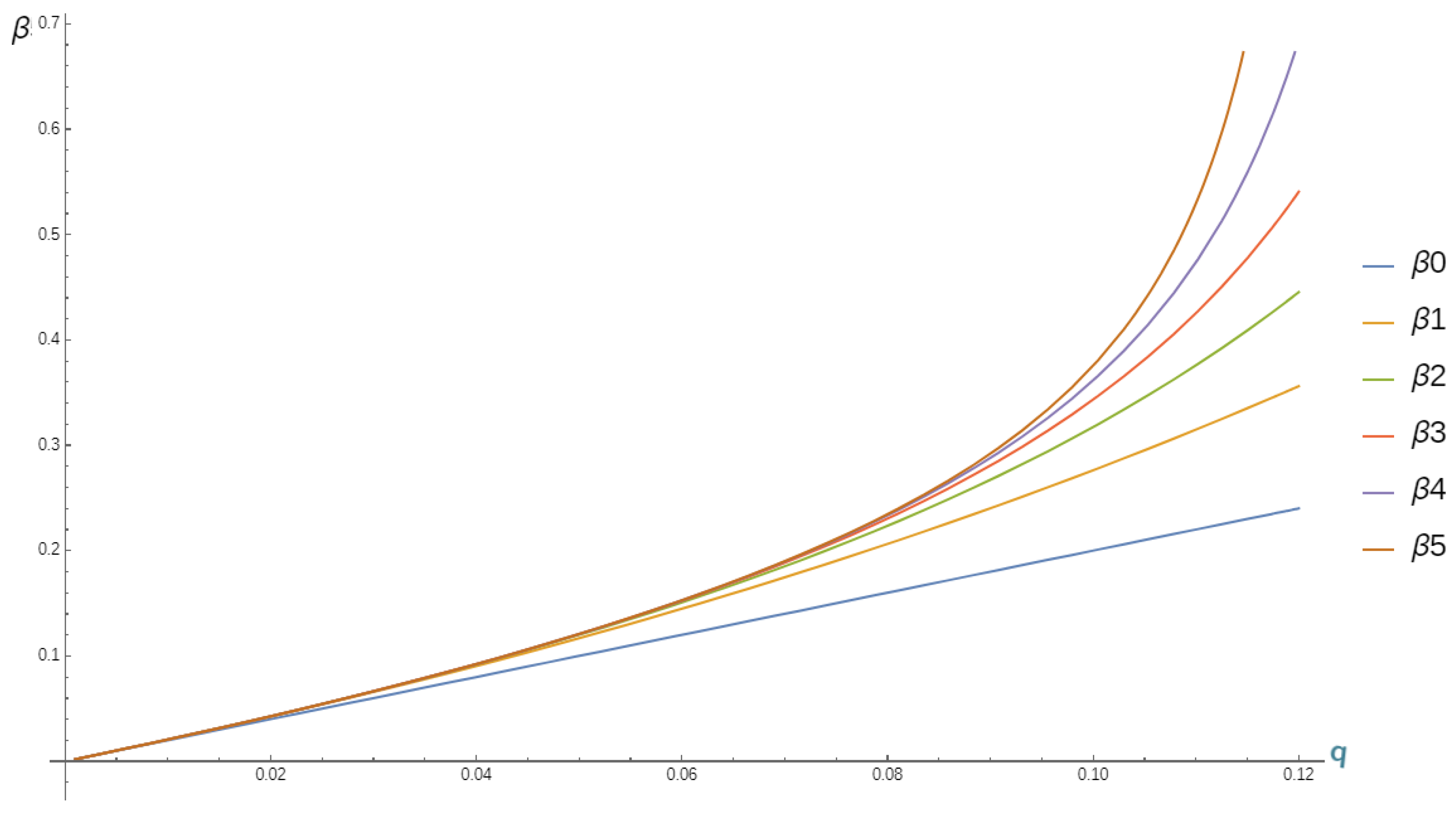
Example 1.

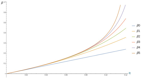
Consider the delay equation

$${\left({\mathrm{e}}^u{\vartheta }^{\left(n-1\right)}\left(u\right)\right)}^{\prime }+q_0{\mathrm{e}}^u\left(\vartheta \left(u-{\mu }_1\right)+\vartheta \left(u-{\mu }_2\right)\right)=0,u\ge 1,$$

(28)

where $q_0>0$ and $0<{\mu }_1\le {\mu }_2$. It is easy to check that $\lambda ={\mathrm{e}}^{{\mu }_1}$, $a_i\left(u\right)={\mathrm{e}}^{-u}$ for $i=0,1,2$, and the condition in Equation (8) is met. If we choose ${\beta }_0=2q_0$, then we find that Equation (9) holds. Now, we have

$${\beta }_m=\frac{{\beta }_0}{1-{\beta }_{m-1}}exp\left({\mu }_1{\beta }_{m-1}\right).$$

See Figure 1. Thus, the condition in Equation (22) reduces to

$$q_0>\frac{1-{\beta }_m}{2{\mu }_1\mathrm{e}},$$

(29)

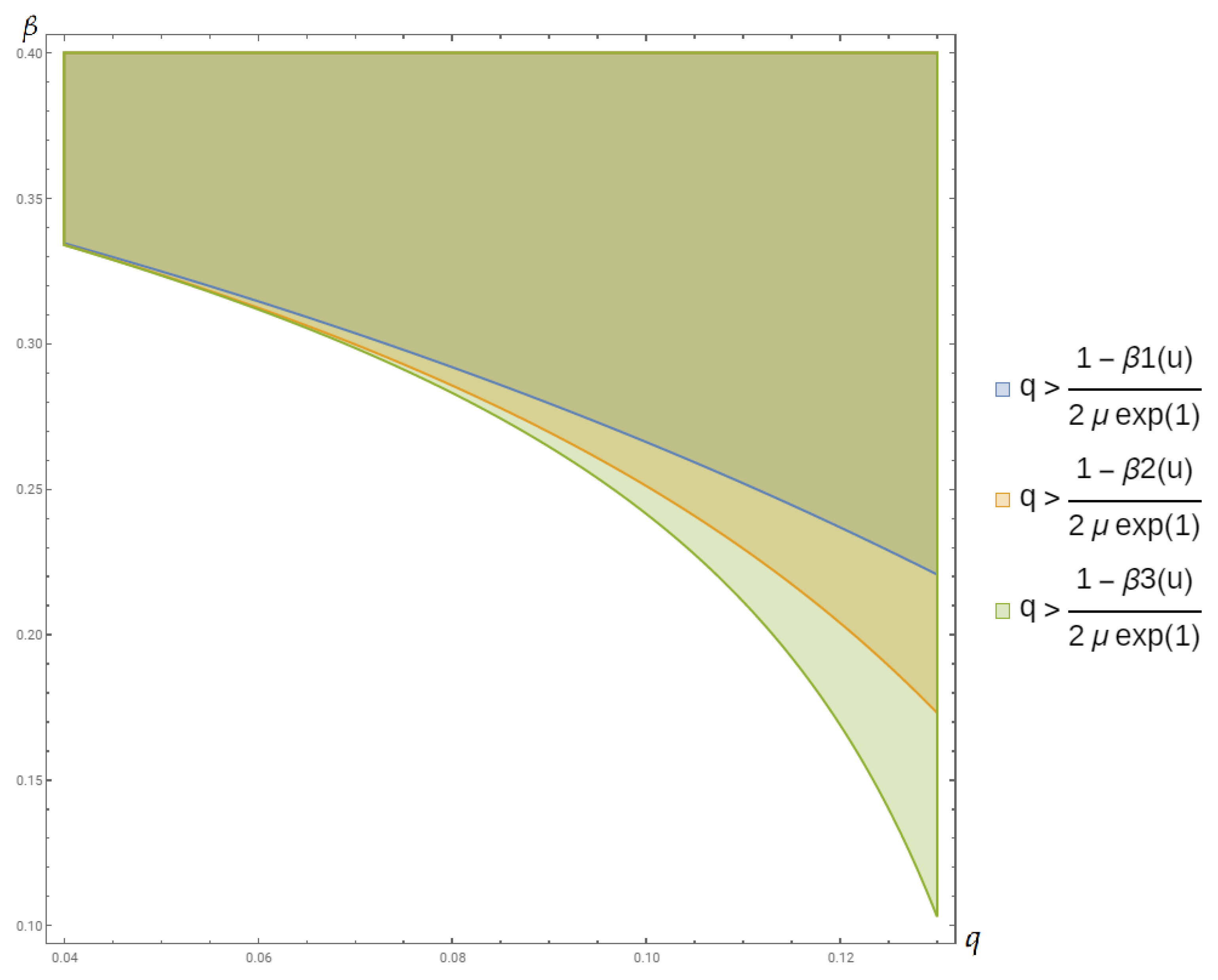
See Figure 2.

3. Oscillation Theorem

In the following, we use the results from the previous section to obtain the oscillation criteria for the solutions to Equation (1):

Theorem 4.

Let Equations (8) and (20) hold, and there exists a ${\beta }_0\in (0,1)$ such that Equation (9) holds. Let there also exist a $m\in \mathbb{N}$ such that Equation (22) holds. If

$$\underset{u\to \infty }{liminf}{\int }_{\eta \left(u\right)}^u\frac{{\eta }^{n-1}\left(\varkappa \right)}{a\left(\eta \left(\varkappa \right)\right)}\left(\sum _{i=1}^{\kappa }{q}_i\left(\varkappa \right)\right)\mathrm{d}\varkappa >\frac{\left(n-1\right)!}{\mathrm{e}}$$

and

$$\underset{u\to \infty }{liminf}{\int }_{\eta \left(u\right)}^u\frac{1}{a\left(\varkappa \right)}\left({\int }_{u_0}^{\varkappa }\left(\sum _{i=1}^{\kappa }{q}_i\left(s\right)\right){\eta }^{n-2}\left(s\right)\mathrm{d}s\right)\mathrm{d}\varkappa >\frac{\left(n-2\right)!}{\mathrm{e}},$$

then every solution to Equation (1) is oscillatory.

Proof. 

Assume the contrary, where $\vartheta$ is an eventually positive solution to Equation (1). From Lemma 2, we have the following cases:

$$\begin{array}{cc}\left(c_1\right):& {\vartheta }^{\left(\mathfrak{j}\right)}>0\mathrm{for}\mathfrak{j}=0,1,n-1\mathrm{and}{\vartheta }^{\left(n\right)}<0;\hfill \\ \left(c_2\right):& {\vartheta }^{\left(\mathfrak{j}\right)}>0\mathrm{for}\mathfrak{j}=0,1,n-2\mathrm{and}{\vartheta }^{\left(n-1\right)}<0;\hfill \\ \left(c_3\right):& {\left(-1\right)}^{\mathfrak{j}}{\vartheta }^{\left(\mathfrak{j}\right)}>0\mathrm{for}\mathfrak{j}=0,1,\dots ,n-1.\hfill \end{array}$$

It follows from Theorem 3 that $\vartheta$ does not fulfill case $\left(c_3\right)$. The proof of the case where $\left(c_1\right)$ or $\left(c_2\right)$ holds is exactly the same as the proof of Theorem 1. □

References

- Moaaz, O.; Chalishajar, D.; Bazighifan, O. Some qualitative behavior of solutions of general class of difference equations. Mathematics 2019, 7, 585. [Google Scholar] [CrossRef] [Green Version]
- Mukhin, R.R. Legacy of Alexander Mikhailovich Lyapunov and nonlinear dynamics. Appl. Nonlinear Dyn. 2018, 26, 95–120. [Google Scholar] [CrossRef]
- Myshkis, A.D. On certain problems in the theory of differential equations with deviating argument. Russ. Math. Surv. 1977, 32, 181. [Google Scholar] [CrossRef]
- Myshkis, A.D. Linear Differential Equations with Retarded Argument: Russian Book on Linear Differential Delay Equations Covering Solvability Theorems, Solution Properties, Stable and Unstable Equations, First and Second Order Equations, Periodic Equations, Etc; Izdatel’stvo Nauka: Moscow, Russia, 1972; p. 352. [Google Scholar]
- Agarwal, R.P.; Grace, S.R.; O’Regan, D. Oscillation Theory for Second Order Linear, Half-Linear, Superlinear and Sublinear Dynamic Equations; Kluwer Academic Publishers: Dordrecht, The Netherlands, 2002. [Google Scholar] [CrossRef] [Green Version]
- Agarwal, S.R.; Grace, S.R.; O’Regan, D. Oscillation Theory for Second Order Dynamic Equations; Series in Mathematical Analysis and Applications; Taylor & Francis Group: London, UK, 2003; Volume 5. [Google Scholar]
- Agarwal, R.P.; Bohner, M.; Li, W.T. Nonoscillation and Oscillation: Theory for Functional Differential Equations; Marcel Dekker, Inc.: New York, NY, USA, 2004. [Google Scholar] [CrossRef]
- Agarwal, S.R.; Grace, S.R.; O’Regan, D. Oscillation Theory for Difference and Functional Differential Equations; Kluwer Academic Publishers: Dordrecht, The Netherlands, 2000. [Google Scholar] [CrossRef]
- Došlý, O.; Rehák, P. Half-Linear Differential Equations, North-Holland Mathematics Studies; Elsevier: Amsterdam, The Netherlands, 2005; p. 202. [Google Scholar]
- Gyori, I.; Ladas, G. Oscillation Theory of Delay Differential Equations with Applications; Oxford University Press: New York, NY, USA, 1991. [Google Scholar]
- Saker, S.H. Oscillation Theory of Delay Differential and Difference Equations: Second and Third Orders; LAP Lambert Academic Publishing: Chisinau, Moldova, 2010. [Google Scholar]
- Agarwal, R.P.; Grace, S.R.; O’Regan, D. Oscillation criteria for certain nth order differential equations with deviating arguments. J. Math. Appl. Anal. 2001, 262, 601–622. [Google Scholar] [CrossRef] [Green Version]
- Agarwal, R.P.; Grace, S.R.; O’Regan, D. The oscillation of certain higher-order functional differential equations. Math. Comput. Model. 2003, 37, 705–728. [Google Scholar] [CrossRef]
- Grace, S.R. Oscillation theorems for nth-order differential equations with deviating arguments. J. Math. Appl. Anal. 1984, 101, 268–296. [Google Scholar] [CrossRef] [Green Version]
- Xu, Z.; Xia, Y. Integral averaging technique and oscillation of certain even order delay differential equations. J. Math. Appl. Anal. 2004, 292. [Google Scholar] [CrossRef]
- Moaaz, O.; Kumam, P.; Bazighifan, O. On the oscillatory behavior of a class of fourth-order nonlinear differential equation. Symmetry 2020, 12, 524. [Google Scholar] [CrossRef] [Green Version]
- Park, C.; Moaaz, O.; Bazighifan, O. Oscillation results for higher order differential equations. Axioms 2020, 9, 14. [Google Scholar] [CrossRef] [Green Version]
- Baculíková, B.; Džurina, J.; Graef, J.R. On the oscillation of higher-order delay differential equations. J. Math. Sci. 2012, 187, 387–400. [Google Scholar] [CrossRef]
- Zhang, C.; Li, T.; Suna, B.; Thandapani, E. On the oscillation of higher-order half-linear delay differential equations. Appl. Math. Lett. 2011, 24, 1618–1621. [Google Scholar] [CrossRef] [Green Version]
- Moaaz, O.; Muhib, A. New oscillation criteria for nonlinear delay differential equations of fourth-order. Appl. Math. Comput. 2020, 377, 125192. [Google Scholar] [CrossRef]
- Agarwal, R.P.; Zhang, C.; Li, T. Some remarks on oscillation of second order neutral differential equations. Appl. Math. Comput. 2016, 274, 178–181. [Google Scholar] [CrossRef]
- Baculíková, B. Oscillation of second-order nonlinear noncanonical differential equations with deviating argument. Appl. Math. Lett. 2019, 91, 68–75. [Google Scholar] [CrossRef]
- Baculíková, B. Oscillatory behavior of the second order noncanonical differential equations. Electron. J. Qual. Theory Differ. Equ. 2019, 89, 1–11. [Google Scholar] [CrossRef]
- Koplatadze, R. Criteria for the oscillation of solutions of differential inequalities and second-order equations with retarded argument. Tbiliss. Gos. Univ. Inst. Prikl. Mat. Trudy 1986, 17, 104–121. [Google Scholar]
- Dzurina, J.; Jadlovská, I. A note on oscillation of second-order delay differential equations. Appl. Math. Lett. 2017, 69, 126–132. [Google Scholar] [CrossRef]
- Baculíková, B.; Dzurina, J. Oscillation theorems for higher order neutral differential equations. Appl. Math. Comput. 2012, 219, 3769–3778. [Google Scholar] [CrossRef]
- Philos, C.G. On the existence of nonoscillatory solutions tending to zero at ∞ for differential equations with positive delays. Arch. Math. 1981, 36, 168–178. [Google Scholar] [CrossRef]
Publisher’s Note: MDPI stays neutral with regard to jurisdictional claims in published maps and institutional affiliations. |
© 2022 by the authors. Licensee MDPI, Basel, Switzerland. This article is an open access article distributed under the terms and conditions of the Creative Commons Attribution (CC BY) license (https://creativecommons.org/licenses/by/4.0/).