Monte-Carlo Simulation-Based Accessibility Analysis of Temporal Systems

Abstract

Temporal networks and network-structured systems are gaining ground in daily life. Such net-works are Vehicular Ad-hoc NETworks (VANET) and Mobile Ad-hoc NETworks (MANET), in fact, Industry 4.0 requires similar local networks. During mathematical model-based analysis of real temporal systems, it is vital to determine the existence and frequency of accessibility between components. Graph theory is a well-known mathematical tool used for studying accessibility of network components. In previous publications, the author proposed an easy-usable algorithm for determining the existence of interconnection between system-components. The Monte-Carlo Simulation can model the temporality of systems. The aim of this paper is to propose a Monte-Carlo Simulation-based method that estimates symmetry or asymmetry and the frequency of accessibilities between the components of temporal network-structured systems.

1. Introduction

Temporal networks are special network representations [1]. Their structures change depending on time. They can be applied easily for analyzing how a connected system or network develops, changes or evolves through time.

During the last years, many studies have shown applications of temporal networks in the investigation of social networks. Funel studied the causal paths structure in temporal networks of face-to-face human interactions in different social contexts [2]. Mboup et al. examined the main properties of human contact networks based on real-world data compared to artificial contact networks using synthetic mobility data [3]. Their goal was to better understand the similarities and dissimilarities between these two types of networks.

In manufacturing, Industry 4.0 technologies require local temporal networks {8}. Wersényi et al. [4] introduced the world of networked “things” as in the Industrial Internet of Things (IIoT), e.g., sensors and actuators, wearables, digital twins—by integrating distributed computation with intelligent connections.

The most often used technology for Intelligent Transportation System (ITS) is Vehicular Ad-hoc NETwork (VANET) which is a subclass of Mobile Ad-hoc NETworks (MANET). These networks enable wireless communication between vehicles as well as Road Side Units (RSUs) [5]. Boucetta and Johanyák presented a classification of different pre-existing Data Dissemination protocols in VANETs followed by the comparison and analysis of dissemination protocols from two different classes [6].

The research works of Péter et al. were directly related to the study of network traversal and can be applied to the design of vehicle dynamics [7]. For this purpose, researchers used the connection matrix of the large-scale road network model. Another research aim of theirs was to develop a laboratory model-based diagnostic procedure that performed tests of the motion processes of autonomous electric vehicles in a particular city, on a transport network or track [8].

Nagy reviewed the electronic networks used in automotive engineering, with particular reference to a fully electric vehicle [9]. The block diagram of the vehicle’s electronic network is assembled on the basis of measurements and study carried out on an electric vehicle.

Maintenance is an important technical activity that helps increase productivity, improve quality, and minimize risk and production costs. The concept of Maintenance 4.0 is referred to as a part of the fourth industrial revolution that is the current trend in automation, monitoring, and data mining for optimization of manufacturing and production processes. According to Dagdeviren, Industry 4.0 implements IIoT to increase the efficiency in manufacturing and automation where Wireless Sensor Networks (WSNs) are crucial technologies for the communication layer of IIoT [10]. The paper of Židek et al. dealt with the creation of a digital twin for an experimental assembly system based on a belt conveyor system and an automatized line for quality production check [11].

The work of Mourtzis et al. proposed an approach of machine tools and equipment maintenance, based on a monitoring system [12]. The main advantages of the proposed approach was the distribution of the real-time information, related to machine tools and cutting tools condition to the maintenance department and the operators. The real-time reporting of the machine tools failures or ageing to the maintenance experts leads to the reduction of the required maintenance time and the increase of the production rate of the shop-floor. The proposed framework utilizing the mobile technology enabled the maintenance experts to have an overview of the maintenance analysis results in a timely and efficient way and enhances their collaboration with operators.

The study of Pranowo et al. focused on the new monitoring system for the performance of maintenance works through IIoT monitored from the technician room [13]. Their work aimed to implement monitoring with easy to build and low-cost for maintenance service of production machines based on IIoT.

It is easy to see that the structures of the above-mentioned systems change randomly. Temporality of systems can be modelled by Monte-Carlo Simulation (MCS) [14].

The MCS is one of generally usable simulation techniques related to the use of random numbers. The publication of Metropolis and Ulam offered a general description of a method dealing with a class of problems in mathematical physics [15]. They were the first to name this method “Monte-Carlo”.

The present paper focuses on the methodology of Monte-Carlo Simulation-based investigation of symmetry or asymmetry of temporal systems and determination of their accessibilities.

It is organized as follows: It starts with presenting the core model of the proposed method in Section 2. Section 3 describes the methodology of structural analysis. Section 4 shows the functional analysis. Finally, Section 5 concludes this paper, summarizes the main findings of this research and offers some future research directions.

2. The Core Method

As a first step, for the model of accessibility matrix determination of the given system should be determined if its graph is a so-called simple—not temporal—one (all edges work steadily).

When investigating the accessibility of a graph that depicts the structure (connections between elements) of a system it is important to determine its adjacency matrix. The adjacency matrix A of a directed graph shows the links directly connecting node p_i to node p_j [16,17]:

$$a_{ij}=\{\begin{array}{cc}1& \mathrm{there}\mathrm{is}\mathrm{a}\mathrm{directed}\mathrm{edge}\mathrm{from}{p}_i\mathrm{to}{p}_j\\ 0& \mathrm{otherwise}\end{array},$$

(1)

If there are not self-loop in the graph, the elements of main diagonal should be zero.

The directed graph shown in Figure 1 has the following adjacent matrix:

$$A=\left[\begin{array}{ccccccccccccccc}0& 0& 0& 1& 0& 0& 0& 0& 0& 0& 0& 0& 0& 0& 0\\ 1& 0& 0& 0& 0& 0& 0& 0& 0& 0& 0& 0& 0& 0& 0\\ 0& 0& 0& 1& 0& 0& 0& 0& 0& 0& 0& 0& 0& 0& 0\\ 0& 0& 0& 0& 0& 1& 0& 0& 0& 0& 0& 0& 0& 0& 0\\ 0& 0& 0& 0& 0& 0& 1& 0& 1& 0& 1& 0& 0& 0& 0\\ 0& 0& 0& 0& 1& 0& 0& 0& 0& 0& 0& 0& 0& 1& 0\\ 0& 0& 0& 0& 0& 0& 0& 0& 0& 0& 0& 0& 0& 0& 0\\ 0& 1& 0& 0& 0& 0& 0& 0& 0& 0& 0& 0& 0& 0& 0\\ 0& 0& 0& 0& 0& 0& 0& 1& 0& 0& 0& 0& 0& 0& 0\\ 0& 1& 0& 0& 0& 0& 0& 0& 0& 0& 0& 0& 0& 0& 0\\ 0& 1& 0& 0& 0& 0& 0& 0& 0& 0& 0& 0& 0& 0& 0\\ 0& 0& 1& 0& 0& 0& 0& 0& 0& 0& 0& 0& 0& 0& 0\\ 0& 0& 1& 0& 0& 0& 0& 0& 0& 0& 0& 0& 0& 0& 0\\ 0& 0& 1& 0& 0& 0& 0& 0& 0& 0& 0& 0& 0& 0& 0\\ 0& 0& 1& 0& 0& 0& 0& 0& 0& 0& 0& 0& 0& 0& 0\end{array}\right],$$

(2)

The elements of the matrix Aⁿ are the number of paths of length n connecting the nodes. Funel [4] introduced the binary operator $ƛ$, which acts on general parameter η in the following way:

$$ƛ\left(\eta \right)=\{\begin{array}{ccc}1& \mathrm{if}& \eta \ne 0\\ 0& \mathrm{if}& \eta =0\end{array},$$

(3)

while the accessibility matrix can be determined by the equation

$$Z=ƛ\left({\displaystyle \sum _{i=1}^m{A}^i}\right),$$

(4)

where m is the number of nodes.

Funel’s method is generally easy to use, but in the case of many nodes and edges, the calculation has a very long run. To overcome this shortcoming, in an earlier publication [4] the author proposed a different method, taking into account the following conditions:

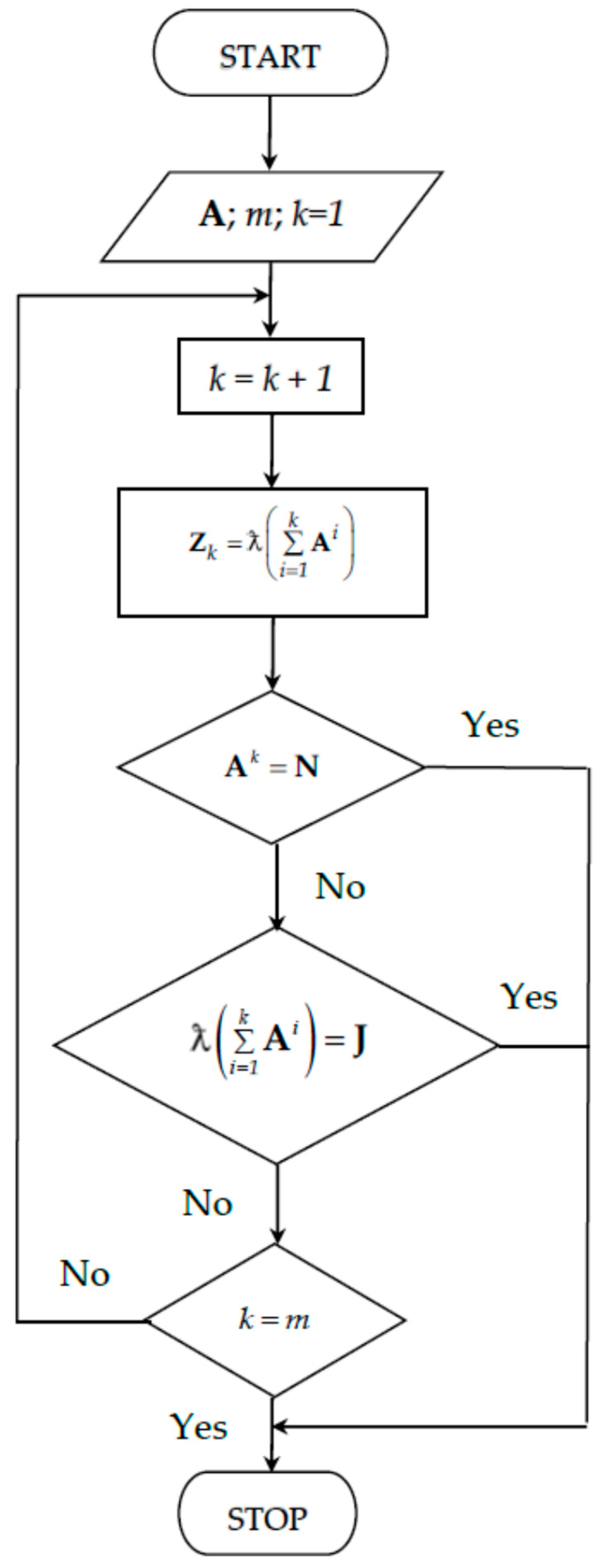
• If there exists k such that

  $$A^k=N,$$

  (5)

  where N is zero (null) matrix, then the length of the longest path of graph is k − 1; so further calculation is unnecessary.
• If

  $$ƛ\left({\displaystyle \sum _{i=1}^k{A}^i}\right)=J,$$

  (6)

  where J is matrix of ones, then all nodes have connection with all other ones; so further calculation is unnecessary too.

Figure 2 presents the block diagram of accessibility matrix determination.

The accessibility matrix shows the interconnection between nodes. But, through the investigation of the accessibility matrix, the impacts and exposures of nodes (systems elements) can be characterized too.

The impact vector

$$\begin{array}{cc}i=\left[i_k\right]& i_k={\displaystyle \sum _{j=1}^m{z}_{kj}}\end{array},$$

(7)

represents which node(s) has/have the highest effect on the other ones.

From an engineering point of view the system elements can be of different importance, which is characterized by their weight values and

$$w^T=\left[\begin{array}{cccc}{w}_1& w_2& \dots & w_m\end{array}\right],$$

(8)

weight vector of given system (graph). The weighted impact vector can be determined by using the equation

$$\begin{array}{cc}{i}_W=i\odot w& i_{wk}=i_k{w}_k\end{array},$$

(9)

where the operator ⊙ denotes the element-wise multiplication.

The normalized (sum of weights are one) weight vector of directed graph given in Figure 1:

$$w^T=\left[\begin{array}{ccccccccccccccc}0.04& 0.07& 0.10& 0.06& 0.06& 0.06& 0& 0.05& 0.05& 0.21& 0.05& 0.07& 0.07& 0.04& 0.076\end{array}\right]$$

(10)

The exposure vector

$$\begin{array}{cc}e=\left[e_k\right]& e_k={\displaystyle \sum _{j=1}^m{z}_{jk}}\end{array},$$

(11)

shows the exposedness of nodes, i.e., which node (system element) depends the most on the other ones.

Applying the above mentioned method—Equations (2)–(11)—the investigated simple graph has the following accessibility matrix:

$$Z=\left[\begin{array}{ccccccccccccccc}1& 1& 1& 1& 1& 1& 1& 1& 1& 0& 1& 0& 0& 1& 0\\ 1& 1& 1& 1& 1& 1& 1& 1& 1& 0& 1& 0& 0& 1& 0\\ 1& 1& 1& 1& 1& 1& 1& 1& 1& 0& 1& 0& 0& 1& 0\\ 1& 1& 1& 1& 1& 1& 1& 1& 1& 0& 1& 0& 0& 1& 0\\ 1& 1& 1& 1& 1& 1& 1& 1& 1& 0& 1& 0& 0& 1& 0\\ 1& 1& 1& 1& 1& 1& 1& 1& 1& 0& 1& 0& 0& 1& 0\\ 0& 0& 0& 0& 0& 0& 0& 0& 0& 0& 0& 0& 0& 0& 0\\ 1& 1& 1& 1& 1& 1& 1& 1& 1& 0& 1& 0& 0& 1& 0\\ 1& 1& 1& 1& 1& 1& 1& 1& 1& 0& 1& 0& 0& 1& 0\\ 1& 1& 1& 1& 1& 1& 1& 1& 1& 0& 1& 0& 0& 1& 0\\ 1& 1& 1& 1& 1& 1& 1& 1& 1& 0& 1& 0& 0& 1& 0\\ 1& 1& 1& 1& 1& 1& 1& 1& 1& 0& 1& 0& 0& 1& 0\\ 1& 1& 1& 1& 1& 1& 1& 1& 1& 0& 1& 0& 0& 1& 0\\ 1& 1& 1& 1& 1& 1& 1& 1& 1& 0& 1& 0& 0& 1& 0\\ 1& 1& 1& 1& 1& 1& 1& 1& 1& 0& 1& 0& 0& 1& 0\end{array}\right],$$

(12)

impact vector:

$$i^T=\left[\begin{array}{ccccccccccccccc}11& 11& 11& 11& 11& 11& 0& 11& 11& 11& 11& 11& 11& 11& 11\end{array}\right],$$

(13)

weighted impact vector:

$$i_w^T=\left[\begin{array}{ccccccccccccccc}0.38& 0.76& 1.14& 0.62& 0.70& 0.62& 0& 0.57& 0.54& 2.29& 0.57& 0.76& 0.76& 0.46& 0.84\end{array}\right],$$

(14)

and exposure vector:

$$e^{\mathcal{T}}=\left[\begin{array}{ccccccccccccccc}14& 14& 14& 14& 14& 14& 14& 14& 14& 0& 14& 0& 0& 14& 0\end{array}\right],$$

(15)

The above results highlight only the facts of possible accessibilities and their consequences. The real temporal system adjacencies can change randomly, so this suddenness should be modelled by MCS.

3. Structural Analysis

In the case of temporal system, the connections between elements are uncertain, change randomly over time. In the case of VANETs these uncertainties occurr by the vehicles’ moving, when they change their connections with RSUs. For example, in the IIoT nodes 12; 13 and 15 can be same type machine-tools, which are used—so they connect with edge 3—depending on the momentary production requirements. These uncertainties can be modelled by MCS. Connections between elements of temporal systems can be depicted by weighted directed graphs, in which weights of edges are the probability that the directed edge is working.

During MCS, in the beginning, random numbers are generated in the interval [0; 1] follow uniform distribution. Then the temporary connections between the elements of the graph describing the system are determined as a function of the weights, existence probability, assigned to the possible directed edge and given random number:

$$a_{ijs}=\{\begin{array}{cc}1& {\mathrm{if}\mathrm{w}}_k<r_{se}\\ 0& \mathrm{otherwise}\end{array},$$

(16)

where w_k is weight of kth edge and r_se is the random number generated for the eth (from p_i to p_j) edge in the case of the sth excitation.

Knowing the momentary adjacent matrices, the momentary accessibility matrices, the impact and exposure vectors can be determined—using the core method.

After all excitations, the average availability matrix

$$Z_Q=\frac{{\displaystyle \sum _{k=1}^Q{Z}_k}}{Q},$$

(17)

average impact vector

$$i_Q=\frac{{\displaystyle \sum _{k=1}^Q{i}_k}}{Q},$$

(18)

average exposure

$$e_Q=\frac{{\displaystyle \sum _{k=1}^Q{e}_k}}{Q},$$

(19)

and weighted average impact vector

$$i_{wQ}=i_Q\odot w,$$

(20)

can be calculated, where Q is number of excitation (number of model runs with different input data).

To investigate accessibilities of temporal system from structural point of view, the author investigated the graph illustrated in Figure 1, assuming that the weights of all edges are 0.8. Then, in the case of excitation number 1,000,000 (1M), the average accessibility matrix is:

$$Z_{1M}=\left[\begin{array}{ccccccccccccccc}0.34& 0.42& 0.41& 0.80& 0.51& 0.64& 0.41& 0.33& 0.41& 0& 0.41& 0& 0& 0.51& 0\\ 0.80& 0.34& 0.33& 0.64& 0.41& 0.51& 0.33& 0.26& 0.33& 0& 0.33& 0& 0& 0.41& 0\\ 0.34& 0.42& 0.41& 0.80& 0.51& 0.64& 0.41& 0.33& 0.41& 0& 0.41& 0& 0& 0.51& 0\\ 0.42& 0.53& 0.51& 0.57& 0.64& 0.80& 0.51& 0.41& 0.51& 0& 0.51& 0& 0& 0.64& 0\\ 0.66& 0.82& 0.27& 0.53& 0.34& 0.42& 0.80& 0.64& 0.80& 0& 0.8& 0& 0& 0.34& 0\\ 0.53& 0.66& 0.64& 0.72& 0.8& 0.57& 0.64& 0.51& 0.64& 0& 0.64& 0& 0& 0.8& 0\\ 0& 0& 0& 0& 0& 0& 0& 0& 0& 0& 0& 0& 0& 0& 0\\ 0.64& 0.8& 0.26& 0.51& 0.33& 0.41& 0.26& 0.21& 0.26& 0& 0.26& 0& 0& 0.33& 0\\ 0.51& 0.64& 0.21& 0.41& 0.26& 0.33& 0.21& 0.80& 0.21& 0& 0.21& 0& 0& 0.26& 0\\ 0.64& 0.80& 0.26& 0.51& 0.33& 0.41& 0.26& 0.21& 0.26& 0& 0.26& 0& 0& 0.33& 0\\ 0.64& 0.80& 0.26& 0.51& 0.33& 0.41& 0.26& 0.21& 0.26& 0& 0.26& 0& 0& 0.33& 0\\ 0.27& 0.34& 0.80& 0.64& 0.41& 0.51& 0.33& 0.26& 0.33& 0& 0.33& 0& 0& 0.41& 0\\ 0.27& 0.34& 0.80& 0.64& 0.41& 0.51& 0.33& 0.26& 0.33& 0& 0.33& 0& 0& 0.41& 0\\ 0.27& 0.34& 0.80& 0.64& 0.41& 0.51& 0.33& 0.26& 0.33& 0& 0.33& 0& 0& 0.41& 0\\ 0.27& 0.34& 0.80& 0.64& 0.41& 0.51& 0.33& 0.26& 0.33& 0& 0.327& 0& 0& 0.41& 0\end{array}\right]$$

(21)

average impact vector:

$$i_{1M}^T=\left[\begin{array}{ccccccccccccccc}5.19& 4.68& 5.18& 6.06& 6.41& 7.15& 0& 4.27& 4.05& 4.27& 4.28& 4.62& 4.63& 4.62& 4.64\end{array}\right]$$

(22)

weighted average impact vector:

$$i_{w1M}^T=\left[\begin{array}{ccccccccccccccc}0.18& 0.33& 0.54& 0.34& 0.4& 0.4& 0& 0.22& 0.2& 0.89& 0.22& 0.32& 0.32& 0.19& 0.35\end{array}\right]$$

(23)

average exposure vector:

$$e_{1M}^T=\left[\begin{array}{ccccccccccccccc}6.59& 7.58& 6.76& 8.56& 6.09& 7.18& 5.40& 4.95& 5.40& 0& 5.40& 0& 0& 6.09& 0\end{array}\right]$$

(24)

The comparison of vectors Equations (22) and (23) (illustrated by the graphs of Figure 3) highlights that taking into account the weight (importance within the system) of nodes (elements) gives a significantly different result from the structural impacts.

4. Functional Analysis

To analyze accessibilities of temporal system from functional point of view, the author investigated the weighted directed graph illustrated in Figure 4.

Then, in the case of excitation number 1,000,000 (1M), the average accessibility matrix is:

$$Z_{1M}=\left[\begin{array}{ccccccccccccccc}0.35& 0.43& 0.37& 0.80& 0.61& 0.68& 0.61& 0.37& 0.46& 0& 0.43& 0& 0& 0,41& 0\\ 0.82& 0.35& 0.30& 0.66& 0.50& 0.56& 0.50& 0.30& 0.38& 0& 0.35& 0& 0& 0.33& 0\\ 0.37& 0.45& 0.39& 0.85& 0.65& 0.72& 0.64& 0.39& 0.49& 0& 0.46& 0& 0& 0.43& 0\\ 0.44& 0.53& 0.46& 0.58& 0.77& 0.85& 0.76& 0.46& 0.57& 0& 0.54& 0& 0& 0.51& 0\\ 0.57& 0.70& 0.21& 0.46& 0.35& 0.39& 0.99& 0.60& 0.75& 0& 0.70& 0& 0& 0.23& 0\\ 0.52& 0.63& 0.54& 0.68& 0.90& 0.58& 0.89& 0.54& 0.68& 0& 0.63& 0& 0& 0.60& 0\\ 0& 0& 0& 0& 0& 0& 0& 0& 0& 0& 0& 0& 0& 0& 0\\ 0.66& 0.80& 0.24& 0.52& 0.40& 0.45& 0.40& 0.24& 0.30& 0& 0.28& 0& 0& 0.27& 0\\ 0.52& 0.64& 0.19& 0.42& 0.32& 0.36& 0.32& 0.80& 0.24& 0& 0.22& 0& 0& 0.21& 0\\ 0.81& 0.99& 0.30& 0.65& 0.50& 0.55& 0.49& 0.30& 0.37& 0& 0.35& 0& 0& 0.33& 0\\ 0.49& 0.60& 0.18& 0.39& 0.30& 0.33& 0.30& 0.18& 0.23& 0& 0.21& 0& 0& 0.20& 0\\ 0.36& 0.45& 0.98& 0.83& 0.64& 0.71& 0.63& 0.38& 0.48& 0& 0.45& 0& 0& 0.42& 0\\ 0.26& 0.32& 0.70& 0.60& 0.46& 0.51& 0.45& 0.27& 0.34& 0& 0.32& 0& 0& 0.30& 0\\ 0.33& 0.41& 0.90& 0.76& 0.59& 0.65& 0.58& 0.35& 0.44& 0& 0.41& 0& 0& 0.39& 0\\ 0.32& 0.39& 0.85& 0.72& 0.55& 0.61& 0.55& 0.33& 0.41& 0& 0.39& 0& 0& 0.37& 0\end{array}\right]$$

(25)

average impact vector:

$$i_{1M}^T=\left[\begin{array}{ccccccccccccccc}5.5& 5.04& 5.85& 6.46& 5.95& 7.18& 0& 4.56& 4.25& 5.63& 3.41& 6.33& 4.52& 5.81& 5.49\end{array}\right]$$

(26)

weighted average impact vector:

$$i_{w1M}^T=\left[\begin{array}{ccccccccccccccc}0.19& 0.35& 0.61& 0.36& 0.37& 0.4& 0& 0.24& 0.21& 1.17& 0.18& 0.44& 0.31& 0.24& 0.42\end{array}\right]$$

(27)

average exposure vector:

$$e_{1M}^T=\left[\begin{array}{ccccccccccccccc}6.82& 7.68& 6.6& 8.93& 7.53& 7.94& 8.1& 5.52& 6.13& 0& 5.73& 0& 0& 5.01& 0\end{array}\right],$$

(28)

The Figure 5 shows results of Functional Analysis.

5. Conclusions

In this paper, an easy-to-use MCS-based algorithm for investigation of accessibilities of temporary systems was presented. The proposed method can be used to determine the existence and consequences of accessibilities between system components.

The following conclusions can be drawn from Cora Method—Section 2:

(2.a)

the exposure vector e illustrates that the components 10; 12; 13 and 15 are not affected by a dysfunction of an-other system element;

(2.b)

the impact vector i shows that failures of component 7 has no effect on the work of the other system elements;

(2.c)

application of the weighted impact vector provides that element 15 has the most weighted effect on the work of other system elements;

The following conclusions can be drawn from the results of the structural investigation—Section 3:

(3.a)

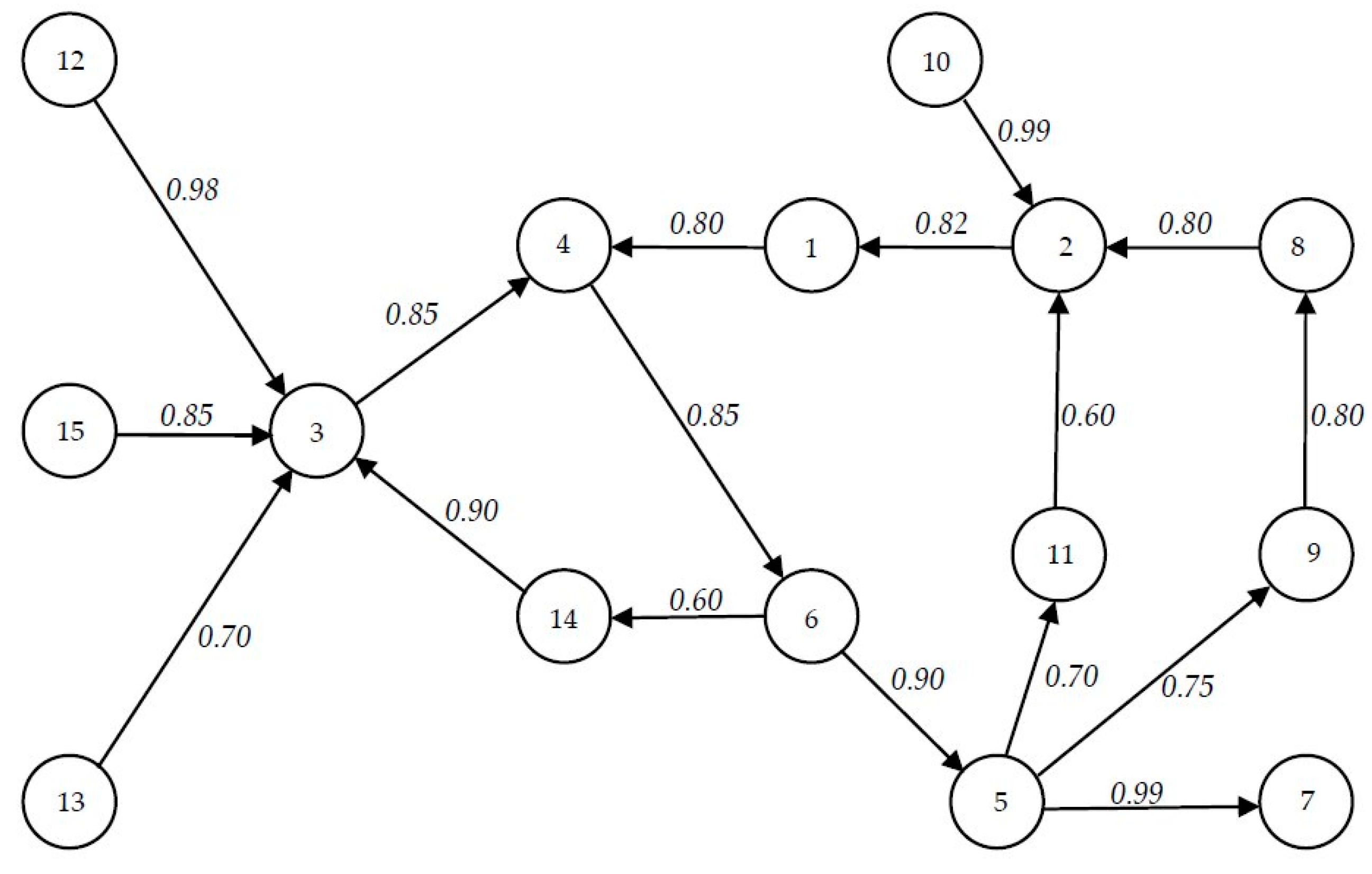
the maximum accessibility is from element 5 to element 2 (z_5.2 = 0.82);

(3.b)

the minimal, but not zero, (0.21) accessibility is from element 9 to elements 3, 7, 9 and 11;

(3.c)

the average impact vector i_1M shows that failure of component 6 has the maximum effect on the work of the other system elements (i_6.1M = 7.15);

(3.d)

element 9 has the minimal, but not zero, impact on the other nodes;

(3.e)

element 10 has the highest weighted average impact;

(3.f)

element has smallest, but not zero, weighted average impact;

(3.g)

components 10; 12; 13 and 15 are not affected by a dysfunction of another system element—compare with conclusion 2.a).

(3.h)

element 8 has the minimum, but not zero, exposure.

It follows from the conclusions above that, due to the uncertain adjacencies between the temporal graph nodes (temporal system elements), the accessibilities, impacts and exposures are significantly different within the graph (system). This can be clearly seen by comparing the matrices (12) and (21), vectors (13) and (22), and vectors (15) and (24). Based on the results obtained using the same edge weights (existence probabilities of adjacencies) and element weights importance of elements), the following definitions are suggested to introduce:

• structural accessibility;
• structural impact;
• structural exposure.

These system characteristics are only determined by the locations within the graph (system) and the relationships between the nodes (elements).

The following conclusions can be drawn from results of the functional investigation—Section 4:

(4.a)

the maximum average accessibility is from element 5 to element 7 (z_5.7 = 0.99);

(4.b)

the minimal, but not zero, (0.21) average accessibilities are from element 1 to element 8;

(4.c)

component 6 has the maximum average effect on the work of the other system elements (i_6.1M = 7.18);

(4.d)

element 11 has a minimal, but not zero, average impact on other nodes;

(4.e)

element 10 has the highest weighted average impact;

(4.f)

element 11 has smallest, but not zero, weighted average impact;

(4.g)

the element 14 has the minimum, but not zero, average exposure;

(4.h)

element 4 has the maximum average exposure.

It is worth paying extra attention to the impact values of elements 12; 13 and 15. In the case of the structural analysis, they have almost identical values (4.62; 4.63 and 4.64), as they occupy a similar place in the structure of the system. But, during the functional analysis, they have significantly different impact values (6.33; 4.52 and 5.49) due to the different weights of the edges directed to element 3, i.e., their different functional tasks (momentary production requirements) in the system.

Based on the difference between the results of structural and functional analysis, the author proposes the introduction of the following definitions:

• functional accessibility;
• functional impact;
• functional exposure.

These characteristics are determined not only by the location and relationship of the given element within the system, but also by its functional role.

The drawback of the proposed method is that its elapsed time increases significantly if the number of nodes, edges and excitations increases. Figure 6 demonstrates that the elapsed time of MCS depends on the number of excitations.

The Author’s prospective future research direction is the study of methodologies of interconnections and reliability of systems with complex interconnections.

References

- Lentz, H.; Selhorst, T.; Sokolov, M. Unfolding Accessibility Provides a Macroscopic Approach to Temporal Networks. Phys. Rev. Lett. 2013, 25, 788–795. [Google Scholar] [CrossRef] [PubMed]
- Funel, A. Causal Paths in Temporal Networks of Face-to-Face Human Interactions. Complex Syst. 2021, 30, 33–46. [Google Scholar] [CrossRef]
- Mboup, D.; Diallo, C.; Cherifi, H. Temporal Networks Based on Human Mobility Models: A Comparative Analysis With Real-World Networks. IEEE Access 2022, 10, 5912–5935. [Google Scholar] [CrossRef]
- Wersényi, G.; Csapó, Á.; Budai, T.; Baranyi, P. Internet of Digital Reality: Infrastructural Background—Part II. Acta Polytech. Hung. 2021, 18, 91–104. [Google Scholar] [CrossRef]
- Boucetta, S.I.; Guichi, Y.; Johanyák, Z.C. Simulation-Based Comparison and Analysis of Time-Based and Topology-Based Emergency Dissemination Protocols in Vehicular Ad-hoc NETworks. In Proceedings of the 6th International Conference on Systems and Informatics (ICSAI 2019), Shanghai, China, 2–4 November 2019. [Google Scholar]
- Boucetta, S.I.; Johanyák, Z.C. Review of Mobility Scenarios Generators for Vehicular Ad-Hoc Networks Simulators. J. Phys. Conf. Ser. 2021, 1935, 012006. [Google Scholar] [CrossRef]
- Péter, T.; Háry, A.; Szauter, F.; Szabó, K.; Vadvári, T.; Lakatos, I. Analysis of Network Traversal and Qualification of the Testing Values of Trajectories. Acta Polytech. Hung. 2021, 18, 151–161. [Google Scholar] [CrossRef]
- Péter, T.; Szauter, F.; Rózsás, Z.; Lakatos, I. Integrated application of network traffic and intelligent driver models in the test laboratory analysis of autonomous vehicles and electric vehicles. Int. J. Heavy Veh. Syst. 2020, 27, 227–245. [Google Scholar] [CrossRef]
- Nagy, I. Hierarchical Mapping of an Electric Vehicle Sensor and Control Network. Acta Polytech. Hung. 2021, 18, 161–180. [Google Scholar] [CrossRef]
- Dagdeviren, Z.A. Weighted Connected Vertex Cover Based Energy-Efficient Link Monitoring for Wireless Sensor Networks Towards, Secure Internet of Things. IEEE Access 2021, 9, 10107–10119. [Google Scholar] [CrossRef]
- Židek, K.; Pitel’, J.; Adámek, M.; Lazorík, P.; Hošovský, A. Digital Twin of Experimental Smart Manufacturing Assembly System for Industry 4.0 Concept. Sustainability 2020, 12, 3658. [Google Scholar] [CrossRef]
- Mourtzis, D.; Vlachou, E.; Milas, N.; Xanthopoulos, N. A Cloud-based Approach for Maintenance of Machine Tools and Equipment Based on Shop-floor Monitoring. Procedia CIRP 2016, 41, 655–660. [Google Scholar] [CrossRef] [Green Version]
- Pranowo, I.D.; Artanto, D. Smart monitoring system using NodeMCU for maintenance of production machines. Indones. J. Elec. Eng. Comp. Sci. 2022, 25, 788–795. [Google Scholar] [CrossRef]
- Pokorádi, L. Availability assessment with Monte-Carlo simulation of maintenance process model. Polytech. Univ. Buchar. Sci. Bull. Ser. D Mech. Eng. 2016, 78, 43–54. [Google Scholar]
- Metropolis, N.; Ulam, S. The Monte Carlo Method. J. Am. Stat. Assoc. 1949, 44, 335–341. [Google Scholar] [CrossRef]
- Pokorádi, L. Graph model-based analysis of technical systems. IOP Conf. Ser. Mater. Sci. Eng. 2018, 393, 012007. [Google Scholar] [CrossRef]
- Pokorádi, L. Methodology of Advanced Graph Model-based Vehicle Systems’ Analysis. In Proceedings of the IEEE 18th International Symposium on Computational Intelligence and Informatics (CINTI 2018), Budapest, Hungary, 20–22 November 2018. [Google Scholar]
Publisher’s Note: MDPI stays neutral with regard to jurisdictional claims in published maps and institutional affiliations. |
© 2022 by the author. Licensee MDPI, Basel, Switzerland. This article is an open access article distributed under the terms and conditions of the Creative Commons Attribution (CC BY) license (https://creativecommons.org/licenses/by/4.0/).
Share and Cite
Pokorádi, L. Monte-Carlo Simulation-Based Accessibility Analysis of Temporal Systems. Symmetry 2022, 14, 983. https://doi.org/10.3390/sym14050983
Pokorádi L. Monte-Carlo Simulation-Based Accessibility Analysis of Temporal Systems. Symmetry. 2022; 14(5):983. https://doi.org/10.3390/sym14050983
Chicago/Turabian StylePokorádi, László. 2022. "Monte-Carlo Simulation-Based Accessibility Analysis of Temporal Systems" Symmetry 14, no. 5: 983. https://doi.org/10.3390/sym14050983
APA StylePokorádi, L. (2022). Monte-Carlo Simulation-Based Accessibility Analysis of Temporal Systems. Symmetry, 14(5), 983. https://doi.org/10.3390/sym14050983