
Viable Requirements of Curvature Coupling Helical Magnetogenesis Scenario


Department of Physics, Chandernagore College, Hooghly 712 136, India
Symmetry 2022, 14(6), 1086; https://doi.org/10.3390/sym14061086
Submission received: 23 April 2022
/
Revised: 13 May 2022
/
Accepted: 20 May 2022
/
Published: 25 May 2022
(This article belongs to the Section Physics)
Abstract
:In the present work, we examine the following points in the context of curvature coupling helical magnetogenesis scenario where the electromagnetic field couples with the background Ricci scalar as well as with the background Gauss-Bonnet cuvature term: (1) whether the model is consistent with the predictions of perturbative quantum field theory (QFT) and (2) whether the curvature perturbation induced by the generated electromagnetic (EM) field during inflation is consistent with the Planck data. Such requirements are well motivated in order to argue for the viability of the magnetogenesis model under consideration. In fact, our recently proposed helical magnetogenesis scenario seems to predict sufficient magnetic strength over large scales and also leads to the correct baryon asymmetry of the universe for a suitable range of the model parameter. However in the realm of inflationary magnetogenesis, these requirements are not enough to argue for the viability of the model; in particular, one needs to examine some more important requirements in this regard. We may recall that the calculations generally used to determine the magnetic field’s power spectrum are based on the perturbative QFT; therefore, it is important to examine whether the predictions of such perturbative QFT are consistent with the observational bounds of the model parameter. On other hand, the generated gauge field acts as a source of the curvature perturbation which needs to be suppressed compared to that contributed from the inflaton field in order to be consistent with the Planck observation. For the perturbative requirement, we examine whether the condition is satisfied, where and are the non-minimal and the canonical action of the EM field, respectively. Moreover, we determine the power spectrum of the curvature perturbation sourced by the EM field during inflation and evaluate necessary constraints in order to be consistent with the Planck data. Interestingly, both the aforementioned requirements in the context of the curvature coupling helical magnetogenesis scenario are found to be simultaneously satisfied by that range of the model parameter which leads to the correct magnetic strength over the large scale modes.
1. Introduction
Magnetic fields are observed over a wide range of scales from within galaxy clusters to intergalactic voids [1,2,3]. From a theoretical perspective, there are two approaches to understanding the origin of such magnetic fields: (1) the astrophysical origin of the fields which are amplified by some dynamo mechanism [4,5,6] and (2) the primordial origin of the magnetic fields from the inflationary scenario [7,8,9,10,11,12,13,14,15,16,17,18,19,20,21,22,23,24,25,26,27,28,29,30,31,32,33,34,35,36] or from the alternative bouncing scenario [37,38,39].
Among all the proposals discussed so far, inflationary magnetogenesis has particularly earned significant attention due to its simplicity and elegance. Inflation is one of the cosmological scenarios that successfully describes the early stage of the universe; in particular, it resolves the flatness and horizon problems, and more importantly, inflation can predict an almost scale invariant curvature power spectrum to be well consistent with the recent Planck data [40,41,42,43,44]. Thus, it would be nice if the same inflationary paradigm could also describe the origin of the observed magnetic fields, which is the essence of inflationary magnetogenesis. However, in the standard Maxwell’s theory, the electromagnetic (EM) field does not fluctuate over the vacuum state due to the conformal invariance of the EM action, and thus a sufficient amount of magnetic field cannot be generated at the present epoch of the universe. The way to boost the magnetic energy from the vacuum state is to break the conformal invariance of the EM action, and this can suitably be done by introducing a non-minimal coupling of the EM field with the background inflaton field or with the background spacetime curvature [7,8,9,10,11,12,13,14,15,16,17,18,19,20,21,22,23,24,25,26,27,28,29,30,31,32,33,34,35,36]. Moreover, depending on the nature of the electromagnetic coupling function, the parity symmetry of the EM field may or may not be violated, and thus the EM field can either be helical or non-helical, respectively. However, this simple way of inflationary magnetogenesis may be riddled with some problems, such as the backreaction issue and the strong coupling problem. The backreaction issue arises when the EM field energy density dominates (or becomes comparable) over the background energy density, which in turn spoils the background inflationary expansion of the universe. On other hand, the strong coupling problem is related when the effective electric charge becomes strong during inflation. Therefore, the backreaction and the strong coupling problems need to be resolved in a successful inflationary magnetogenesis scenario (see [12,24,36,45]). Additionally, during the inflation, the occurrence of a prolonged reheating phase after the inflation has been proven to play a significant role in the magnetic field’s power spectrum (for studies of various reheating mechanisms, see [46,47,48,49,50,51,52,53,54,55]). Such effects of the reheating phase having a non-zero e-fold number in the realm of inflationary magnetogenesis have been addressed in the context of curvature coupling as well as the scalar coupling magnetogenesis scenario [7,15,16,17,18]. In fact, the existence of a strong electric field at the end of inflation induces the magnetic field during the reheating phase from Faraday’s law of induction, which in turn enhances the magnetic strength at the current epoch.
Recently, we proposed a curvature coupling helical magnetogenesis model where the conformal and parity symmetries of the electromagnetic field are broken through its non-minimal coupling to the background gravity via the dual field tensor, so that the generated magnetic field is helical in nature [7]. This is well motivated from the rich cosmological consequences of gravity (see [56,57,58,59,60,61,62,63,64] for various perspectives of cosmology). After the end of inflation, the universe enters a reheating phase, and depending on the reheating mechanism, we have considered two different reheating scenarios in [7], namely (a) instantaneous reheating where the universe instantaneously converts to the radiation era immediately after the inflation and (b) the Kamionkowski reheating scenario characterized by a non-zero reheating e-fold number and a constant equation of state parameter. The proposed magnetogenesis scenario shows the following features: (1) for both the reheating cases, the model predicts sufficient magnetic strength over the large scale modes at the present universe for a suitable range of the model parameter; (2) the model is free from the backreaction and the strong coupling problems; and (3) due to the helical nature, the magnetic field of strength over the galactic scales predicts the correct baryon asymmetry of the universe that is consistent with the observation. However in the realm of inflationary magnetogenesis, these requirements are not enough to argue for the viability of a magnetogenesis model; in particular, one needs to examine some more important requirements in order to argue for the viability of the model. In this regard, one may recall that the calculations that we use to determine the magnetic field’s evolution and its power spectrum are based on the perturbative quantum field theory: therefore, it is important to examine whether the predictions of such perturbative QFT are consistent with the observational bounds of the model parameter. Such a perturbative requirement in the context of the axion magnetogenesis scenario was studied earlier in [9,65]. On other hand, the generated EM field may source the curvature perturbation during inflation at super-Hubble scales. Therefore, by considering that the curvature perturbation observed through the Planck data is mainly contributed from the slow-roll inflaton field, we need to investigate whether the curvature perturbation induced by the EM field does not exceed that induced by the background inflaton field in order to be consistent with the recent Planck observation. The authors of [66,67,68,69] addressed the induced curvature perturbation from the EM field and determined the necessary constraints in the scalar coupling inflationary magnetogenesis scenario. However, in the context of the curvature coupling magnetogenesis scenario, the investigation of such a perturbative requirement and the induced curvature perturbation from the EM field have not yet been given proper attention.
Motivated by the above arguments, in the present work, we will study the following points in the curvature coupling helical magnetogenesis model proposed in [7]:
- Is the model consistent with the perturbative requirement?
- What about the power spectrum for the curvature perturbation sourced by the EM field during inflation? Is it compatible with the Planck observation?
For the perturbative requirement, we will examine whether the condition is satisfied, where and are the canonical and the conformal breaking action of the EM field, respectively. This condition indicates that the loop contribution in the EM two-point correlator is less than the tree propagator of the EM field, as the loop contribution in the EM propagator arises due to the presence of the action . In regard to the second requirement, we will calculate the power spectrum of the curvature perturbation induced by the EM field during inflation and will determine the necessary constraints in order to have a consistent model with the Planck data. The model parameter(s) will be critically scanned so that both the above requirements, along with the large scale observations of the magnetic field, are concomitantly satisfied.
The paper is organized as follows: in Section 2, we will briefly describe the essential features of the magnetogenesis model that we will use in the present work. In Section 3, Section 4 and Section 5, we will determine the cut-off scale, the perturbative requirement, and the induced curvature perturbation of the model, respectively, and will reveal the necessary constraints. The paper ends with some conclusions. Finally, we would like to clarify the notations and conventions that we will use in the subsequent calculations. We will work with an isotropic and homogeneous Freidmann Robertson Walker (FRW) spacetime, where the metric is
with being the scale factor of the universe, and t being the cosmic time. The conformal time and the e-folding number will be denoted by and N, respectively. An overdot and an overprime will indicate and , respectively. A quantity with a suffix ’f’ will represent the quantity at the end of inflation: for example, is the total inflationary e-folding number, represents the mode that crosses the Hubble horizon at the end of inflation, etc. Moreover the cosmic Hubble parameter will be represented by , and the conformal Hubble parameter will be .
2. Essential Features of the Magnetogenesis Model
Here, we consider the higher curvature helical magnetogenesis scenario that we proposed in [7], where the electromagnetic dual field tensor couples with the background Ricci scalar as well as with the Gauss–Bonnet scalar. The action is given by
where is the gravitational action that serves the inflationary agent during the early universe and is given by
Here, is a scalar field under consideration, and R and are the background Ricci scalar and the background Gauss–Bonnet terms, respectively. At this stage, we do not propose any particular form of for the background gravitational action. In fact, we will give some suitable forms of which lead to successful inflation, and thus, any of such forms of are allowed in the context of the magnetogenesis scenario. In this work, we consider the power law inflationary scenario to evaluate the power spectrum of the electromagnetic fluctuations. For power law inflation, the scale factor is given by with . In the conformal time (represented by ), the scale factor reads as [70]
and is a constant having mass dimension , and denotes the scale of inflation. Moreover, an overprime denotes , and is the conformal Hubble parameter defined by . Using the above expression of , we obtain
In the subsequent calculations, the e-folding number will be represented by N, and indicates the beginning of inflation, i.e., the e-folding number increases as the inflation goes on. For the above scale factor, the cosmic Hubble parameter (defined by with an overdot representing the derivative with respect to cosmic time t) is given by
in terms of the e-folding number, where is a constant that represents the Hubble parameter at the beginning of inflation. Here, we would like to mention that for the scale factor of Equation (3), the slow roll parameter comes as and thus . However, due to , the slow roll parameter is slightly different than : for example, leads to and .
Now, we will propose some suitable forms of , which indeed leads to power law inflation:
- The action with a non-minimally coupled scalar field, where the is given by [71],results in a viable power law inflation described by with . Here, G is the Newton’s constant, is the non-minimal coupling of the scalar field, and is the scalar field potential which has the following form:where , A, and B are constants, and n is related to the exponent of the scale factor (p) as . The authors of [71] showed that the inflationary quantities lie within the observational constraints for .
- In the context of k-Gauss–Bonnet inflation, the Gauss–Bonnet term is coupled with the kinetic term of a scalar field under consideration. In particular, the is given by [73]:where X is the kinetic term of the scalar field. A stable power law inflationary solution of the form (with ) can be obtained from the above model for , where n and p are related by a suitable fashion given in [73]. Here, it deserves mentioning that in absence of scalar field potential, the power law inflation in the k-Gauss–Bonnet model leads to the stability of the primordial tensor perturbation [73].
Based on the above arguments, if we consider the the background action of Equation (6), then the exponent of the power law inflationary scale factor should lie within , or if we consider the gravitational action of Equation (7), then we need to choose in order to obtain a viable power law inflation. Keeping this in mind, we consider in the present context, for which one obtains , , or (see Equations (3) and (5) for the expressions of and , respectively). We will demonstrate that with this value of , the current magnetogenesis scenario predicts a sufficient magnetic strength for suitable values of other model parameters.
The and in Equation (1) are the canonical kinetic term and the non-minimal coupling of the EM field, respectively. In particular,
and
respectively. Here, represents the EM field tensor, and is the corresponding EM field. Moreover, where is the four dimensional Levi–Civita tensor defined by , and the symbolizes the completely antisymmetric permutation with . Equation (10) reveals that the EM field couples with the background Ricci scalar as well as with the Gauss–Bonnet scalar through the non-minimal coupling function . The form of is considered to be a power law of R and , particularly
with q being a parameter of the model, and , where G is the Newton’s constant. The parameter q plays an important role with regard to the estimation of the magnetic field at the current universe. The presence of spoils the conformal invariance, yet preserves the U(1) symmetry, of the EM action. Furthermore, Equation (10) depicts that the EM field couples with the background spacetime curvature via its dual tensor (), which further breaks the parity symmetry of the EM field, and consequently, the generated EM field turns out to be helical in nature. With Equations (3) and (4), the explicit form of from Equation (11) becomes
Varying the action Equation (1) with respect to , we obtain
We will work with the Coulomb gauge, i.e., and , due to which the temporal component of Equation (13) becomes trivial, while the spatial component of the same becomes
where , and . It is evident that the presence of the modifies the EM field equation in comparison to the standard Maxwell’s equation. At this stage, we quantize the EM field, so that one does not need an initial seed magnetic field at the classical level, and we may argue that the EM field generates from the quantum vacuum state. For this purpose, we use
where is the EM wave vector, runs along the polarization index with and being two polarization vectors, and is the k-th mode function for the EM field. In the present context, since the magnetic field is helical in nature, we work with the helicity basis set where the polarization vectors are given by and , respectively. Consequently, follows:
where and have the following forms:
Therefore, the photon dispersion relation in the present context is given by
which, due to the presence of the factor ’’, is different than the axion magnetogenesis-like model where a (pseudo) scalar field is coupled linearly with the Chern–Simons term [74,75,76]. We will show below that the presence of is crucial, due to which the present curvature-coupled magnetogenesis scenario predicts a sufficient magnetic strength at the current universe.
In the sub-Hubble scale when the relevant modes lie within the Hubble horizon, one can neglect the term containing in Equation (16), and thus, both the EM mode functions remain in the Bunch–Davies vacuum state. However, in the super-Hubble scale when the modes move outside the Hubble horizon, the term containing in Equation (16) dominates over the term, and thus, has the following solution in the super-Hubble scale:
Here, () are integration constants that can be determined from the Bunch–Davies initial condition; the explicit forms of are shown in the Appendix A. In the expressions of and , the arguments inside the Bessel functions are complex, as opposed to that of and where the Bessel functions contain real arguments. This makes , or equivalently , i.e., the amplitude of the positive helicity mode during inflation is much larger than that of the negative helicity mode. Consequently, are given by
With the above expressions of and , the electric and magnetic power spectra during inflation are given by [7]:
and
respectively, where we consider the contribution from the positive helicity mode only, due to . It is evident that both the and tend to zero as (i.e., near the end of inflation), which indicates that the EM field has negligible backreaction on the background spacetime (for detailed analysis of the backreaction issue in the present magnetogenesis model, see [7]). Moreover, the helicity power spectrum during the inflation is given by
After the inflation ends, the universe enters a reheating phase, and depending on the reheating mechanisms, we consider two different reheating scenarios: (a) instantaneous reheating, in which case the universe instantaneously converts to the radiation era immediately after the inflation, and hence the e-folding number of the instantaneous reheating is zero; (b) the Kamionkowski reheating proposed in [46], which has a non-zero e-fold number and is characterized by a reheating equation of state (EoS) parameter () and a reheating temperature (). In the instantaneous reheating case, the magnetic field energy density redshifts by from the end of inflation to the present epoch. However, in the Kamionkowski reheating case, the scenario becomes different; in particular, the magnetic energy density follows a non-trivial evolution during the reheating phase and then goes by the usual redshift from the end of reheating to the present epoch of the universe. During the Kamionkowski reheating era, the magnetic power spectrum is controlled by the two factors: and , respectively (H is the Hubble parameter during the reheating era), where the latter factor encodes the information of the prolonged reheating stage. At this stage it deserves mentioning that the effect of depends on the hierarchy between the electric and the magnetic field at the end of inflation. In particular, if the electric field at the end of inflation becomes much stronger than that of the magnetic field (nearly , where is the total inflationary e-fold number), the effect of becomes dominant over the other one, and then the reheating phase shows an important role in the magnetic field’s evolution.
In the present context of the higher curvature helical magnetogenesis scenario, we showed that (1) the EM field has negligible backreaction on the background spacetime and does not jeopardize the inflationary expansion; (2) the model is free from the strong coupling problem; (3) for both the reheating cases, the model predicts a sufficient magnetic strength at the current epoch of the universe for a suitable range of q given by for the instantaneous reheating scenario and for the Kamionkowski reheating case, respectively [7]; and (4) due to the helical nature, the magnetic field of strength over the galactic scales predicts the correct baryon asymmetry of the universe that is consistent with the observation. Here, we would like to mention that the related results of baryogenesis can be obtained when the EM field dual tensor couples to an axion field with cosmological time dependence, which leads to tachyonic instabilities and results in a growth of the magnetic field [77]. It is evident that the viable range of q is almost same for both the reheating cases. This is due to the reason that the electric and the magnetic fields do not have enough hierarchy at the end of inflation, which in turn makes the instantaneous and Kamionkowski reheating scenarios almost similar in respect to the EM field’s evolution.
Thus, as a whole, the present magnetogenesis model with is found to be viable with regard to the CMB observations of the current magnetic field as well as free from the backreaction and the strong coupling issues. However, these requirements are not sufficient to claim that a magnetogenesis model is a viable model, particularly we need to investigate some more important requirements in this regard. Here, one needs to recall that the calculations regarding the magnetic field’s evolution and its power spectrum are based on perturbative QFT: therefore, it is important to examine whether the magnetogenesis model under consideration is consistent with the predictions of such perturbative QFT. On other hand, the generation of a primordial EM field may source the curvature perturbation in the super-Hubble scales, and thus, we need to investigate whether the curvature perturbation induced by the EM field does not exceed the curvature perturbation contributed from the background inflaton field in order to be consistent with the Planck data. Thus, in the present higher curvature helical magnetogenesis scenario, our aim is to investigate the following points: (a) whether the underlying theory of the model is consistent with perturbative QFT, and (b) whether the curvature perturbation induced by the EM field does not exceed that coming from the inflaton field. As mentioned earlier, the range leads to the correct magnetic field in the present context; thus, we will examine the above-mentioned requirements in this range of q in order to keep the generation of the EM field intact.
However, before moving to examine the perturbative validity, we first determine the cut-off scale of the present model by using the power counting analysis as demonstrated in [78,79,80] and check whether the relevant energy scales lie below the cut-off scale. This in turn will provide a hint for the perturbative validity of the model.
3. The Cut-Off Scale of the Model
To estimate the cut-off scale, we expand the metric around the background FRW spacetime:
where is the FRW metric, and are metric perturbations with mass dimension . Consequently, the determinant of the metric obtains the following expressions (in the leading order of ) around its background value:
The variations of the Ricci scalar and the Gauss–Bonnet scalar are given by
and
respectively. Therefore, the conformal breaking Lagrangian (see Equation (10)) is expanded as
where the overbar with a quantity indicates the respective quantity formed by the FRW metric . The first two terms in the above expression, i.e., ∼, encode the backreaction of the gauge fields on the background dynamics, while the rest of the above expression forms the interaction part between and ; in particular,
It may be observed from Equation (28) that the interaction Lagrangian acquires dimension 5 operators (such as ) and dimension 7 operators (such as ); in particular, we individually express such dimension 5 (represented by ) and dimension 7 () interaction operators as follows:
and
respectively. Equations (29) and (30) immediately suggest that the dimension 5 and dimension 7 operators come with the following interaction coefficients:
which have mass dimension [−1] and [−3], respectively, as expected. We now estimate the cut-off of the present magnetogenesis model by power counting of the operators present in the expression of the interaction Lagrangian [78,79,80]. In particular, the presence of the dimension 5 interaction operators introduces the cut-off scale (), which can be estimated by
where we use Equation (31), and recall, , and H is the Hubble parameter during inflation. Similarly, the cut-off introduced by the is given by
Clearly, , as and also are suppressed by the exponent . Thereby, we may argue that the cut-off scale of the present model is given by
which is obtained in Equation (33). Having obtained the cut-off scale, we now investigate whether the relevant energy scale of the proposed model lies below the cut-off. During the inflationary stage, the typical momentum of the relevant excitations is equal to the Hubble parameter. Thus, we determine the ratio in order to examine the validity of the present theory as an effective field theory, as follows:
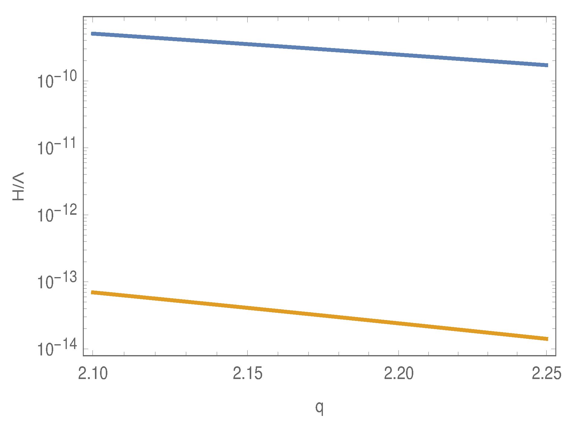
As we have mentioned earlier, the present magnetogenesis scenario predicts sufficient magnetic strength at the current universe when the parameter q lies within . With this information, we give the plots of with respect to q in the range (see Figure 1). The blue curve and yellow curve represent the respective at the beginning of inflation (when ) and at the end of inflation (when , with being the inflationary e-folding number), respectively. In the Figure 1, we take . Figure 1 clearly demonstrates that the ratio during the inflation remains less than unity for the aforementioned range of q, which also leads to the correct magnetic field over the large scale modes at the present epoch of the universe. The following points can be further argued from Figure 1: (a) at the end of inflation obtains a lower value compared to that at the beginning of inflation, and (b) the quantity seems to decrease as the value of q increases. The fact that remains less than unity, i.e., the relevant energy scale of the present model lies well below the cut-off scale, suggests the validity of the proposed theory as an effective field theory. Therefore, the regime of the parameter q, which makes the model viable in regard to the CMB observations of the current magnetic strength and also makes the relevant energy scale of the model below the cut-off scale, is given by .
4. Constraint from Perturbative Requirement
In this section, we derive a bound on the parameter space of the conformal breaking coupling function such that the theory can be treated perturbatively, and the perturbative QFT makes sense. If we expand the metric as , where is the background FRW metric and are the metric perturbations, then the conformal breaking action of Equation (10) introduces non-minimal interaction terms between the graviton and photon. Such interaction Lagrangian is obtained in Equation (28) as
where and are obtained in Equations (25) and (26), respectively. The above interaction terms contribute to the Feynman–Dyson series of the two-point correlator of the EM field, and from the perturbative requirement, we demand that the first terms in the Feynman–Dyson series be small. In particular, the constraint on the coupling function from the perturbative requirement can be derived by either of the following two conditions:
- 1.
- The ratio of the actions for the conformal breaking term to the canonical electromagnetic term should be less than unity [9], i.e.,
- 2.
- The loop contribution in the EM field propagator should be less than that of the tree propagator [65]. In particular,where represents the tree propagator of the EM field, and indicates the loop correction in the EM two-point correlator.
Here we would like to mention that these two conditions are equivalent, as the loop contribution in the EM propagator arises due to the presence of the action .
To examine the first condition in the present context, we start with the following expression of the canonical EM Lagrangian:
where and are the electric and the magnetic energy density, respectively. Consequently, the canonical EM action takes the following form:
with denoting the average over a spatial volume V and being considered to be equivalent to the vacuum expectation value over the Bunch–Davies state (defined in Equation (20) or in Equation (21)). In particular,
For the purpose of determining the , we express in the language of differential forms as
Therefore, the conformal breaking action turns out to be
To arrive at the second equality of the above expression, we use the integration by parts. Considering the comoving observer (having four velocity or ) for measuring the electric and magnetic fields, we find (with being the helicity density) [9]. Accordingly, the becomes
where is given by
Plugging the above expressions back into the left hand side of Equation (37), we arrive at the following equation:
Now, for the condition to be satisfied, it is sufficient to require
Let us denote the ratio in the left hand side of Equation (47) by . Equation (12) immediately leads to as
where is given in Equation (17), due to which can be equivalently expressed as
Moreover, from Equation (20) and Equations (21) and (22), we have the following expressions:
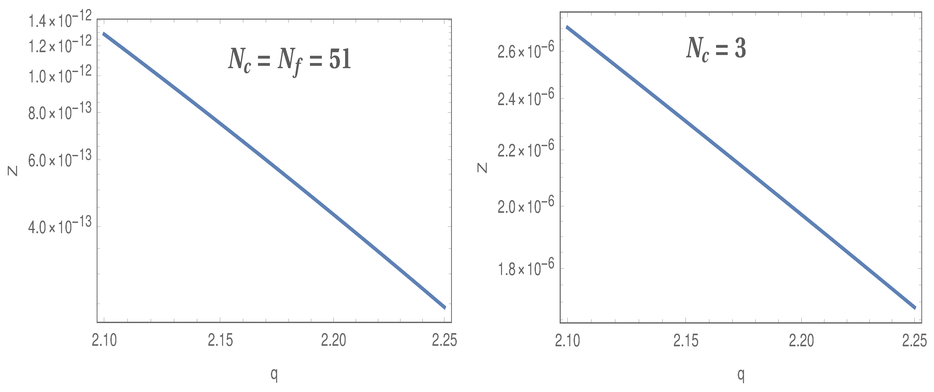
respectively, where () are shown in the Appendix A. The integration limit in Equation (50) is taken from to , i.e., from the mode that crosses the horizon at the beginning of inflation to the mode which crosses the horizon at the instance . Now, we identify the beginning of inflation when the horizon is of the same size as the CMB scale mode, i.e., we may write . Furthermore, we have , with being any time during the inflation, and thus . The quantity is the e-folding number up to measured from the beginning of inflation, i.e., with and . Having obtained the necessary ingredients, we now examine whether the condition is satisfied during inflation. However, due to the dependence of (), the integrations in Equation (50) may not be obtained in analytic form(s), and thus, we numerically approach to integrate , and (at ) present in Equation (50). For this purpose, we consider , and , respectively, and perform the numerical integrations of Equation (50). Consequently, we depict the plot of with respect to the parameter q in the range (see Figure 2). Recall this range of q results to the correct magnetic strength at the present epoch of the universe, and thus, we are using such range of q to examine the perturbative condition in order to keep the generation of the EM field intact. We consider different values of in Figure 2; in particular, we consider and in the left and right plot of Figure 2, respectively. Here, we would like to mention that the mode crosses the horizon near the end of inflation, i.e., , while the mode crosses the horizon near , i.e., near the beginning of inflation.
Figure 2 clearly demonstrates that the perturbative condition is satisfied for , which also leads to the viability of the model with regard to the CMB observations of the current magnetic strength. Therefore, the predictions of perturbative QFT in the model are found to be consistent with the observational bound of the model parameter required to obtain sufficient magnetic strength at the current stage of the universe.
5. Curvature Perturbation Sourced by Electromagnetic Field during Inflation
The produced electromagnetic field during inflation may induce the curvature perturbation [66,67,68,69], and the power spectrum of the induced curvature perturbations should satisfy the recent Planck constraints. Thereby, in the present magnetogenesis scenario where the electromagnetic field couples with the background curvature terms via the dual field tensor, it is important to examine the viability of the sourced curvature perturbations in respect to the Planck constraints.
The induced curvature perturbation (represented by ) from the electromagnetic field is expressed as [66]
where is the background inflaton energy density, and denotes the EM field energy density. Here, it may be mentioned that the contribution from the electromagnetic anisotropic stress is suppressed compared to the contribution written in the r.h.s of Equation (51) (see [69]), and thus, the electromagnetic anisotropic stress in the curvature perturbation is not taken into account in Equation (51). The lower limit of the integral, i.e., , represents the time at which the EM production effectively starts.
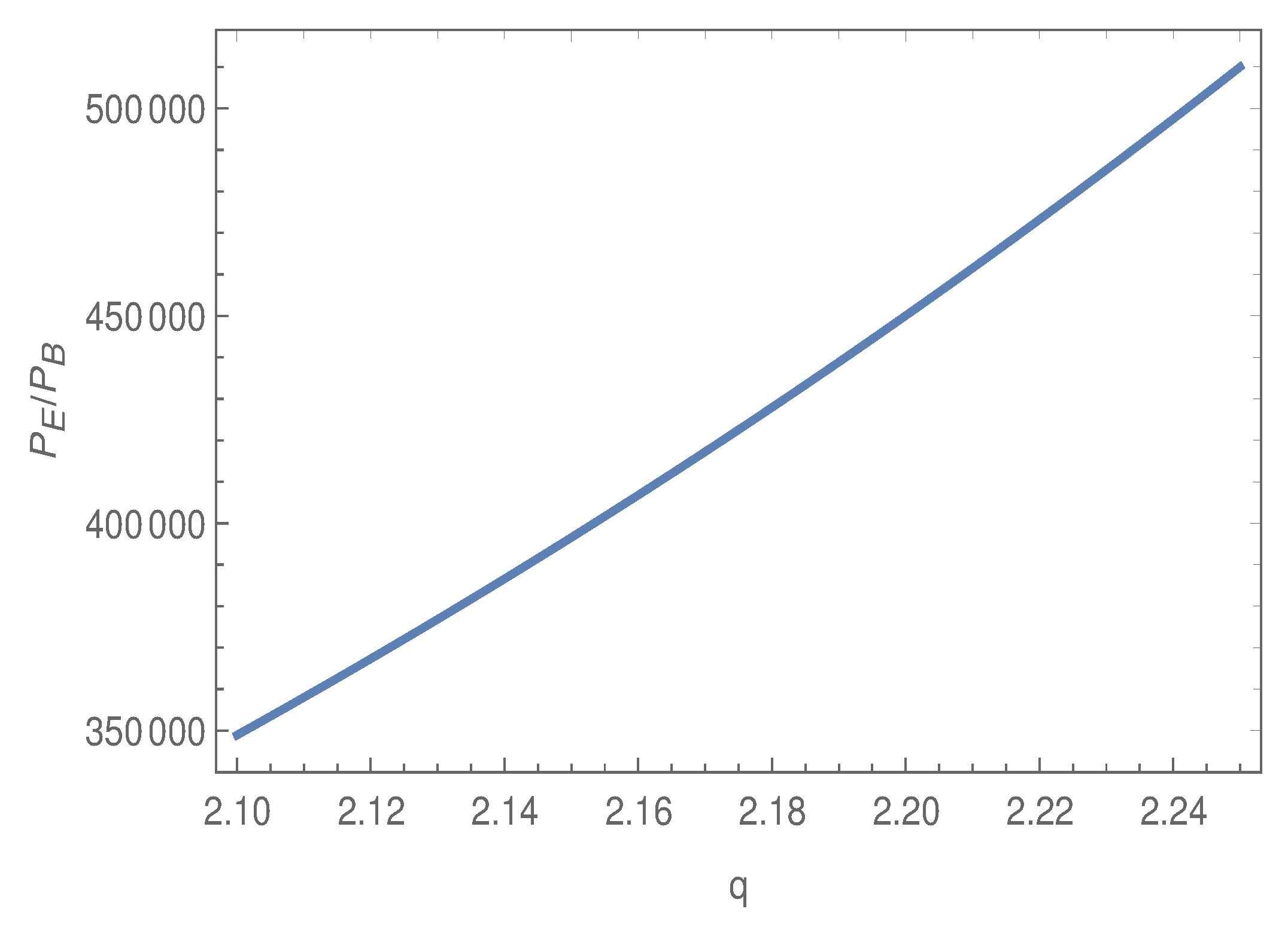
The EM energy density can be expressed by , where and are the energy density for electric and magnetic fields, respectively. However, from Equations (20) and (21), the ratio of the electric to magnetic power spectrum during inflation comes as . In particular, we give the plot of with respect to q in the range in which we are interested (see Figure 3).
The figure clearly depicts that the electric field during inflation is ∼ times stronger than that of the magnetic field strength. This in turn indicates that the main contribution of the EM energy density comes from the electric field, and thus, we may write . Consequently, the EM field energy density in Fourier space is given by
where the electric field is defined as with respect to the comoving observer. Thereby, Equation (19) immediately leads to the electric field as
With the above expression of , we evaluate the two-point correlator of in the present context as [66]:
where and have the following forms:
and
respectively. Here, in Equation (54) represents the mode that crosses the horizon at the end of inflation. Moreover, to derive , we use . Such expression of holds true as the EM field provides a negligible backreaction on the background spacetime in the present magnetogenesis scenario. We may perform the integral of Equation (54) to obtain
where we use the integral . For the momentum variable in the above integral, the corresponding lower limit of the integral is taken as
i.e., when the mode crosses the horizon. This is due to the reason that the EM fluctuations of momentum start to effectively produce from the horizon crossing of . In particular, the energy density stored in a certain mode of the gauge field is maximal (compared to the background energy density) at the horizon crossing of the corresponding mode and then redshifts almost like radiation. Therefore, a certain EM mode is mainly produced near the horizon crossing of that mode in the present magnetogenesis scenario. The consideration of indeed takes care of the horizon crossing region of the mode variable . With and , we evaluate the integral of Equation (57) and obtain
We will eventually evaluate the two point correlator at the CMB scale, and thus, . The above expression of the two-point correlator yields the power spectrum of the curvature perturbation (at ) induced by the EM field as
where the functional forms of or are shown in Equation (56).
Having obtained the theoretical expression of the induced power spectrum at hand, we now confront the model with the Planck results, which put constraint on curvature perturbation as
We consider that the dominant component of the power spectrum of the curvature perturbation is generated by the background slow-roll inflaton field. As a consequence, the theoretical prediction of does not exceed the aforementioned Planck constraint; in particular,
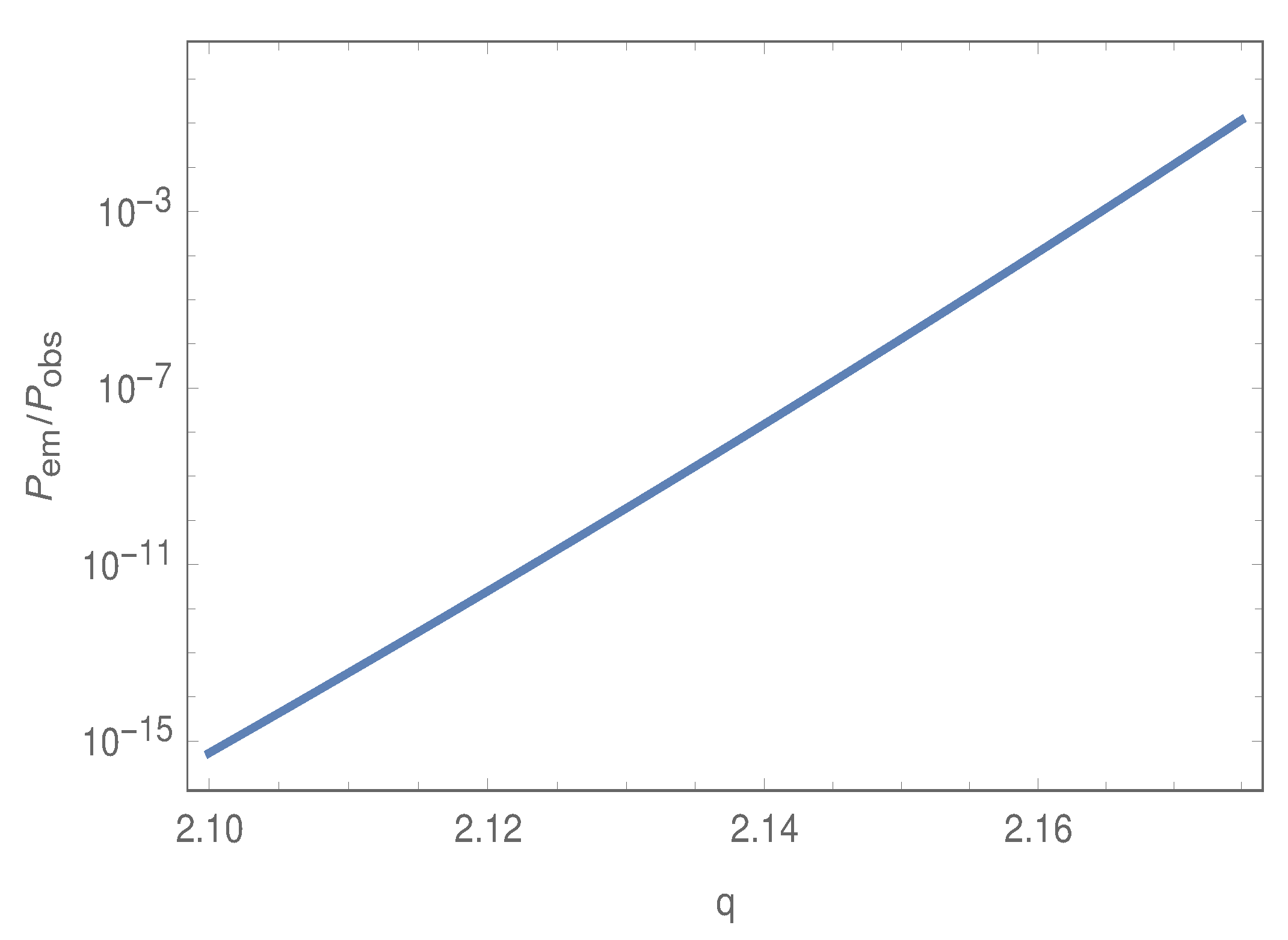
In order to investigate in the present context, we need to evaluate the integral of Equation (60). However, due to the aforementioned form of , this integral may not be obtained in a closed form, so we perform the integration by numerical analysis. This is depicted in Figure 4 where we take the following set of parameters: , , , and . In particular, we plot the ratio of with respect to the parameter q in Figure 4.
Figure 4 clearly demonstrates that in order to satisfy , the parameter q should lie within . Moreover, we recall that the magnetogenesis model under consideration predicts the correct magnetic strength at the present universe for . Therefore, it turns out that the whole range of q which gives the correct magnetic strength does not obey the condition of the induced curvature perturbation, i.e., . In particular, the range of q which leads to a sufficient magnetic strength at the present universe and also ensures is given by .
Before concluding, we would like to mention that some recent studies have argued that non-linear enhancement of the magnetic fields at the end of inflation, inverse cascade of helical photons after inflation, and/or a simultaneous coupling to the photon kinetic term could help increase the strength of the magnetic field [81,82]. Such considerations in the present curvature-coupled helical magnetogenesis scenario will be examined in future work.
6. Conclusions
The recently proposed curvature coupling helical magnetogenesis scenario [7], where the EM field couples with the background gravity, has the following strong features: (1) the model predicts a sufficient magnetic strength at the current epoch of the universe for a suitable range of the model parameter (q) given by for the instantaneous reheating scenario and for the Kamionkowski reheating scenario, respectively; (2) the EM field is found to have a negligible backreaction over the background spacetime and does not jeopardize the background inflation; (3) the model is free from the strong coupling problem; and (4) due to the helical nature of the magnetic field, it turns out that the magnetic strength of ∼ over the galactic scale results in the correct baryon asymmetry of the universe consistent with the observational data.
However, in the realm of inflationary magnetogenesis, the above requirements are not enough to make an argument about the viability of the model. In particular, one needs to examine some more important requirements to ensure the viability of a magnetogenesis model, such as (1) whether the model is consistent with the predictions of perturbative QFT, as the calculations that we use to determine the magnetic field’s evolution and its power spectrum are based on the perturbative QFT; (2) the curvature perturbation sourced by the EM field during inflation should not exceed the curvature perturbation contributed from the background inflaton field, in order to be consistent with the recent Planck data; and (3) the relevant energy scale of the magnetogenesis model needs to lie below the cut-off scale of the model. We have checked all these requirements in the present context of the curvature coupling helical magnetogenesis scenario. For the perturbative requirement, we have examined whether the condition is satisfied, where and are the canonical and the conformal breaking action of the EM field, respectively. The condition actually indicates that the loop contribution of the EM two-point correlator is less than the tree propagator of the EM field, which is the essence of the perturbative quantum field theory. For the second requirement, we have calculated the power spectrum of curvature perturbation sourced by the EM field at super-Hubble scales (). By considering that the primordial curvature perturbation is mainly contributed from the slow-roll inflaton field, we have determined the necessary condition corresponding to the requirement given by , where corresponds to the Planck observation of the curvature perturbation power spectrum. This puts a constraint on the parameter q as . Therefore, it turns out that the whole range of q which gives the correct magnetic strength does not obey the condition of the induced curvature perturbation, i.e., . In particular, the range of q which leads to a sufficient magnetic strength at the present universe and also ensures is given by .
Interestingly, all three aforementioned requirements are found to be simultaneously satisfied by that range of the model parameter which leads to the correct magnetic strength over the large scale modes.
Funding
This research received no external funding.
Institutional Review Board Statement
Not applicable.
Informed Consent Statement
Not applicable.
Data Availability Statement
Not applicable.
Acknowledgments
T.P. sincerely acknowledges Sergei D. Odintsov for useful discussions. This research was supported in part by the International Centre for Theoretical Sciences (ICTS) for the online program Physics of the Early Universe: ICTS/peu2022/1.
Conflicts of Interest
The authors declare no conflict of interest.
Appendix A. Forms of Ci (i = 1, 2, 3, 4)
The solutions of can be demonstrated as follows: in the sub-Hubble scale when , the EM mode functions remain in Bunch–Davies vacuum state, and in the super-Hubble scale when , the are given by Equation (18). Here, are the integration constants which can be determined by matching and at the transition time of sub-Hubble and super-Hubble regimes, i.e., when . If is the horizon crossing instance of the mode k, then we have , where is shown in Equation (5). As a result, the are given by the following expressions [7]:
Similarly,
In the above expressions, and , are shown earlier in Equation (17).
References
- Grasso, D.; Rubinstein, H.R. Magnetic fields in the early universe. Phys. Rep. 2001, 348, 163–266. [Google Scholar] [CrossRef] [Green Version]
- Beck, R. Galactic and extragalactic magnetic fields. Space Sci. Rev. 2001, 99, 243–260. [Google Scholar] [CrossRef]
- Widrow, L.M. Origin of galactic and extragalactic magnetic fields. Rev. Mod. Phys. 2002, 74, 775–823. [Google Scholar] [CrossRef] [Green Version]
- Kulsrud, R.M.; Zweibel, E.G. The Origin of Astrophysical Magnetic Fields. Rep. Prog. Phys. 2008, 71, 46091. [Google Scholar] [CrossRef] [Green Version]
- Brandenburg, A.; Subramanian, K. Astrophysical magnetic fields and nonlinear dynamo theory. Phys. Rep. 2005, 417, 1–209. [Google Scholar] [CrossRef] [Green Version]
- Subramanian, K. Magnetic fields in the early universe. Astron. Nachr. 2010, 331, 110–120. [Google Scholar] [CrossRef] [Green Version]
- Bamba, K.; Odintsov, S.D.; Paul, T.; Maity, D. Helical magnetogenesis with reheating phase from higher curvature coupling and baryogenesis. Phys. Dark Univ. 2022, 36, 101025. [Google Scholar] [CrossRef]
- Jain, R.K.; Sloth, M.S. Consistency relation for cosmic magnetic fields. Phys. Rev. D 2012, 86, 123528. [Google Scholar] [CrossRef] [Green Version]
- Durrer, R.; Hollenstein, L.; Jain, R.K. Can slow roll inflation induce relevant helical magnetic fields? J. Cosmol. Astropart. Phys. 2011, 3, 37. [Google Scholar] [CrossRef] [Green Version]
- Kanno, S.; Soda, J.; Watanabe, M.A. Cosmological Magnetic Fields from Inflation and Backreaction. J. Cosmol. Astropart. Phys. 2009, 12, 9. [Google Scholar] [CrossRef]
- Campanelli, L. Helical Magnetic Fields from Inflation. Int. J. Mod. Phys. D 2009, 18, 1395–1411. [Google Scholar] [CrossRef] [Green Version]
- Demozzi, V.; Mukhanov, V.; Rubinstein, H. Magnetic fields from inflation? J. Cosmol. Astropart. Phys. 2009, 8, 25. [Google Scholar] [CrossRef] [Green Version]
- Demozzi, V.; Ringeval, C. Reheating constraints in inflationary magnetogenesis. J. Cosmol. Astropart. Phys. 2012, 5, 9. [Google Scholar] [CrossRef] [Green Version]
- Bamba, K.; Sasaki, M. Large-scale magnetic fields in the inflationary universe. J. Cosmol. Astropart. Phys. 2007, 2, 30. [Google Scholar] [CrossRef]
- Kobayashi, T.; Sloth, M.S. Early Cosmological Evolution of Primordial Electromagnetic Fields. Phys. Rev. D 2019, 100, 23524. [Google Scholar] [CrossRef] [Green Version]
- Bamba, K.; Elizalde, E.; Odintsov, S.D.; Paul, T. Inflationary magnetogenesis with reheating phase from higher curvature coupling. J. Cosmol. Astropart. Phys. 2021, 4, 9. [Google Scholar] [CrossRef]
- Maity, D.; Pal, S.; Paul, T. Effective Theory of Inflationary Magnetogenesis and Constraints on Reheating. J. Cosmol. Astropart. Phys. 2021, 5, 45. [Google Scholar] [CrossRef]
- Haque, M.R.; Maity, D.; Pal, S. Probing the reheating phase through primordial magnetic field and CMB. arXiv 2021, arXiv:2012.10859. [Google Scholar] [CrossRef]
- Ratra, B. Cosmological ‘seed’ magnetic field from inflation. Astrophys. J. Lett. 1992, 391, L1–L4. [Google Scholar] [CrossRef] [Green Version]
- Ade, P.A.R.; Aghanim, N.; Arnaud, M.; Arroja, F.; Ashdown, M.; Aumont, J.; Baccigalupi, C.; Ballardini, M.; Banday, A.J.; Barreiro, R.B.; et al. Planck 2015 results. XIX. Constraints on primordial magnetic fields. Astron. Astrophys. 2016, 594, A19. [Google Scholar] [CrossRef] [Green Version]
- Chowdhury, D.; Sriramkumar, L.; Kamionkowski, M. Enhancing the cross-correlations between magnetic fields and scalar perturbations through parity violation. J. Cosmol. Astropart. Phys. 2018, 10, 31. [Google Scholar] [CrossRef] [Green Version]
- Turner, M.S.; Widrow, L.M. Inflation Produced, Large Scale Magnetic Fields. Phys. Rev. D 1988, 37, 2743. [Google Scholar] [CrossRef] [PubMed]
- Tripathy, S.; Chowdhury, D.; Jain, R.K.; Sriramkumar, L. Challenges in the choice of the nonconformal coupling function in inflationary magnetogenesis. Phys. Rev. D 2022, 105, 63519. [Google Scholar] [CrossRef]
- Ferreira, R.J.Z.; Jain, R.K.; Sloth, M.S. Inflationary magnetogenesis without the strong coupling problem. J. Cosmol. Astropart. Phys. 2013, 10, 4. [Google Scholar] [CrossRef] [Green Version]
- Atmjeet, K.; Seshadri, T.R.; Subramanian, K. Helical cosmological magnetic fields from extra-dimensions. Phys. Rev. D 2015, 91, 103006. [Google Scholar] [CrossRef] [Green Version]
- Kushwaha, A.; Shankaranarayanan, S. Helical magnetic fields from Riemann coupling. Phys. Rev. D 2020, 102, 103528. [Google Scholar] [CrossRef]
- Gasperini, M.; Giovannini, M.; Veneziano, G. Primordial magnetic fields from string cosmology. Phys. Rev. Lett. 1995, 75, 3796–3799. [Google Scholar] [CrossRef] [Green Version]
- Giovannini, M. Large-scale gauge spectra and pseudoscalar couplings. Phys. Rev. D 2021, 104, 123509. [Google Scholar] [CrossRef]
- Giovannini, M. Baryogenesis, magnetogenesis and the strength of anomalous interactions. Eur. Phys. J. C 2021, 81, 503. [Google Scholar] [CrossRef]
- Adshead, P.; Giblin, J.T.; Scully, T.R.; Sfakianakis, E.I. Gauge-preheating and the end of axion inflation. J. Cosmol. Astropart. Phys. 2015, 12, 34. [Google Scholar] [CrossRef] [Green Version]
- Caprini, C.; Sorbo, L. Adding helicity to inflationary magnetogenesis. J. Cosmol. Astropart. Phys. 2014, 10, 56. [Google Scholar] [CrossRef] [Green Version]
- Kobayashi, T. Primordial Magnetic Fields from the Post-Inflationary Universe. J. Cosmol. Astropart. Phys. 2014, 5, 40. [Google Scholar] [CrossRef] [Green Version]
- Atmjeet, K.; Pahwa, I.; Seshadri, T.R.; Subramanian, K. Cosmological Magnetogenesis From Extra-dimensional Gauss Bonnet Gravity. Phys. Rev. D 2014, 89, 63002. [Google Scholar] [CrossRef] [Green Version]
- Fujita, T.; Namba, R.; Tada, Y.; Takeda, N.; Tashiro, H. Consistent generation of magnetic fields in axion inflation models. J. Cosmol. Astropart. Phys. 2015, 5, 54. [Google Scholar] [CrossRef] [Green Version]
- Campanelli, L. Lorentz-violating inflationary magnetogenesis. Eur. Phys. J. C 2015, 75, 278. [Google Scholar] [CrossRef] [Green Version]
- Tasinato, G. A scenario for inflationary magnetogenesis without strong coupling problem. J. Cosmol. Astropart. Phys. 2015, 3, 40. [Google Scholar] [CrossRef] [Green Version]
- Frion, E.; Pinto-Neto, N.; Vitenti, S.D.P.; Bergliaffa, S.E.P. Primordial Magnetogenesis in a Bouncing Universe. Phys. Rev. D 2020, 101, 103503. [Google Scholar] [CrossRef]
- Koley, R.; Samtani, S. Magnetogenesis in Matter—Ekpyrotic Bouncing Cosmology. J. Cosmol. Astropart. Phys. 2017, 4, 30. [Google Scholar] [CrossRef] [Green Version]
- Qian, P.; Cai, Y.F.; Easson, D.A.; Guo, Z.K. Magnetogenesis in bouncing cosmology. Phys. Rev. D 2016, 94, 83524. [Google Scholar] [CrossRef] [Green Version]
- Guth, A.H. Inflationary universe: A possible solution to the horizon and flatness problems. Phys. Rev. D 1981, 23, 347–356. [Google Scholar] [CrossRef] [Green Version]
- Linde, A.D. Particle physics and inflationary cosmology. Contemp. Concepts Phys. 1990, 5, 1. [Google Scholar]
- Langlois, D. Inflation, quantum fluctuations and cosmological perturbations. arXiv 2004, arXiv:hep-th/0405053. [Google Scholar]
- Riotto, A. Inflation and the theory of cosmological perturbations. ICTP Lect. Notes Ser. 2003, 14, 317. [Google Scholar]
- Baumann, D. Inflation. arXiv 2009, arXiv:0907.5424. [Google Scholar]
- Nandi, D. Inflationary magnetogenesis: Solving the strong coupling and its non-Gaussian signatures. J. Cosmol. Astropart. Phys. 2021, 8, 39. [Google Scholar] [CrossRef]
- Dai, L.; Kamionkowski, M.; Wang, J. Reheating constraints to inflationary models. Phys. Rev. Lett. 2014, 113, 41302. [Google Scholar] [CrossRef] [Green Version]
- Cook, J.L.; Dimastrogiovanni, E.; Easson, D.A.; Krauss, L.M. Reheating predictions in single field inflation. J. Cosmol. Astropart. Phys. 2015, 4, 47. [Google Scholar] [CrossRef]
- Albrecht, A.; Steinhardt, P.J.; Turner, M.S.; Wilczek, F. Reheating an Inflationary Universe. Phys. Rev. Lett. 1982, 48, 1437. [Google Scholar] [CrossRef]
- Ellis, J.; Garcia, M.A.G.; Nanopoulos, D.V.; Olive, K.A. Calculations of Inflaton Decays and Reheating: With Applications to No-Scale Inflation Models. J. Cosmol. Astropart. Phys. 2015, 7, 50. [Google Scholar] [CrossRef]
- Ueno, Y.; Yamamoto, K. Constraints on α-attractor inflation and reheating. Phys. Rev. D 2016, 93, 83524. [Google Scholar] [CrossRef] [Green Version]
- Eshaghi, M.; Zarei, M.; Riazi, N.; Kiasatpour, A. CMB and reheating constraints to α-attractor inflationary models. Phys. Rev. D 2016, 93, 123517. [Google Scholar] [CrossRef] [Green Version]
- Maity, D.; Saha, P. (P)reheating after minimal Plateau Inflation and constraints from CMB. J. Cosmol. Astropart. Phys. 2019, 7, 18. [Google Scholar] [CrossRef] [Green Version]
- Haque, M.R.; Maity, D.; Paul, T.; Sriramkumar, L. Decoding the phases of early and late time reheating through imprints on primordial gravitational waves. Phys. Rev. D 2021, 104, 63513. [Google Scholar] [CrossRef]
- Marco, A.D.; Cabella, P.; Vittorio, N. Constraining the general reheating phase in the α-attractor inflationary cosmology. Phys. Rev. D 2017, 95, 103502. [Google Scholar] [CrossRef] [Green Version]
- Drewes, M.; Kang, J.U.; Mun, U.R. CMB constraints on the inflaton couplings and reheating temperature in α-attractor inflation. J. High Energy Phys. 2017, 11, 72. [Google Scholar] [CrossRef] [Green Version]
- Nojiri, S.; Odintsov, S.D.; Sasaki, M. Gauss-Bonnet dark energy. Phys. Rev. D 2005, 71, 123509. [Google Scholar] [CrossRef] [Green Version]
- Li, B.; Barrow, J.D.; Mota, D.F. The Cosmology of Modified Gauss-Bonnet Gravity. Phys. Rev. D 2007, 76, 44027. [Google Scholar] [CrossRef] [Green Version]
- Carter, B.M.; Neupane, I.P. Towards inflation and dark energy cosmologies from modified Gauss-Bonnet theory. J. Cosmol. Astropart. Phys. 2006, 6, 4. [Google Scholar] [CrossRef] [Green Version]
- Nojiri, S.; Odintsov, S.; Oikonomou, V.; Chatzarakis, N.; Paul, T. Viable inflationary models in a ghost-free Gauss–Bonnet theory of gravity. Eur. Phys. J. C 2019, 79, 565. [Google Scholar] [CrossRef] [Green Version]
- Cognola, G.; Elizalde, E.; Nojiri, S.; Odintsov, S.D.; Zerbini, S. Dark energy in modified Gauss-Bonnet gravity: Late-time acceleration and the hierarchy problem. Phys. Rev. D 2006, 73, 84007. [Google Scholar] [CrossRef] [Green Version]
- Chakraborty, S.; Paul, T.; SenGupta, S. Inflation driven by Einstein-Gauss-Bonnet gravity. Phys. Rev. D 2018, 98, 83539. [Google Scholar] [CrossRef] [Green Version]
- Elizalde, E.; Odintsov, S.D.; Oikonomou, V.K.; Paul, T. Extended matter bounce scenario in ghost free gravity compatible with GW170817. Nucl. Phys. B 2020, 954, 114984. [Google Scholar] [CrossRef]
- Nojiri, S.; Odintsov, S.D.; Paul, T. Towards a smooth unification from an ekpyrotic bounce to the dark energy era. Phys. Dark Univ. 2022, 35, 100984. [Google Scholar] [CrossRef]
- Odintsov, S.D.; Paul, T. Bounce universe with finite-time singularity. arXiv 2022, arXiv:2205.09447. [Google Scholar]
- Ferreira, R.Z.; Ganc, J.; Norena, J.; Sloth, M.S. On the validity of the perturbative description of axions during inflation. J. Cosmol. Astropart. Phys. 2016, 4, 39, Erratum in JCAP 2016, 10, E01. [Google Scholar] [CrossRef]
- Fujita, T.; Yokoyama, S. Higher order statistics of curvature perturbations in IFF model and its Planck constraints. J. Cosmol. Astropart. Phys. 2013, 9, 9. [Google Scholar] [CrossRef] [Green Version]
- Barnaby, N.; Namba, R.; Peloso, M. Observable non-gaussianity from gauge field production in slow roll inflation, and a challenging connection with magnetogenesis. Phys. Rev. D 2012, 85, 123523. [Google Scholar] [CrossRef] [Green Version]
- Bamba, K. Generation of large-scale magnetic fields, non-Gaussianity, and primordial gravitational waves in inflationary cosmology. Phys. Rev. D 2015, 91, 43509. [Google Scholar] [CrossRef] [Green Version]
- Suyama, T.; Yokoyama, J. Metric perturbation from inflationary magnetic field and generic bound on inflation models. Phys. Rev. D 2012, 86, 23512. [Google Scholar] [CrossRef] [Green Version]
- Shankaranarayanan, S.; Sriramkumar, L. Trans-Planckian corrections to the primordial spectrum in the infrared and the ultraviolet. Phys. Rev. D 2004, 70, 123520. [Google Scholar] [CrossRef] [Green Version]
- del Campo, S.; Gonzalez, C.; Herrera, R. Power law inflation with a non-minimally coupled scalar field in light of Planck 2015 data: The exact versus slow roll results. Astrophys. Space Sci. 2015, 358, 31. [Google Scholar] [CrossRef] [Green Version]
- Sharma, A.K.; Verma, M.M. Power-law Inflation in the f(R) Gravity. Astrophys. J. 2022, 926, 29. [Google Scholar] [CrossRef]
- Pham, T.M.; Nguyen, D.H.; Do, T.Q. k-Gauss-Bonnet inflation. arXiv 2021, arXiv:2107.05926. [Google Scholar]
- Anber, M.M.; Sorbo, L. N-flationary magnetic fields. J. Cosmol. Astropart. Phys. 2006, 10, 18. [Google Scholar] [CrossRef]
- Barnaby, N.; Namba, R.; Peloso, M. Phenomenology of a Pseudo-Scalar Inflaton: Naturally Large Nongaussianity. J. Cosmol. Astropart. Phys. 2011, 4, 9. [Google Scholar] [CrossRef] [Green Version]
- Peloso, M.; Sorbo, L.; Unal, C. Rolling axions during inflation: Perturbativity and signatures. J. Cosmol. Astropart. Phys. 2016, 9, 1. [Google Scholar] [CrossRef] [Green Version]
- Guendelman, E.I.; Owen, D.A. Axion driven baryogenesis. Phys. Lett. B 1992, 276, 108–114. [Google Scholar] [CrossRef]
- Burgess, C.P.; Lee, H.M.; Trott, M. Power-counting and the Validity of the Classical Approximation During Inflation. J. High Energy Phys. 2009, 9, 103. [Google Scholar] [CrossRef] [Green Version]
- Hertzberg, M.P. On Inflation with Non-minimal Coupling. J. High Energy Phys. 2010, 11, 23. [Google Scholar] [CrossRef] [Green Version]
- Bezrukov, F.; Magnin, A.; Shaposhnikov, M.; Sibiryakov, S. Higgs inflation: Consistency and generalisations. J. High Energy Phys. 2011, 1, 16. [Google Scholar] [CrossRef] [Green Version]
- Adshead, P.; Giblin, J.T.; Scully, T.R.; Sfakianakis, E.I. Magnetogenesis from axion inflation. J. Cosmol. Astropart. Phys. 2016, 10, 39. [Google Scholar] [CrossRef] [Green Version]
- Fujita, T.; Durrer, R. Scale-invariant Helical Magnetic Fields from Inflation. J. Cosmol. Astropart. Phys. 2019, 9, 8. [Google Scholar] [CrossRef] [Green Version]
Figure 1.
versus q in the range , with , , , and . The blue curve represents the ratio of at the beginning of inflation when , and the yellow curve specifies at the end of inflation when .
Figure 1.
versus q in the range , with , , , and . The blue curve represents the ratio of at the beginning of inflation when , and the yellow curve specifies at the end of inflation when .

Figure 2.
vs q for , , and . Moreover, we take . In the (left plot), , which crosses the horizon near the end of inflation, i.e., , while for the (right plot), , which crosses the horizon near , i.e., near the beginning of inflation.
Figure 2.
vs q for , , and . Moreover, we take . In the (left plot), , which crosses the horizon near the end of inflation, i.e., , while for the (right plot), , which crosses the horizon near , i.e., near the beginning of inflation.

Figure 3.
vs. q in the range . Here, we consider , , and . Moreover, we take .

Figure 4.
vs q. Here, we consider , , and . Moreover, we take .

Publisher’s Note: MDPI stays neutral with regard to jurisdictional claims in published maps and institutional affiliations. |
© 2022 by the author. Licensee MDPI, Basel, Switzerland. This article is an open access article distributed under the terms and conditions of the Creative Commons Attribution (CC BY) license (https://creativecommons.org/licenses/by/4.0/).
Share and Cite
MDPI and ACS Style
Paul, T. Viable Requirements of Curvature Coupling Helical Magnetogenesis Scenario. Symmetry 2022, 14, 1086. https://doi.org/10.3390/sym14061086
AMA Style
Paul T. Viable Requirements of Curvature Coupling Helical Magnetogenesis Scenario. Symmetry. 2022; 14(6):1086. https://doi.org/10.3390/sym14061086
Chicago/Turabian StylePaul, Tanmoy. 2022. "Viable Requirements of Curvature Coupling Helical Magnetogenesis Scenario" Symmetry 14, no. 6: 1086. https://doi.org/10.3390/sym14061086
Note that from the first issue of 2016, this journal uses article numbers instead of page numbers. See further details here.