Research on Prediction Method of Gear Pump Remaining Useful Life Based on DCAE and Bi-LSTM

Abstract

As a hydraulic pump is the power source of a hydraulic system, predicting its remaining useful life (RUL) can effectively improve the operating efficiency of the hydraulic system and reduce the incidence of failure. This paper presents a scheme for predicting the RUL of a hydraulic pump (gear pump) through a combination of a deep convolutional autoencoder (DCAE) and a bidirectional long short-term memory (Bi-LSTM) network. The vibration data were characterized by the DCAE, and a health indicator (HI) was constructed and modeled to determine the degradation state of the gear pump. The DCAE is a typical symmetric neural network, which can effectively extract characteristics from the data by using the symmetry of the encoding network and decoding network. After processing the original vibration data segment, health indicators were entered as a label into the RUL prediction model based on the Bi-LSTM network, and model training was carried out to achieve the RUL prediction of the gear pump. To verify the validity of the methodology, a gear pump accelerated life experiment was carried out, and whole life cycle data were obtained for method validation. The results show that the constructed HI can effectively characterize the degenerative state of the gear pump, and the proposed RUL prediction method can effectively predict the degeneration trend of the gear pump.

1. Introduction

With the dramatic growth of the machinery industry, humans have put forward higher requirements for the reliability of machinery and equipment [1]. Hydraulic equipment is extensively used in construction machinery, and the remaining useful life (RUL) prediction method of hydraulic components can effectively improve the reliability of the entire hydraulic equipment and its system [2]. As a typical hydraulic pump, the gear pump has the strengths of having a small size, light weight, reliable operation and wide speed range. As the power source of a hydraulic system, the gear pump is widely used in various hydraulic systems. However, a gear pump usually works in the case of high-speed overload, its operating environment is generally harsh, and its working intensity is high [3]. These factors will undoubtedly have a great impact on the life of the gear pump, and once a failure happens, it will impact the normal function of the entire hydraulic installation. The RUL prediction of a gear pump can effectively improve production efficiency and reduce equipment life cycle costs, thereby reducing the incidence of failure [4].

Deep learning has become a major tool for solving big data problems. Many scholars have applied deep models to the fields of computer vision, natural language processing and disease analysis with good results [5,6,7]. With the galloping growth of industrial Internet of Things technology, the amount of mechanical equipment status-monitoring data is increasing, and on the basis of massive data support, the predictive maintenance of equipment has become the current research hotspot in equipment management [8,9]. As one of the core parts of many types of hydraulic equipment, the working state of the hydraulic pump is directly related to whether the entire equipment can operate safely and stably. Intelligent algorithms based on deep learning have become an important approach in the areas of prognostic health management (PHM), driven by massive industrial state-monitoring data and growing computing power [10,11,12,13,14]. Generally speaking, for the hydraulic pump (gear pump), once a failure occurs, the failure is often reflected in certain feature signals. Deep-learning-based lifetime prediction models can effectively analyze and process these feature signals.

At present, based on signal processing technology, many researchers have studied the condition monitoring and RUL prediction of hydraulic equipment. R. Guo et al. used the Bayesian regularized radial basis function neural network to predict the RUL of a gear pump [15]. X. Liang et al. used multivariate signals as data samples to realize fault diagnosis of a hydraulic pump through a sparse autoencoder [16]. Z. Li et al. used data dimension reduction and just-in-time learning techniques to analyze the pressure signal to predict the RUL of a hydraulic pump [17]. S. Tang et al. presented an intelligent fault diagnosis method based on the combination of a convolutional neural network (CNN) and the continuous wavelet transform (CWT), which can diagnose hydraulic pump faults through vibration signals [18]. H. Chen et al. used parallel factor-improved particle swarm algorithm (IPSO)-probabilistic neural network (PNN)-driven multi-sensor data to identify the nonstationary multi-fault mode of a centrifugal pump [19]. H. Tang et al. proposed a fault diagnosis approach for the loose slipper failure of a piston pump under variable load. The vibration signals of the axial piston pump are collected, and the root mean square value of each segment of the signal is calculated to obtain the trend line of the root mean square gradient. Finally, the trend line of the loose slipper failure detection is based on the gradient [20]. Y. Lan et al. extracted the features of the vibration signals of a hydraulic pump and classified the features through the improved extreme learning machine (ELM) to achieve fault diagnosis [21]. H. Babikir et al. predicted axial piston pump noise based on an improved artificial neural network model for different valve materials [22]. W. Jiang et al. extracted the features of the sound signal of an axial piston pump based on mel-frequency cepstrum coefficients (MFCCs). Extreme learning machine was used as a classifier to diagnose faults from sound features [23]. Y. Zhu et al. used CNN to classify the two-dimensional time-frequency diagram of vibration data to achieve the fault diagnosis of a hydraulic pump [24]. Most hydraulic pumps belong to rotating machinery equipment. As the machinery industry is also moving towards the era of big data, deep learning is being widely used in fault diagnosis and life prediction of rotating machinery devices [25]. Many researchers have improved common deep learning models, such as CNN, long short-term memory (LSTM), deep belief network (DBN) and generative adversarial networks (GANs), and have demonstrated good effectiveness in pattern recognition of rotating machinery [26,27,28,29,30,31]. The research results show that deep learning has broad application prospects in the field of mechanical equipment PHM.

However, there are still many problems that need to be solved in RUL prediction for hydraulic pumps. In the data acquisition stage, the traditional life test has problems such as a long test cycle, difficulty in data acquisition and difficulty in simulating extreme working conditions of the equipment. Currently, there are few hydraulic pump life datasets available, making it difficult to perform effective model training. In the data analysis stage, how to obtain valuable data from it against the background of large and complex monitoring data and how to effectively moderate the degradation state of the hydraulic pump are urgent problems to solve. During the RUL prediction model training phase, the training accuracy of the remaining life prediction model is also closely related to two factors: one is the correct choice of the model, and the other is the quality of the data required to train the model. The correct selection of the algorithm and the high and low quality of the training data also directly affect the predictive accuracy of the model.

This paper uses a gear pump as the research object. The RUL scheme consists of two segments, as illustrated in Figure 1. The first part represents the steps of modeling the degradation state of the gear pump. By combining a deep convolutional autoencoder (DCAE) with a self-organizing map network, effective feature abstraction of the original vibration signal is used to construct the gear pump health indicator (HI). The second part represents the gear pump life prediction model. The HI values are added as labels to the original data to form the training set, and then the Bi-LSTM model is trained. The output of the model is the prediction of the RUL of the gear pump.

The paper is arranged as given below. Section 2 introduces the degradation state of the gear pump and the required deep learning method. Section 3 proposes an accelerated life experiment scheme for the gear pump. Section 4 introduces the method of degradation state modeling of the gear pump based on a DCAE and a self-organizing map (SOM). Section 5 proposes a RUL prediction model of the gear pump based on Bi-LSTM. Section 6 is the conclusion.

2. Theoretical Background

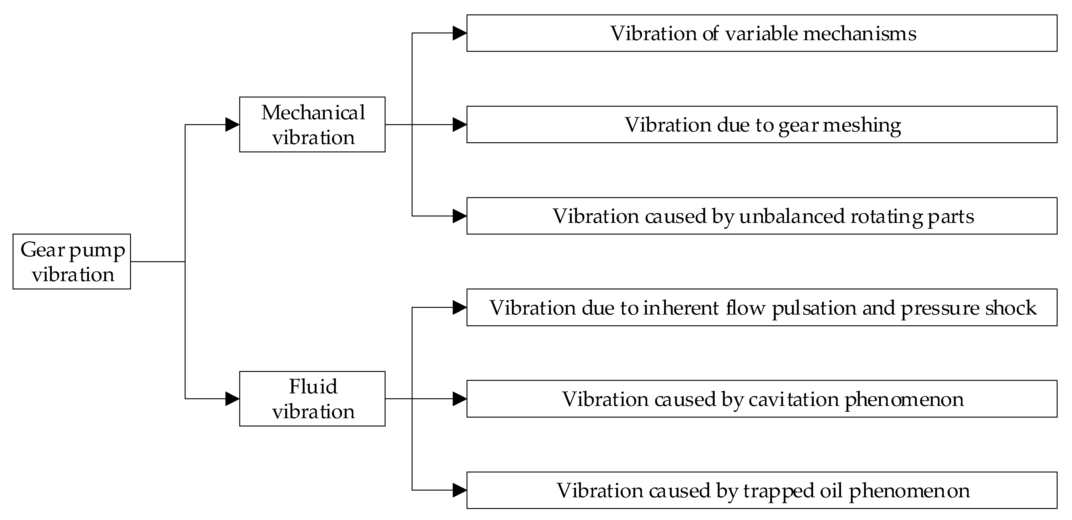
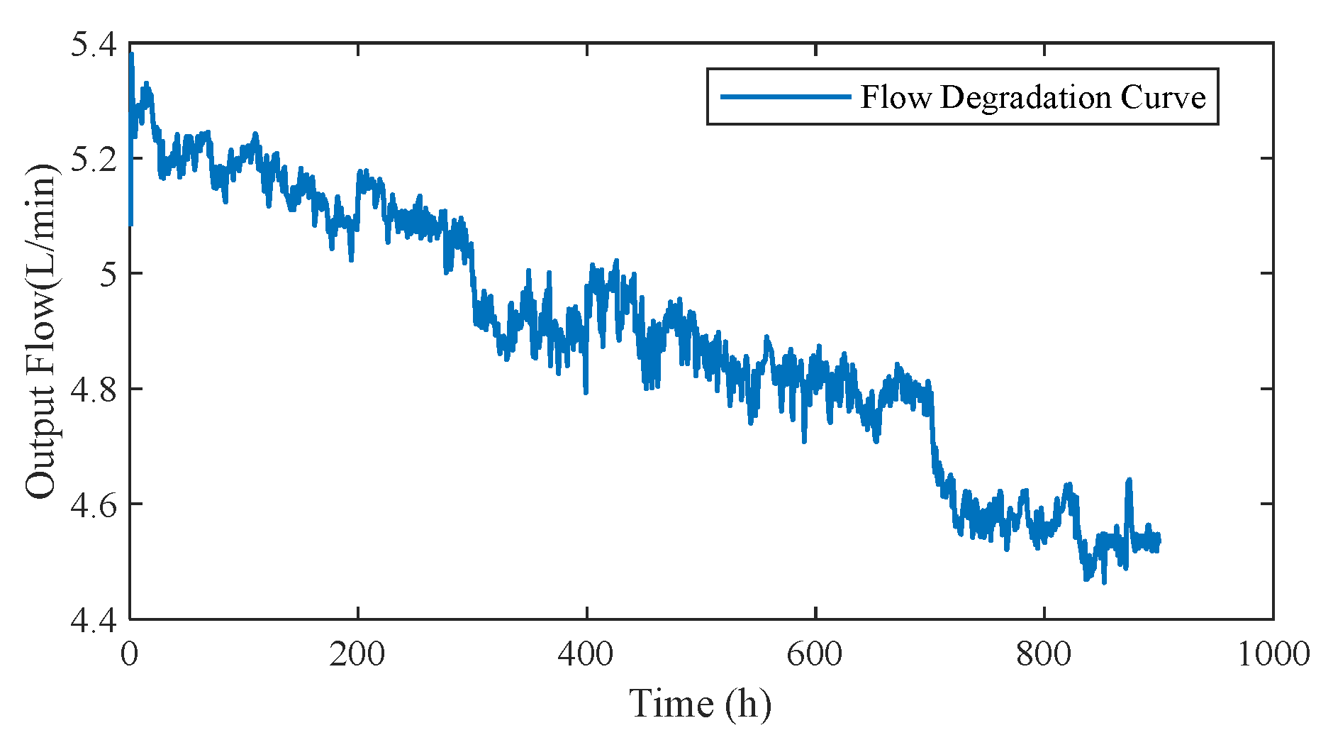
2.1. Degradation Analysis of Gear Pump

The main failure mode of a gear pump is fatigue and wear, where fatigue failure occurs in the parts that bear repeated alternate loads, and wear failure occurs in the parts that bear repeated friction. The common wear parts of a gear pump are the gear end and floating side plate, tooth and shell inner cavity, gear tooth surface, etc. With the increase in use time, key performance characteristics (such as oil flow back) gradually degrade. When the performance characteristics degrade beyond the predetermined failure threshold, the hydraulic pump fails. Degradation data of key performance characteristics can be used to assess the reliability of hydraulic pumps [32,33]. Gear pumps belong to typical rotating machinery; the structure and fluid will cause the vibration of the gear pump, reflected in mechanical vibration and fluid vibration, as shown in Figure 2. When the device is in a failure state, the quality, stiffness and damping of the system will change, and these changes will be reflected in the vibration signal. This paper analyzes the degradation state and predicts the RUL according to the vibration data of the gear pump.

2.2. Autoencoder (AE)

An autoencoder (AE) is an unsupervised learning model, whose functions are to take the input information as the learning target and carry out representational learning. AE is a neural network that consists of input layers, hidden layers and output layers, and neurons in different layers are connected in a fully connected manner. The output layer and input layer in AE usually have more neurons than the hidden layer; this construction is known as an imperfect AE. Imperfect learning refers to the need for AE to capture the significant characteristics of data to achieve the effect of characteristic parsimony [34]. Autoencoders provide a way to perform unsupervised and semi-supervised learning. Rotating mechanical devices have a long life cycle and usually contain a large amount of unlabeled data information. The feature extraction process for these data falls under the category of unsupervised and semi-supervised learning.

In this paper, the encoding network and decoding network are expressed by $h=g(x)$ and $r=\phi (\mathit{h})$, where $x$ and $r$ are the input and output of the AE. Its optimization goal can be formulated as $\min J(x,r)$. $J$ is the loss function, which is usually the mean square error.

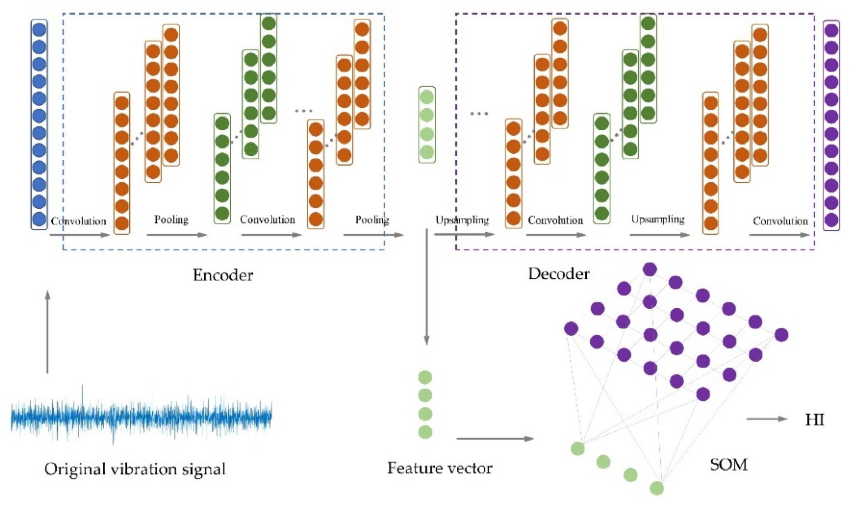
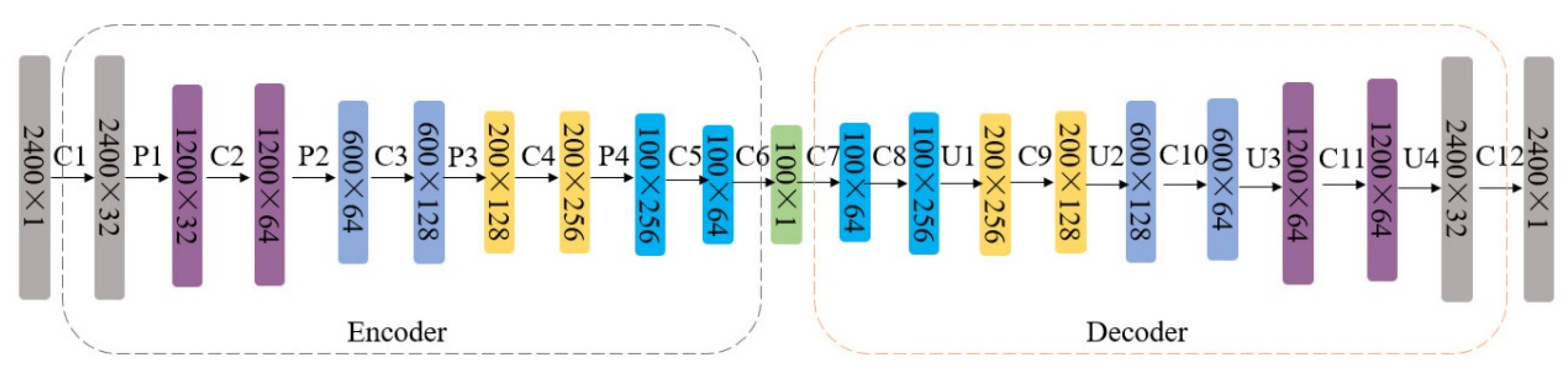
Convolutional Autoencoder (CAE)

The convolutional autoencoder is an extension of the traditional AE, which replaces the ordinary matrix inner product with the convolution operation [35]. The CAE not only enhances the nonlinear mapping ability of the AE but also enhances its ability to extract spatially related information. The DCAE constructed in this paper exploits the symmetry in AE. The encoder and the decoder have the same structure and can effectively extract the features of the vibration signal based on their symmetry characteristics.

2.3. Convolutional Neural Network (CNN)

The two most important parts of a traditional CNN are the convolutional layer and the pooling layer [36,37]. CNN has three core ideas: parameter sharing, equivalence denotation and sparse interaction. These features of CNN are ideal for handling big data. The gear pump has a long life cycle and a large amount of data, and the data type is a non-smooth one-dimensional time series. In this paper, the AE is improved by a one-dimensional convolution kernel to make the AE more suitable for processing one-dimensional time series of vibration data. Convolution is used to reconcile the output characteristic vector of the previous layer and to construct the output characteristic vector using the nonlinear activation function. The network can be expressed as:

$$x_j^l=f\left({\displaystyle \sum _{i\in M_j}{x}_i^{l-1}}\times k_{ij}^l+b_j^l\right)$$

(1)

where $b$ is the bias vector, $x_j^l$ and $x_i^{l-1}$ stand for the output and input of the $l$-th layer, respectively, $k$ is the convolution kernel, and $M_j$ is the input feature vector.

The pooling layer is proposed to alleviate the excessive sensitivity of the convolutional layer to position. Pooling is a form of sampling under nonlinearity, reducing computation by reducing the parameters of the network. Maximum pooling is the division of the input layer into different areas using rectangular boxes that do not overlap, so each rectangular box maximizes the output layer. The maximum pooling is denoted as:

$$P_i^{l+1}(j)=\underset{(j-1)U+1\le n\le jU}{\max }\left\{v_i^l(n)\right\}$$

(2)

where $n\in [(j-1)U+1,jU]$, $U$ is the width of the pooling zones, $P_i^{l+1}(j)$ is the value of neurons in the $(l+1)$-th layer, and $v_i^l(n)$ is the value of the $n$-th neuron in the $i$-th feature vector of the $l$-th layer.

2.4. Self-Organizing Map (SOM) Network

A SOM network is an unsupervised learning network. It automatically changes the network parameters and structure through self-organization and self-adaptation by automatically searching the intrinsic laws and natural properties of the data. By learning the data in the input space, SOM produces a low-dimensional and outlying map. To a certain extent, it can also be regarded as a dimension reduction algorithm. SOM is a typical self-organizing neural network with an input layer and competition layer. The input layer accepts external information and transmits the input pattern to the competition layer; the competition layer is responsible for “analyzing and comparing” the input pattern, looking for rules and classifying them.

2.5. Long Short-Term Memory (LSTM)

An LSTM network is a peculiar kind of recurrent neural network (RNN) proposed by researchers according to performance requirements [38]. By introducing gating units, LSTM can dynamically change the accumulated time scale to better handle time-series data. In LSTM, $x$, $h$ and $y$ are the input layer, hidden layer and output layer of the network. At time $t$, its input is not only $x_t$ but also the output of the previous time step $h_{t-1}$. The specific expression is

$$h_t=f(U\cdot x_t+W\cdot h_{t-1}+b_h)$$

(3)

$$y_t=V\cdot h_t+b_y$$

(4)

where $f$ is the nonlinear activation function; $W$, $U$ and $V$ are weight coefficient matrices, which are shared at different times and do not change with time; and $b_h$ and $b_y$ are the bias vectors of the hidden layer and output layer.

Figure 3 is the basic structure of the LSTM unit. In order to realize the control and flow of storage memory, LSTM introduces three gate units: the forget gate, input gate and output gate. By introducing gate units, it is easier for LSTM networks to learn long-term dependencies than ordinary RNN. The forget gate is used to decide which information to keep in the status unit, and the specific mathematical expression is

$$f_t=\sigma \left(W_f[h_{t-1},x_t]+b_f\right)$$

(5)

where $\sigma$ is generally a sigmoid function, and $[h_{t-1},x_t]$ is the concatenation of the state of the previous time step and the input at this moment.

The input gate is used to determine the input information, and its expression is

$$i_t=\sigma \left(W_i[h_{t-1},x_t]+b_f\right)$$

(6)

$${\tilde{C}}_t=\tanh \left(W_c[h_{t-1},x_t]+b_c\right)$$

(7)

The results obtained by the forget gate and the input gate are united to update the long-term memory unit $C$, and the definition is as follows:

$$C_t=f_t\odot C_{t-1}+i_t\odot {\tilde{C}}_t$$

(8)

In the formula, $f_t\odot C_{t-1}$ represents the multiplication of each element of the forget gate and the corresponding element of the long-term memory state at the previous moment, which is used to forget part of the information of the long-term memory state. $i_t\odot {\tilde{C}}_t$ is used to select the current input information and then accumulate it into the long-term memory state. The end output of the LSTM unit is controlled via the output gate $o_t$, and its expression is defined as follows:

$$o_t=\sigma \left(W_o[h_{t-1},x_t]+b_o\right)$$

(9)

$$h_t=o_t\odot \tanh (C_t)$$

(10)

The basic idea of the RNN-based method for RUL prediction is to use the input of monitoring data from the project as the input of the RNN and to use the training of the model parameters through time backpropagation to achieve the RUL prediction of the equipment. It should be noted that the internal feedback connection of the RNN portrays the before-and-after dependence of the monitoring data. The LSTM determines whether to preserve the existing information through the structure of the three gates, a feature that makes it more suitable for dealing with the prediction problem of long-term data. The amount of data for the whole life cycle of a gear pump is very large. RUL prediction based on LSTM can effectively reduce problems such as gradient disappearance and gradient explosion faced by RNN models with large datasets.

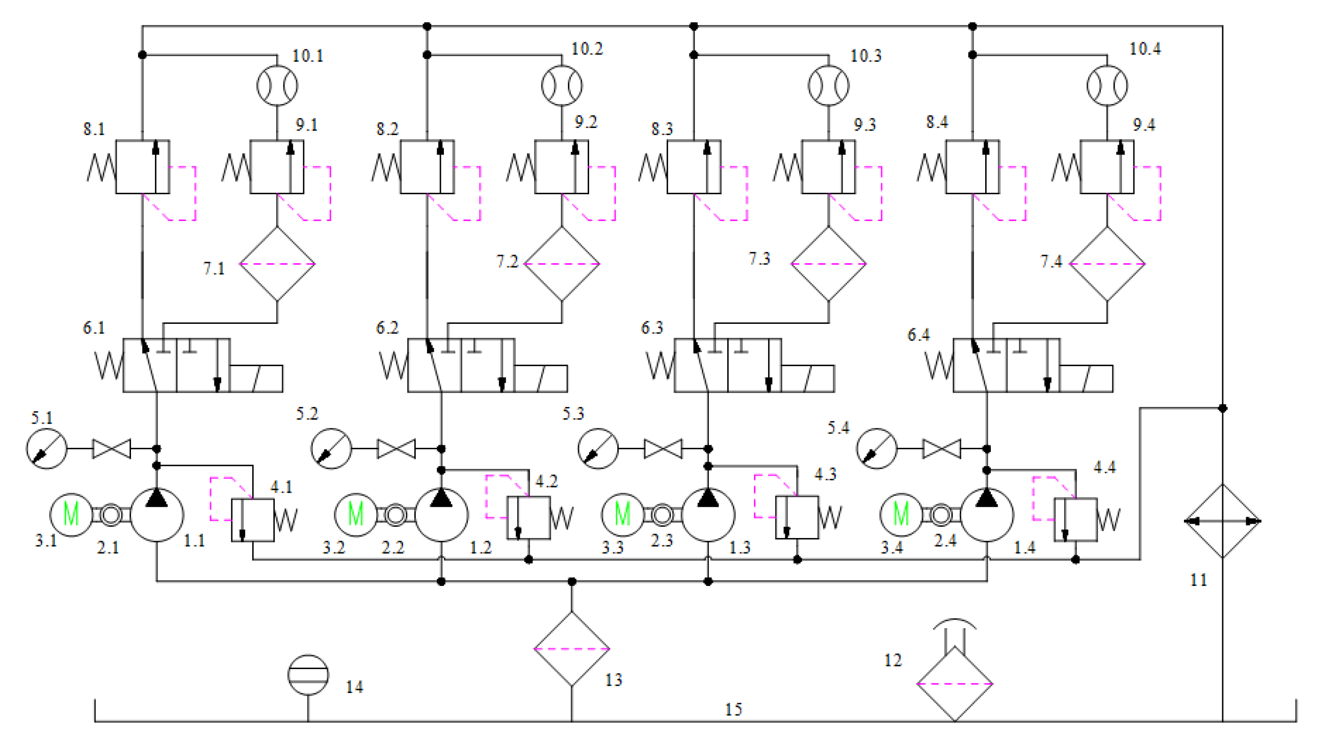
3. Experimental Settings

The experiment was an accelerated life test with four gear pumps operating at higher-than-rated pressures the majority of the time. However, the test pressure needs to be adjusted to the rated operating pressure of the pump when collecting data, so each gear pump has two branches: the high-pressure acceleration branch and the rated operating pressure branch. During the experiment, the rated operating pressure branch is only entered during data acquisition, and the rest of the time, it is under the high-pressure acceleration branch. When the signal acquisition is carried out, the reversing valve operates and enters the rated working pressure branch, and the acquisition starts after the flow is stabilized. In order to reduce the impact of hydraulic oil temperature changes during the experiment, a PLC-controlled fan is used. When the set hydraulic oil temperature is greater than 49 °C, the fan starts to reduce the oil temperature, and when the oil temperature is lower than 49 °C, the fan stops rotating; the purpose is to ensure that the oil temperature is controlled at around 50 °C. During the experiment, the safety pressure of all four safety valves was set to 30 MPa in order to ensure the safety of the experiment.

This life acceleration test bench was used to conduct experiments on 4 gear pumps of the same type at the same time. The sensors installed in the test include torque sensors, flow meters and acceleration sensors to monitor and collect changes in torque, rotational speed, output flow and vibration throughout the life test. The test bench can make the gear pump work under non-rated conditions so that the gear pump accelerates its wear and degradation. The change in pumps’ pressure is mainly controlled by the low-pressure relief valve. The schematic diagram of the gear pump accelerated life test bench system is illustrated in Figure 4.

The main purpose of this accelerated life test was to use vibration signals, torque speed signals, flow signals and other signals to predict the RUL of the gear pump. The test bench is illustrated in Figure 5. The acceleration sensor is installed near the oil outlet of the pump, and the axial acceleration sensor is installed at the end face of the gear pump near the passive shaft bearing. The torque speed sensor is installed at the connection shaft between the motor and the hydraulic pump. The main test component types and performance parameters are illustrated in

Table 1. Essential components of the test bench.

Component Name	Component Model	Component Performance Parameter
Gear pump	CBWF-304	Rated pressure: 20 MPa; rated speed: 2500 r/min; theoretical displacement: 4 mL/r
Acceleration sensor	YD-36D	Sensitivity: 0.002 V/ms−2; frequency range: 1–12,000 Hz
Flowmeter	MG015	Measuring range: 1–40 L/min
Pressure sensor	PU5400	Measuring range: 0–400 bar
Data acquisition card	NI PXIe-6363	16 bits; 2 MS/s

.

The minimum pressure for this test was set to 23 MPa, and the maximum pressure was 27 MPa. The sampling frequency set in this experiment was 12 kHz, and the acquisition time was 2 s. Data collection was performed every 10 min. The detailed test process is described as follows:

(1)

The pressure of the collection branch is adjusted to 20 MPa, and the test pressure is adjusted to the first stage pressure of 23 MPa;

(2)

The system is switched to the collection branch, and the preliminary flow of the gear pump is recorded;

(3)

During the test, at first, the system works under the accelerated pressure for 10 min, and then the system is switched to the collection branch for data acquisition;

(4)

The test method uses a non-substitute time tac-tail life test. The whole experiment is divided into three stages, and the time length of each stage is 300 h. The pressure of the first stage is 23 MPa, the pressure of the second stage is 25 MPa, and the pressure of the third stage is 27 MPa until the end of the operation.

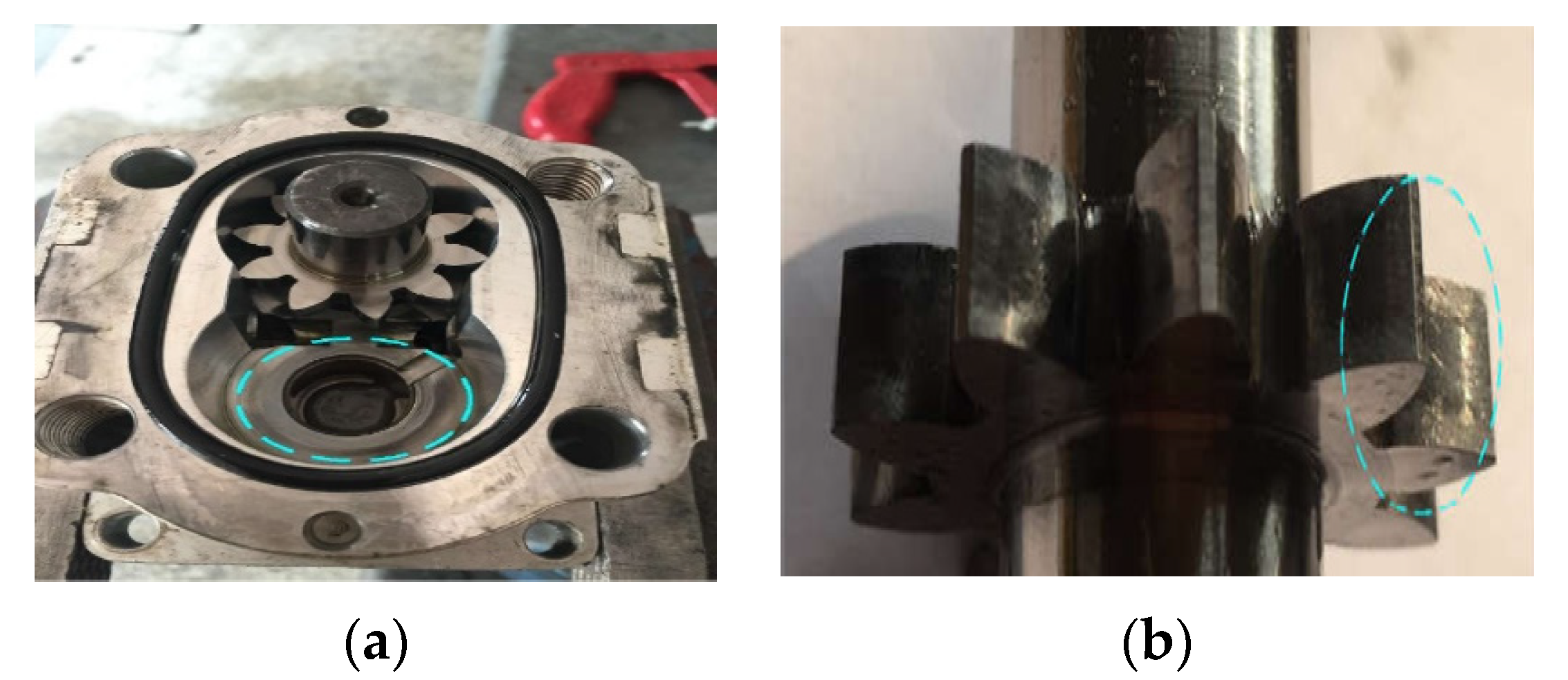
Determination of Test Data

The tested gear pump was disassembled after the test. It can be observed that the gear pump has obvious wear, as illustrated in Figure 6. The failure mechanism of the tested gear pump is wear, which leads to an increase in internal leakage and a decrease in volumetric efficiency. The flow degradation curve of the tested gear pump is shown in Figure 7. The output flow of the tested gear pump decreases significantly with the extension of running time. The flow rate of the gear pump decreases slowly in the early stage of operation and gradually accelerates in the later stage of operation until the failure threshold is reached. According to the wear condition and flow degradation curve, the experimental data are consistent with the degradation law of the initial wear stage and the stable wear stage.

In the experiment, each pump collected vibration signals in three directions: X, Y and Z. The vibration data of one pump were selected for analysis. Of the three directions, the Z direction has the largest amplitude. Considering that the end-face wear is the main wear form of the gear pump, the data in the Z direction were selected as the usage data in the vibration data. The vibration curve of one pump is shown in Figure 8.

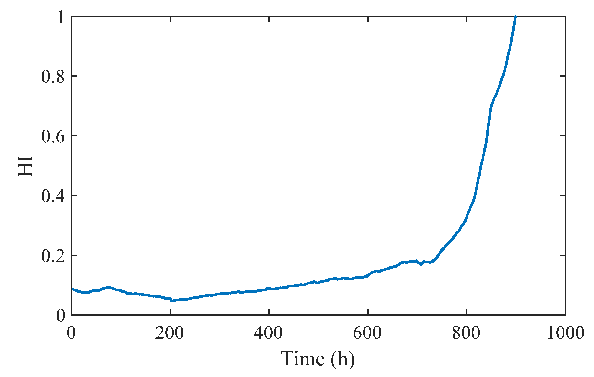
4. Modeling of Gear Pump Degradation State

This paper reflects the degradation status of gear pumps by constructing their HI. During the construction of HI, effective feature abstraction of the original data is required to explore its more in-depth representation. Multiple valid characteristics are combined to create a degradation curve reflecting the health of the gear pump. Figure 9 is the flow chart for obtaining the gear pump HI. Firstly, the original vibration signal is segmented, and the segmented data are directly input into the DCAE. In this paper, the one-dimensional convolutional kernel was selected to improve the coding network with respect to the characteristics of the vibration signal. During the experiment, it was found that the one-dimensional convolutional kernel enables efficient feature extraction of the vibration data as a time series. The decoding network consists of one-dimensional convolution layers and upsampling layers. The upsampling layer is represented as:

$$U_{n,l}^j=upsampling\left(X_{n,l}^j\right)$$

(11)

where $U_{n,m}^j$ is the output of the upsampling layer of the $j$-th object at the $n$-th data area of the $l$-th layer, and $X_{n,m}^j$ is the input of the $j$-th object at the $n$-th data area of the $l$-th layer.

The DCAE was trained to obtain a high-dimensional feature vector. SOM was used for feature dimensionality reduction. The output of the SOM network is the HI values of the gear pump.

The training steps for the DCAE and SOM network are illustrated using one of the gear pumps as an example.

Step 1: Based on the sampling frequency and the speed of the gear pump, the length of a single training sample is 2400; i.e., it contains 2400 individual vibration values.

Step 2: DCAE model training. In the encoder, there are six convolutional layers, and the number of convolutional kernels in every convolutional layer is: 32, 64, 128, 256, 64, 1. The maximum pooling layer is added after each convolution layer. In the decoder, there are six convolution layers, and the number of convolution kernels in every convolution layer is: 64, 256, 128, 64, 32, 1. The convolution kernel size of every convolution layer is 3 × 1. The size of the maximum pooling layer is 2 × 1. After each convolution layer, the ReLU function is used to activate it. The learning rate of the model is 0.001, and the optimizer is Adam. The batch size is 64. All of the test models mentioned in this paper were calculated by two GPUs, and the model was GeForce RTX 3090. The structure of the DCAE is indicated in Figure 10, where P1–P4 denotes the pooling layer, U1–U4 denotes the upsampling layer, and C1–C12 denotes the convolution layer.

Step 3: The vector of the hidden layer C6 in the DCAE is selected as the feature vector. The output of the C6 layer is used as the input to the SOM. In the SOM network, the number of nodes in the input layer is equal to the number of features in the C6 layer, both being 100.

Next are the training steps for the SOM network.

Step 3.1: The number of neurons in the topological layer in the SOM is defined as $r=5\sqrt{Y}$, and $Y$ is the input sample number.

Step 3.2: The input data for the SOM network at the $t$-th time is denoted by $x_t=\left\{x_{1t},x_{2t},\dots ,x_{100t}\right\}$. $x_{jt}$ is the $j$-th neuron at the $t$-th time point of the input layer, $j=1,2,\dots ,100$.

Step 3.3: The distance between neuron $d$ at the topological layer and input sample $x_t$ in the SOM network is represented by $d_t$.$\Vert x_t-w_l\Vert =\min \left\{d_t\right\}$. $w_l$ is the vector expression of the best-fitting neuron $l$. The vector of connection weights between every neuron in the topological layer and the neuron in the input layer to which it is attached is denoted as $w_{i^{\prime }}=\left\{w_{i^{\prime }1},w_{i^{\prime }2},\dots ,w_{i^{\prime }100}\right\}$; in the formula, $i^{\prime }=1,2,\dots ,d$. $i^{\prime }$ is the $i^{\prime }$-th neuron of the topological layer.

Step 3.4: Renew the linkage weights of best-fitting neurons $l$ and adjacent neurons with input layer neurons.

$$w_{i^{″}j}(n+1)=w_{i^{″}j}(n)+\eta (n)\cdot O_{i^{″},l}\cdot \left(x_{jt}-w_{i^{″}}(n)\right)$$

(12)

In the formula, $w_{i^{″}j}(n+1)$ is the connection weight of the $n+1$-th training of the input layer neuron $x_{jt}$ with the $i^{″}$-th neighborhood neuron in the topology layer.

$i^{″}$ is the $i^{″}$-th neighborhood neuron in the topological layer that surrounds the best-fitting neuron $l$. $\eta (n)$ is the augmentation function. $O_{i^{″},l}$ is the weight vector, which is represented by

$$O_{i^{″},l}=\exp \left(-S_{i^{″},l}^2/2{\sigma }^2\right)$$

(13)

where $S_{i^{″},l}^{}$ is the Euclidean distance between the $i^{″}$-th neighborhood neuron of the best-fitting neuron $l$. $\sigma$ is the criterion deviation of the distance between every neighborhood neuron and the best-fitting neuron $l$.

Step 3.5: At another point in time, a 100-dimensional sample is selected to provide the input layer to the SOM, and step 3 is repeated until each sample is provided to the SOM.

Step 3.6: Step 3.2 is repeated, and training is stopped when $n$ (training step $n=n+1$) equals the maximum number of training times $N$.

Step 3.7: The HI of the gear pump is calculated by Formula (14):

$$HI=MQE=\Vert x_t-w_l\Vert$$

(14)

where $MQE$ is the minimum quantization error.

Step 4: Validation and evaluation of DCAE.

In anticipation of a smoother HI curve, a sliding filtering process with a window width of 10 is executed on the obtained HI curve. The results are presented in Figure 11.

Three other methods were selected to compare with the proposed method, and the evaluation index was selected for quantitative analysis. The first method is named principal component analysis (PCA), and it extracts time-domain characteristics and frequency-domain characteristics from the data. These include skewness, center of gravity frequency, kurtosis, variance, margin index, peak value, root mean square frequency, waveform index, peak-to-peak value and frequency standard deviation. The 10 features derived were subjected to principal component analysis to obtain the state degradation curve of gear pumps. The algorithm in this paper was used as the second method [39], named stacked autoencoder (SAE). The third method was used in [40], named PAirwiSe CompArison Learning (PASCAL). The HI curves constructed based on the gear pump data with the four methods were compared. The HI curves constructed by the four methods are illustrated in Figure 12.

Two commonly used evaluation indicators, Monotonicity and Correlation, were selected to quantitatively analyze the four methods. Monotonicity measures the monotonic tendency of the HI curve to change, and Correlation indicates the tendency of the HI curve to degrade in relation to the time spent working.

The two evaluation indicators are expressed as follows:

$$V_{mon}=\left|\frac{NumofdF>0}{K-1}-\frac{NumofdF<0}{K-1}\right|$$

(15)

$$V_{corr}=\frac{\left|{\displaystyle \sum _{t=1}^T(K_t-\stackrel{\wedge }{K})}(l_t-\widehat{l})\right|}{\sqrt{{\displaystyle \sum _{t=1}^T{(K_t-\stackrel{\wedge }{K})}^2}{\displaystyle \sum _{t-1}^T{(l_t-\widehat{l})}^2}}}$$

(16)

In the formula, $K_t$ is the HI curve value of the $t$-th sample. $K$ is the total number of samples of the gear pump. dF is the difference between two contiguous objects in the HI curve.

$l_t$ is the sample number of the $t$-th sample. $\stackrel{\wedge }{K}$ and $\widehat{l}$ are the means of HI curve values and sample numbers, respectively.

Table 2. HI curve evaluation results.

Method		Pump1	Pump2	Pump3	Pump4
DCAE + SOM	Mon	0.21	0.22	0.17	0.15
	Corr	0.94	0.96	0.91	0.89
PCA	Mon	0.20	0.12	0.15	0.13
	Corr	0.75	0.76	0.79	0.73
SAE	Mon	0.17	0.11	0.12	0.09
	Corr	0.87	0.78	0.81	0.77
PASCAL	Mon	0.21	0.14	0.15	0.12
	Corr	0.90	0.84	0.87	0.85

presents the values of the evaluation indicators for the HI curves built by the method in this paper and the comparative methods described above. As shown in Figure 12, the proposed method is more sensitive to small early changes in the data. Combining Table 2 and Figure 12, the method proposed in this paper has the best monotonicity and trend. No human intervention is required during modeling, and feature self-extraction is achieved.

Parameter Selection

The core of the gear pump degradation state modeling scheme is based on one-dimensional convolution. In the degradation state modeling stage of the gear pump, the number of convolution kernels, the number of convolution layers and the size of convolution kernels have the most obvious influence on the training results. Several key factors are analyzed below. In the experimental stage, six network structures were designed for comparative analysis. The five network structures are shown in

Table 3. The different structures of DCAE.

Number	Number of Convolution Kernels	Number of Convolution Layers	Convolution Kernel Size
Structure 1	32-64-128-256-64-1-64-256-128-64-32-1	12	3 × 1
Structure 2	32-64-128-256-64-1-64-256-128-64-32-1	12	7 × 1
Structure 3	128-256-512-1024-512-1-512-1024-512-256-128-1	12	3 × 1
Structure 4	32-64-128-256-512-1024-512-256-1-256-512-1024-512-256-128-64-32-1	18	3 × 1
Structure 5	16-32-64-1-64-32-16-1	8	3 × 1

, and the parameters and parameter settings of each structure are consistent with those in Section 4. The network structure used in this paper is structure 1. Structure 6 is the same as structure 1, but the pooling layer of structure 6 adopts average pooling. Two evaluation indicators, Monotonicity and Correlation, were selected to analyze the HI constructed by each structure. The quantization results of each network structure are shown in

Table 4. Results of HI curve evaluation for six structural exercises.

Number	Gear Pump1		Gear Pump2		Gear Pump3		Gear Pump4
	Mon	Corr	Mon	Corr	Mon	Corr	Mon	Corr
Structure 1	0.21	0.94	0.22	0.96	0.17	0.91	0.15	0.89
Structure 2	0.14	0.85	0.17	0.85	0.13	0.87	0.12	0.75
Structure 3	0.19	0.91	0.17	0.92	0.15	0.89	0.15	0.89
Structure 4	0.05	0.35	0.01	0.33	0.03	0.34	0.02	0.35
Structure 5	0.08	0.45	0.09	0.55	0.10	0.59	0.11	0.60
Structure 6	0.19	0.90	0.18	0.92	0.14	0.89	0.11	0.85

.

By analyzing the experimental results, structure 1 has the best effect. Comparing structure 1 with structure 2, theoretically, a larger convolution kernel will have a larger perception field and receive more information. However, a large convolution kernel will result in an explosion of computation. When more convolutional layers are needed for complex data, the large convolution kernel will impact the performance of the model. A smaller convolution kernel size will reduce the calculation parameters. Structure 3 and structure 4 did not improve the training results but, on the contrary, led to a significant increase in training time. The original vibration data are noisy and vibratory, but as one-dimensional time-series data, their structure is not complicated. Massive convolutional kernels and convolutional layers do not lead to better training results. Especially in structure 4, the training result is worse, and the analysis of the loss function shows that overfitting occurs. The simple structure of structure 5 leads to incomplete learning results. Comparing structure 1 with structure 6, maximum pooling is slightly better than average pooling. Referring to the experience of other CNNs, in the experiment in this paper, maximum pooling will extract the most responsive and strongest part of the features and input it to the next stage. On the basis of the foregoing analysis, the structure of the DCAE in this paper is structure 1.

5. Prediction of RUL Based on Bi-LSTM

The scheme of mechanical pre-diagnosis usually consists of four processes: data collection, construction of health indicators, division of health stages and RUL prediction. The prediction of RUL can be directly based on original vibration data or based on health indicators. At present, there are mainly two ways to predict the RUL based on the health indicator: the trend extrapolation of the HI curve and direct mapping of the HI value to the RUL value. Despite the fact that both methods achieved good identification results, the acquisition of HI can be understood as feature extraction, and the recognition model does not directly identify it from the original data, which may result in different results from the actual situation, and also affects the recognition accuracy.

The remaining useful life prediction steps of the gear pump are shown in Figure 13. On the premise that the HI value of the gear pump has been obtained, the HI value is added as a label to each corresponding data. The labeled data are directly fed into the Bi-LSTM model for training. The output of Bi-LSTM is the predicted value of the RUL of the gear pump.

In intelligent diagnostic methods based on deep learning algorithms, there are two issues that have a significant impact on diagnostic results. The first is whether the network model matches the type of data. The second issue is the quality of the training data. Without considering the impact on data quality during data collection, the key issue that affects data quality in model training is whether the data are accurately labeled. At present, in supervised learning model training, training data need to be tagged. However, the common tagging methods used today are all about artificially adding labels to the data. In the process of adding labels to data, whether accurate labels can be added directly affects the quality of the data, thus affecting the accuracy of model training. In the data labeling phase, the labeled value is equivalent to a quantitative description of the degraded state of the gear pump. Currently, there are two primary approaches to labeling data during the training of life prediction models under supervised learning: the first method is illustrated in Figure 14a [41,42]. This method uses a linear function to label the data in the training set, which is defined as:

$$f\left(t_i\right)=-\left(\frac{1}{t_n}\ast t_i\right)+1$$

(17)

where $t_n$ is the complete life cycle, and $t_i$ is the prevailing time in the equipment life cycle.

The ordinate represents the RUL of the equipment under test. The linear function indicates that the degradation rate of the device is constant, which is obviously not in line with the actual situation.

The second method is illustrated in Figure 14b [43]. Its specific expression is

$$f\left(t_i\right)=\{\begin{array}{cc}1& t_i\le t_j\\ \left(\frac{1}{t_j-t_n}\right)\ast t_i+\left(\frac{t_n}{t_n-t_j}\right)& t_i>t_j\end{array}$$

(18)

where $t_j$ is the initial degradation time of the equipment. In Figure 14b, the health level remains unchanged until time point $t_j$. This method is not accurate enough. Firstly, in complex data, critical inflection points are difficult to find accurately; secondly, in the labeling method based on the piecewise function, the equipment degradation rate at different stages is also kept constant. In the early stage of equipment operation, slight changes in the equipment are ignored; during the accelerated degradation phase, the degradation rate of the equipment is clearly not constant. There are some problems in the models trained by these two methods. The RUL curve obtained by the model often fluctuates greatly, because the same label value is added to some data of different states. The training results of some models seem to be good, but they only accurately predict the label values, which are actually inconsistent with the real situation, leading to the poor generalization ability of the models.

The gear pump produces a large amount of data during its whole life cycle, and the data type is a one-dimensional continuous vibration signal, so the LSTM-based model was selected for RUL prediction. As degraded equipment, the gear pump has a strong correlation with the vibration data. LSTM can mine the information from the front to the back of the memory time series very well, but it fails to use the future information of the data, and the correlation analysis between the data is lacking. Therefore, this paper constructs a bidirectional long short-term memory (Bi-LSTM) network. The basic idea of Bi-LSTM is to add an additional layer of LSTM units, which is equivalent to re-calculating the input sequence inversely. The final result is a simple combination of the results of the two-layer LSTM network. Its structure is illustrated in Figure 15. The hidden layer state $H_t$ of Bi-LSTM at time $t$ is

$$\{\begin{array}{l}{H}_t=[{\overrightarrow{h}}_t,{\overleftarrow{h}}_t]\\ {\overrightarrow{h}}_t=\overrightarrow{\mathrm{LSTM}}(h_{t-1},x_t,c_{t-1}),t\in [1,T]\\ {\overleftarrow{h}}_t=\overleftarrow{\mathrm{LSTM}}(h_{t+1},x_t,c_{t+1}),t\in [1,T]\end{array}$$

(19)

In this equation, $x_t$ is the input at the $t$-th time, $h$ and $c$ are the hidden layer state and memory unit state, respectively, and $L$ is the sequence length.

In the actual experiment, it was found that the model learning ability of single-layer BI-LSTM was not strong. Therefore, the multi-layer Bi-LSTM was stacked to ensure that the constructed prediction model would have enough feature extraction ability and increase its nonlinear mapping ability. Figure 16 shows the network structure of the multi-layer Bi-LSTM prediction model. Starting from the second layer, the input of Bi-LSTM of each layer is the output of the hidden state of the time step of the previous layer; that is, the input of the Bi-LSTM unit at the $t$-th time of the $l$-th layer is $H_t^{l-1}=[{\overrightarrow{h}}_t^{l-1},{\overleftarrow{h}}_t^{l-1}]$, so the forward propagation process of multi-layer Bi-LSTM at time $t$ of the $l$-th layer is defined as follows:

$$\{\begin{array}{c}{f}_t^l=\sigma \left(W_f^l[h_{t-1}^l,H_t^{l-1}]+b_f^l\right)\\ i_t^l=\sigma \left(W_i^l[h_{t-1}^l,H_t^{l-1}]+b_i^l\right)\\ o_t^l=\sigma \left(W_o^l[h_{t-1}^l,H_t^{l-1}]+b_o^l\right)\end{array}$$

(20)

$$\{\begin{array}{l}{\tilde{C}}_t^l=\tanh \left(W_c^l[h_{t-1}^l,H_t^{l-1}]+b_c^l\right)\\ C_t^l=f_t^l\odot C_{t-1}^l+i_t^l\odot {\tilde{C}}_t^l\\ h_t^l=o_t^l\odot \tanh \left(C_t^l\right)\end{array}$$

(21)

In the formula, $f_t^l$, $i_t^l$ and $o_t^l$ are the forget gate, input gate and output gate of the Bi-LSTM unit at time $t$ in the $l$-th layer, respectively. $W_f^l$, $W_i^l$, $W_o^l$ and $W_c^l$ are the weight matrices of the $l$-th layer, and $b_f^l$, $b_i^l$, $b_o^l$ and $b_c^l$ are the bias vectors of the $l$-th layer.

The output of the last n-layer of Bi-LSTM at time $t$ is

$$y_t^n=\sigma \left(W_{h,y}{h}_t^n+b_{h,y}\right)$$

(22)

The output of the last time step in the last layer of Bi-LSTM is used as the input of the fully connected layer. The final RUL value is obtained from the output of the fully connected layer.

The following describes the RUL prediction process of gear pumps based on the multi-layer Bi-LSTM model.

Step 1: Building the HI of gear pumps.

Step 2: Dataset partitioning. There were four gear pumps in the experiment, and the training set and testing set were divided alternately. When the data of one gear pump were used as the testing set, the data of the other three gear pumps were used as the training set.

Step 3: Sample construction and labeling. The dataset of the original vibration signals is a one-dimensional sequence, but the input data dimension of the Bi-LSTM network requires [Batch Size, Time Steps, Feature Dims]. Batch Size is the number of batch samples, Time Steps is the time window size, and Feature Dims is the feature dimension. In the acquisition of HI, the sample length is 2400, so Time Steps is also set to 2400. The correspondence between each sample and the label value is maintained; that is, the label of the sample is the corresponding HI value.

Step 4: Multilayer Bi-LSTM model training. During model training, the batch size is 64; the selected loss function is the cross-entropy function; the chosen optimizer is Adam; the convolution kernel size of every convolution layer is 3 × 1; the size of the maximum pooling layer is 2 × 1; the learning rate is 0.001; and the maximum iteration number is 100. To avoid overfitting and to enhance the generalization ability of the model, the Dropout technique with a size of 0.5 is adopted after the first fully connected layer. At the same time, the model stops training when the loss function does not change significantly by using the early-stopping mechanism.

Step 5: Testing set validation.

Step 6: Evaluation of prediction algorithm.

In order to analyze the method proposed in this paper more concretely, three indicators were selected for quantitative analysis: (1) mean absolute error (MAE): MAE can accurately reflect the size of the forecast error; (2) root mean squared error (RMSE): RMSE can reflect the prediction accuracy of the model; (3) penalty score: the score given in the PHM2012 Data Challenge. The error percentage is represented in Formula (23), where $ActRU{L}_i$ and $PredRU{L}_i$ represent the actual and predicted remaining useful life values of the $i$-th predicted target. Taking into account that in the real world, the danger of equipment overprediction is less severe than the problem of underestimation, Formula (24) denotes the score of the $i$-th predicted target. Formula (25) is the score value of the ultimate prediction result, where N is the number of all test targets.

$$\%E_{r_i}=\frac{ActRU{L}_i-PredRU{L}_i}{ActRU{L}_i}\times 100\%$$

(23)

$$A_i=\{\begin{array}{ll}{\exp }^{-\ln (0.5)\cdot \left(\frac{E_{r_i}}{5}\right)}\hfill & \mathrm{if}{E}_{r_i}\le 0\hfill \\ {\exp }^{+\ln (0.5)\cdot \left(\frac{E_{r_i}}{20}\right)}\hfill & \mathrm{if}{E}_{r_i}>0\hfill \end{array}$$

(24)

$$\mathrm{Scor}e=\frac{1}{N}{\displaystyle \sum _{i=1}^N\left(A_i\right)}$$

(25)

The experiment found that in the training of the Bi-LSTM model, the most influential factor on the training results is the number of Bi-LSTM layers. For the purpose of investigating the effect of the number of Bi-LSTM layers on the prediction results, models with one to nine layers of Bi-LSTM were selected for tests, and the RMSE value of the test results was used as the evaluation index.

Figure 17 shows the experimental results. When the number of Bi-LSTM layers is 1, 2, 3 and 4, the RMSE value is larger. When the number of Bi-LSTM layers is 5, the prediction effect of the model is the best. However, after five layers, the RMSE value of the predicted results tends to increase with the number of layers. At this point, the curves of training loss and verification loss in the training process were observed. The loss continued to decline until convergence, but the verification loss tended to remain constant after rising. This indicates that the model at this time has overlearned the training set, leading to overfitting and thus a continuous decline in the model’s generalization ability. Additionally, with the increasing number of Bi-LSTM layers, the training time increased significantly. Therefore, based on the above factors, the number of Bi-LSTM layers in this model was set at 5. The life prediction results of one gear pump are shown in Figure 18. It can be appreciated that the predicted RUL values match the actual RUL curves better.

The major distinction between the proposed method and other methods is the change in the way that labels are added. The prediction performance of the proposed method was compared with that of models trained by other common labeling methods. The first method is the method in [28], and its labeling method is shown in Figure 14a, named Method 2 [28]. The second method is the method in [44], and its labeling method is shown in Figure 14b, named Method 3 [44]. The prediction effects of the models trained based on these two methods are shown in Figure 19.

Combining the analysis of the results in Figure 18 and Figure 19 shows that the prediction curve of Method 2 oscillates greatly around the true value. The reason should be that more data in the same state are marked with different label values, thus affecting the recognition effect. The prediction effect of Method 3 also produces large vibrations, especially in the stage of accelerated degradation of the gear pump. The predicted value of Method 3 is closer to the HI value constructed in this paper. Overall, the method proposed in this paper is the best.

Table 5. Evaluation results of models trained by three methods.

Method	Evaluation Index	Gear Pump1	Gear Pump2	Gear Pump3	Gear Pump4
HI–Method	MAE	0.025	0.026	0.019	0.033
	RMSE	0.012	0.028	0.037	0.027
	Score	0.601	0.624	0.599	0.581
Method 2	MAE	0.094	0.184	0.051	0.074
	RMSE	0.101	0.189	0.153	0.159
	Score	0.457	0.319	0.356	0.349
Method 3	MAE	0.074	0.052	0.049	0.089
	RMSE	0.103	0.098	0.089	0.074
	Score	0.462	0.474	0.431	0.399

shows that the HI–Method is superior to the other two methods in terms of the three performance indicators. Overall, the method proposed in this paper is the best.

6. Conclusions

A RUL prediction scheme for a gear pump is proposed, which combines equipment degradation state modeling with the RUL prediction method. Aiming at the situation of inadequate life data of the hydraulic pump, an accelerated life test scheme for the gear pump is proposed. The experimental data proved that the proposed scheme has good performance.

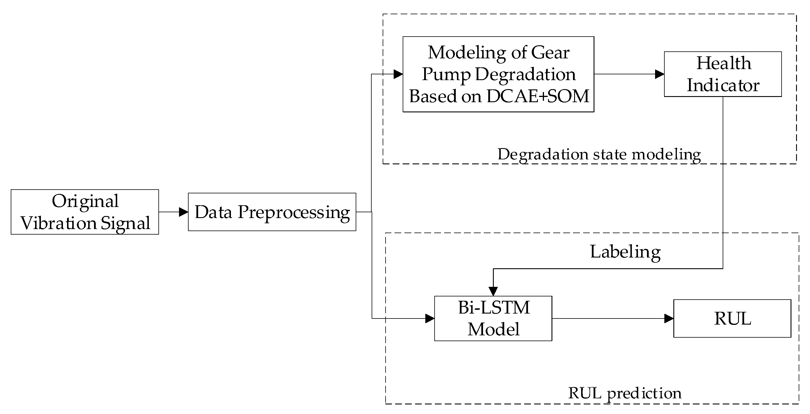
• A modeling method of gear pump degradation state combining a DCAE and SOM is proposed. The one-dimensional convolution kernel is used in the DCAE to improve the feature extraction capability of the model for one-dimensional vibration signals. The SOM network performs high-dimensional feature dimensionality reduction and obtains the HI of the gear pump. The entire modeling process is carried out in an unsupervised manner, reducing the dependence on manual labor.
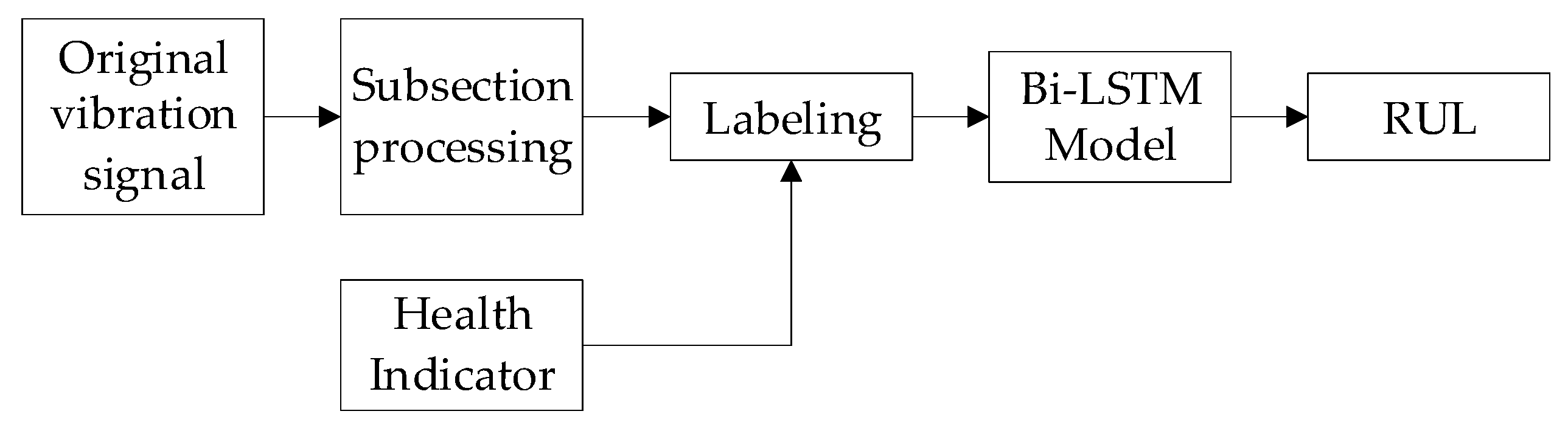
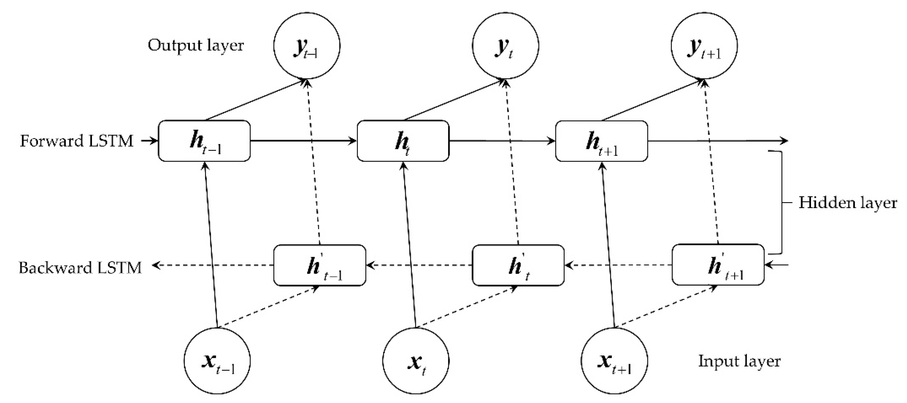
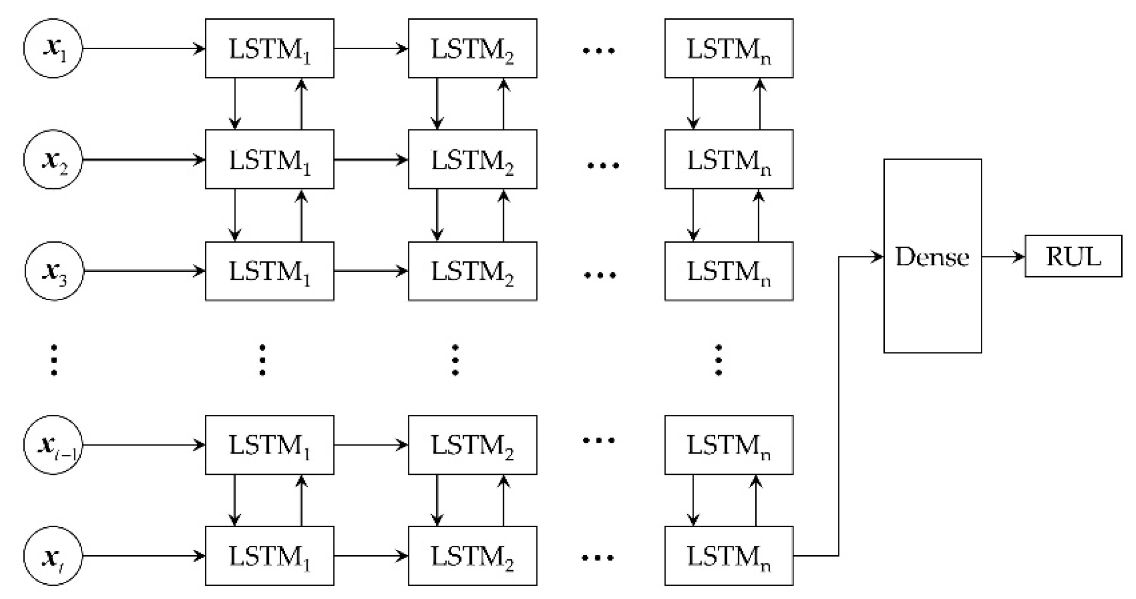
• A Bi-LSTM-based gear pump life prediction model is proposed. The model’s analysis of the associations between data is enhanced by the Bi-LSTM unit. The model is trained directly through the original data, and the output is the predicted value of RUL, realizing the end-to-end prediction. Especially in the process of data labeling, the HI value of the gear pump is used as the data label, instead of relying on manual labeling, which reduces the labeling error rate and dramatically enhances the quality of the training data. The evaluation indicators show that the presented method has superior prediction precision.
• The three central ideas of the proposed RUL scheme are one-dimensional convolution, the Bi-LSTM unit and the self-labeling of data. Thus, the scheme is very suitable for dealing with one-dimensional time-series data with strong correlation. The solution reduces the dependency on both manual and sophisticated signal processing algorithms and offers great flexibility and adaptability.

References

1. Lei, Y.; Li, N.; Guo, L.; Li, N.; Yan, T.; Lin, J. Machinery health prognostics: A systematic review from data acquisition to RUL prediction. Mech. Syst. Signal Process. 2018, 104, 799–834. [Google Scholar] [CrossRef]
2. Guo, S.; Chen, J.; Lu, Y.; Wang, Y.; Dong, H. Hydraulic piston pump in civil aircraft: Current status, future directions and critical technologies. Chin. J. Aeronaut. 2020, 33, 16–30. [Google Scholar] [CrossRef]
3. Lu, Y.; Huang, Z. A new hybrid model of sparsity empirical wavelet transform and adaptive dynamic least squares support vector machine for fault diagnosis of gear pump. Adv. Mech. Eng. 2020, 12, 1061–1068. [Google Scholar] [CrossRef]
4. Fausing Olesen, J.; Shaker, H.R. Predictive Maintenance for Pump Systems and Thermal Power Plants: State-of-the-Art Re-view, Trends and Challenges. Sensors 2020, 20, 2425. [Google Scholar] [CrossRef]
5. Cherniha, R.; Davydovych, V. A Mathematical Model for the COVID-19 Outbreak and Its Applications. Symmetry 2020, 12, 990. [Google Scholar] [CrossRef]
6. Al-Ayyoub, M.; Nuseir, A.; Alsmearat, K.; Jararweh, Y.; Gupta, B. Deep learning for Arabic NLP: A survey. J. Comput. Sci. 2018, 26, 522–531. [Google Scholar] [CrossRef]
7. Bhatt, D.; Patel, C.; Talsania, H.; Patel, J.; Vaghela, R.; Pandya, S.; Modi, K.; Ghayvat, H. CNN Variants for Computer Vision: History, Architecture, Application, Challenges and Future Scope. Electronics 2021, 10, 2470. [Google Scholar] [CrossRef]
8. Ma, X.; Hu, Y.; Wang, M.; Li, F.; Wang, Y. Degradation State Partition and Compound Fault Diagnosis of Rolling Bearing Based on Personalized Multilabel Learning. IEEE Trans. Instrum. Meas. 2021, 70, 3520711. [Google Scholar] [CrossRef]
9. Hamadache, M.; Jung, J.H.; Park, J.; Youn, B.D. A comprehensive review of artificial intelligence-based approaches for rolling element bearing PHM: Shallow and deep learning. JMST Adv. 2019, 1, 125–151. [Google Scholar] [CrossRef] [Green Version]
10. Ma, M.; Mao, Z. Deep-Convolution-Based LSTM Network for Remaining Useful Life Prediction. IEEE Trans. Ind. Inform. 2021, 17, 1658–1667. [Google Scholar] [CrossRef]
11. Zhao, Q.; Cheng, G.; Han, X.; Liang, D.; Wang, X. Fault Diagnosis of Main Pump in Converter Station Based on Deep Neural Network. Symmetry 2021, 13, 1284. [Google Scholar] [CrossRef]
12. Tang, S.; Yuan, S.; Zhu, Y. Deep Learning-Based Intelligent Fault Diagnosis Methods Toward Rotating Machinery. IEEE Access 2020, 8, 9335–9346. [Google Scholar] [CrossRef]
13. Zhao, R.; Yan, R.; Chen, Z.; Mao, K.; Wang, P.; Gao, R.X. Deep learning and its applications to machine health monitoring. Mech. Syst. Signal Process. 2019, 115, 213–237. [Google Scholar] [CrossRef]
14. Rezaeianjouybari, B.; Shang, Y. Deep learning for prognostics and health management: State of the art, challenges, and opportunities. Measurement 2020, 163, 107929. [Google Scholar] [CrossRef]
15. Guo, R.; Li, Y.; Zhao, L.; Zhao, J.; Gao, D. Remaining Useful Life Prediction Based on the Bayesian Regularized Radial Basis Function Neural Network for an External Gear Pump. IEEE Access 2020, 8, 107498–107509. [Google Scholar] [CrossRef]
16. Liang, X.; Duan, F.; Bennett, I.; Mba, D. A Sparse Autoencoder-Based Unsupervised Scheme for Pump Fault Detection and Isolation. Appl. Sci. 2020, 10, 6789. [Google Scholar] [CrossRef]
17. Li, Z.; Jiang, W.; Zhang, S.; Xue, D.; Zhang, S. Research on Prediction Method of Hydraulic Pump Remaining Useful Life Based on KPCA and JITL. Appl. Sci. 2021, 11, 9389. [Google Scholar] [CrossRef]
18. Tang, S.; Yuan, S.; Zhu, Y.; Li, G. An Integrated Deep Learning Method towards Fault Diagnosis of Hydraulic Axial Piston Pump. Sensors 2020, 20, 6576. [Google Scholar] [CrossRef]
19. Chen, H.; Xiong, Y.; Li, S.; Song, Z.; Hu, Z.; Liu, F. Multi-Sensor Data Driven with PARAFAC-IPSO-PNN for Identification of Mechanical Nonstationary Multi-Fault Mode. Machines 2022, 10, 155. [Google Scholar] [CrossRef]
20. Tang, H.; Fu, Z.; Huang, Y. A fault diagnosis method for loose slipper failure of piston pump in construction machinery under changing load. Appl. Acoust. 2021, 172, 107634. [Google Scholar] [CrossRef]
21. Lan, Y.; Hu, J.; Huang, J.; Niu, L.; Zeng, X.; Xiong, X.; Wu, B. Fault diagnosis on slipper abrasion of axial piston pump based on Extreme Learning Machine. Measurement 2018, 124, 378–385. [Google Scholar] [CrossRef]
22. Babikir, H.A.; Elaziz, M.A.; Elsheikh, A.H.; Showaib, E.A.; Elhadary, M.; Wu, D.; Liu, Y. Noise prediction of axial piston pump based on different valve materials using a modified artificial neural network model. Alex. Eng. J. 2019, 58, 1077–1087. [Google Scholar] [CrossRef]
23. Jiang, W.; Li, Z.; Li, J.; Zhu, Y.; Zhang, P. Study on a Fault Identification Method of the Hydraulic Pump Based on a Combi-nation of Voiceprint Characteristics and Extreme Learning Machine. Processes 2019, 7, 894. [Google Scholar] [CrossRef] [Green Version]
24. Zhu, Y.; Li, G.; Wang, R.; Tang, S.; Su, H.; Cao, K. Intelligent Fault Diagnosis of Hydraulic Piston Pump Based on Wavelet Analysis and Improved AlexNet. Sensors 2021, 21, 549. [Google Scholar] [CrossRef]
25. Li, X.; Zhang, W.; Ding, Q.; Sun, J.-Q. Intelligent rotating machinery fault diagnosis based on deep learning using data aug-mentation. J. Intell. Manuf. 2018, 31, 433–452. [Google Scholar] [CrossRef]
26. Ma, J.; Li, S.; Wang, X. Condition Monitoring of Rolling Bearing Based on Multi-Order FRFT and SSA-DBN. Symmetry 2022, 14, 320. [Google Scholar] [CrossRef]
27. Bhavsar, K.; Vakharia, V.; Chaudhari, R.; Vora, J.; Pimenov, D.Y.; Giasin, K. A Comparative Study to Predict Bearing Deg-radation Using Discrete Wavelet Transform (DWT), Tabular Generative Adversarial Networks (TGAN) and Machine Learning Models. Machines 2022, 10, 176. [Google Scholar] [CrossRef]
28. Zhan, Y.; Sun, S.; Li, X.; Wang, F. Combined Remaining Life Prediction of Multiple Bearings Based on EEMD-BILSTM. Symmetry 2022, 14, 251. [Google Scholar] [CrossRef]
29. Cao, Y.; Jia, M.; Ding, P.; Ding, Y. Transfer learning for remaining useful life prediction of multi-conditions bearings based on bidirectional-GRU network. Measurement 2021, 178, 109287. [Google Scholar] [CrossRef]
30. Pang, Y.; Jia, L.; Liu, Z. Discrete Cosine Transformation and Temporal Adjacent Convolutional Neural Network-Based Re-maining Useful Life Estimation of Bearings. Shock. Vib. 2020, 2020, 8240168. [Google Scholar]
31. Wang, R.; Shi, R.; Hu, X.; Shen, C.; Shi, H. Remaining Useful Life Prediction of Rolling Bearings Based on Multiscale Con-volutional Neural Network with Integrated Dilated Convolution Blocks. Shock. Vib. 2021, 2021, 8880041. [Google Scholar]
32. Fiebig, W.; Korzyb, M. Vibration and dynamic loads in external gear pumps. Arch. Civ. Mech. Eng. 2015, 15, 680–688. [Google Scholar] [CrossRef]
33. Al-Obaidi, A.R. Investigation of effect of pump rotational speed on performance and detection of cavitation within a cen-trifugal pump using vibration analysis. Heliyon 2019, 5, e01910. [Google Scholar] [CrossRef] [PubMed] [Green Version]
34. Liou, C.-Y.; Cheng, W.-C.; Liou, J.-W.; Liou, D.-R. Autoencoder for words. Neurocomputing 2014, 139, 84–96. [Google Scholar] [CrossRef]
35. Azarang, A.; Manoochehri, H.E.; Kehtarnavaz, N. Convolutional Autoencoder-Based Multispectral Image Fusion. IEEE Access 2019, 7, 35673–35683. [Google Scholar] [CrossRef]
36. Akhtar, N.; Ragavendran, U. Interpretation of intelligence in CNN-pooling processes: A methodological survey. Neural Comput. Appl. 2019, 32, 879–898. [Google Scholar] [CrossRef]
37. Wang, X.; Mao, D.; Li, X. Bearing fault diagnosis based on vibro-acoustic data fusion and 1D-CNN network. Measurement 2021, 173, 108518. [Google Scholar] [CrossRef]
38. Yu, Y.; Si, X.; Hu, C.; Zhang, J. A Review of Recurrent Neural Networks: LSTM Cells and Network Architectures. Neural Comput. 2019, 31, 1235–1270. [Google Scholar] [CrossRef]
39. Xu, F.; Huang, Z.; Yang, F.; Wang, D.; Tsui, K.L. Constructing a health indicator for roller bearings by using a stacked au-to-encoder with an exponential function to eliminate concussion. Appl. Soft Comput. 2020, 89, 106119. [Google Scholar] [CrossRef]
40. Cui, J.; Ren, L.; Wang, X.; Zhang, L. Pairwise comparison learning based bearing health quantitative modeling and its ap-plication in service life prediction. Future Gener. Comput. Syst. 2019, 97, 578–586. [Google Scholar] [CrossRef]
41. Deutsch, J.; He, D. Using Deep Learning-Based Approach to Predict Remaining Useful Life of Rotating Components. IEEE Trans. Syst. Man Cybern. Syst. 2018, 48, 11–20. [Google Scholar] [CrossRef]
42. Rai, A.; Kim, J.-M. A novel health indicator based on the Lyapunov exponent, a probabilistic self-organizing map, and the Gini-Simpson index for calculating the RUL of bearings. Measurement 2020, 164, 108002. [Google Scholar] [CrossRef]
43. Wang, H.; Peng, M.-J.; Miao, Z.; Liu, Y.-K.; Ayodeji, A.; Hao, C. Remaining useful life prediction techniques for electric valves based on convolution auto encoder and long short term memory. ISA Trans. 2021, 108, 333–342. [Google Scholar] [CrossRef] [PubMed]
44. Wu, J.; Hu, K.; Cheng, Y.; Zhu, H.; Shao, X.; Wang, Y. Data-driven remaining useful life prediction via multiple sensor sig-nals and deep long short-term memory neural network. ISA Trans. 2020, 97, 241–250. [Google Scholar] [CrossRef]
Figure 1. Gear pump RUL prediction scheme.
Symmetry 14 01111 g001
Figure 2. Classification of vibrations of gear pumps.
Symmetry 14 01111 g002
Figure 3. Basic structure of LSTM unit.
Symmetry 14 01111 g003
Figure 4. Schematic diagram of the constructed test bench: 1—gear pump; 2—torque speed meter; 3—motor; 4—safety valve; 5—pressure gauge; 6—magnetic exchange valve; 7—high-pressure filter; 8—high-pressure relief valve; 9—low-pressure relief valve; 10—flowmeter; 11—cooler; 12—air filter; 13—suction filter; 14—liquidometer; 15—oil tank.
Symmetry 14 01111 g004
Figure 5. Diagram of test bench equipment: (a) the front of the test bench; (b) the back of the test bench.
Symmetry 14 01111 g005
Figure 6. Wear and tear of gear pump: (a) side plate wear; (b) end-face wear of driving gear.
Symmetry 14 01111 g006
Figure 7. Gear pump output flow curve.
Symmetry 14 01111 g007
Figure 8. Gear pump vibration signal waveform.
Symmetry 14 01111 g008
Figure 9. The flow chart for obtaining gear pump HI.
Symmetry 14 01111 g009
Figure 10. DCAE structure diagram.
Symmetry 14 01111 g010
Figure 11. HI curve of the gear pump.
Symmetry 14 01111 g011
Figure 12. HI curves were constructed based on four methods.
Symmetry 14 01111 g012
Figure 13. The process of gear pump RUL prediction.
Symmetry 14 01111 g013
Figure 14. Two function curves describing the labeling method: (a) form of linear function; (b) form of segmentation function.
Symmetry 14 01111 g014
Figure 15. Bi-LSTM network expansion diagram.
Symmetry 14 01111 g015
Figure 16. Network structure of multi-layer Bi-LSTM prediction model.
Symmetry 14 01111 g016
Figure 17. Test results of the model with different Bi-LSTM layers.
Symmetry 14 01111 g017
Figure 18. Life prediction results of gear pump.
Symmetry 14 01111 g018
Figure 19. RUL prediction results of the two methods: (a) Method 2; (b) Method 3.
Symmetry 14 01111 g019