A Behavior-Simulated Spherical Fuzzy Extension of the Integrated Multi-Criteria Decision-Making Approach

Abstract

Since its inception in 1965, fuzzy sets have been developed for many years and are widely used in multi-criteria decision making (MCDM) problems. Recently, spherical fuzzy sets (SFS), one of the most recent fuzzy sets, have been applied to extend and reinforce MCDM methods. To contribute to this development, the aim of this study is to propose a novel SFS extension of the integrated MCDM method that takes into account the psychological behavior of decision makers. In the proposed approach, the evaluation criteria are first weighted by the spherical fuzzy Decision-Making Trial and Evaluation Laboratory (SF DEMATEL) method based on symmetrical linguistic comparison matrices. Another notable advantage of this process is determining the interrelationship between the evaluation criteria. In the next stage, the spherical fuzzy Interactive Multi-Criteria Decision-Making method in the Monte Carlo simulation environment (SF TODIM’MC) was applied to evaluate the alternatives. This method allows the process of evaluating alternatives to be performed continuously with different psychological behavioral parameters, which are considered as asymmetric information. As a result, the influence of the decision maker’s psychological behavior on the evaluation results is analyzed comprehensively. The robustness of the proposed approaches is verified through their application to prioritizing post-COVID-19 operational strategies in the Vietnam logistics sector. Numerical results have provided a cause-and-effect relationship between the negative effects of the pandemic and their weights. Furthermore, the results of prioritizing the operational strategies in the simulated environment provide rankings corresponding to different levels of risk aversion. Based on the results, the proposed spherical fuzzy approach is promising for expert-based decision-making problems under psycho-behavioral influence.

1. Introduction

In decision-making problems, crisp scales have difficulty in accurately expressing the judgments of decision-makers because of their intrinsic complexity and ambiguity. The psychological behavior of decision makers is considered as information asymmetry in the analysis process [1]. Uncertainty information is defined by a membership function by Zadeh, which marks the birth of the original fuzzy set [2]. In parallel with the development and evolution of multi-criteria decision-making methods, fuzzy sets have been studied and proposed continuously for decades [3]. Milestones in this development can be listed as type-2 fuzzy sets by Zadeh [4], intuitionistic fuzzy sets by Atanassov [5], interval type-2 fuzzy sets by Jerry et al. [6], Pythagorean fuzzy sets by Yager [7], neutrosophic fuzzy sets by Smarandache [8], hesitant fuzzy sets by Torra [9], and so on. Based on the synthesis of Pythagorean fuzzy sets and neutrosophic fuzzy sets, Kutlu Gündoğdu and Kutlu Gündoğdu introduced spherical fuzzy sets (SFS) in 2019 [10]. Accordingly, spherical fuzzy numbers (SFN) are defined using three parameters, including hesitancy, membership, and non-membership. As a result, decision makers are not only able to demonstrate their hesitancy but are also provided with a larger domain of preference for judgments. Moreover, according to prospect theory, the intrinsic complexity of decision makers is also reflected in other psychological behaviors [11]. Accordingly, decisions are influenced by three important principles: loss aversion, diminishing sensitivity, and reference dependence. The principle of loss aversion states that individuals’ sensitivity to losses is greater than to equal gains. The diminishing sensitivity principle indicates that individuals tend to be risk-seeking for losses and risk-averse for gains. Meanwhile, principle of loss aversion asserts individuals’ perceptions of gains and losses depend on a reference point. The application of these principles in the field of MCDM is marked by the initiation of the TODIM method (an acronym in Portuguese for Interactive Multi-Criteria Decision Making) by Gomes and Lima [12]. The TODIM method is a robust combination of aggregation and outranking approaches based on prospect theory. Applications of this approach have been found in many decision problems in both fuzzy and crisp environments [13,14,15]. Another emerging MCDM method is the Decision-Making Trial and Evaluation Laboratory method (DEMATEL). This method is an effective practical tool for identifying the potential interrelationships between criteria [16,17]. As discussed above, the SFN is advantageous in independently describing the hesitancy degrees in linguistic terms. The integration of these two methods, which have particular advantages, and spherical fuzzy sets can enhance the comprehensiveness of multi-criteria evaluations. Therefore, a theoretical research gap exists for the combination of DEMATEL and TODIM in spherical fuzzy environments for decision-making problems. Furthermore, the calculations in the original TODIM method are based on a given loss attenuation coefficient. Therefore, the big picture of the influence of this coefficient in the evaluation results cannot be described and analyzed. This motivates the need for an alternative approach where the effect of the loss attenuation coefficient is analyzed more generally.

Since the first cases were detected at the end of 2019, the rapid spread of the COVID-19 pandemic has affected many socio-economic areas on a global scale [18]. The pandemic has caused severe disruptions in global supply chains [19]. In the Asia-Pacific region, Vietnam is a country that has strong and comprehensive links with regional and global supply chains. The logistics activities play a significant role in the supply chain management. For the national economy, statistics show that logistics activities provided 3.5% of jobs and contributed 2.8% of total GDP in 2019 [20]. As a result, disruptions to global and regional supply chains will create significant difficulties for Vietnam’s economy. For the regional economy, the problems in Vietnam’s logistics activities have an indirect effect on the regional logistics activities because of Vietnam’s high connectivity. However, studies on post-COVID-19 operational strategies (OSs), which are based on the negative effects (NEs) of the pandemic on the logistics sector in Vietnam, are still lacking. This is a practical research gap that is expected to be narrowed by the results evaluated in this study.

The primary objective of this article is to propose a novel behavior-simulated spherical fuzzy extension of the integrated MCDM approach. The integrated approaches are constituted by the SF DEMATEL method and SF Monte Carlo TODIM (SF TODIM’MC) method. The proposed robust method does not only perform the two basic tasks of the MCDM methods, namely, determining the weights of the criteria and prioritizing the alternatives. In this study, the first combination of DEMATEL and TODIM also reinforces the integrated method with their two specific functions: the analysis of the interrelationship of the criteria and the influence of psychological behavior on decision makers. Besides, the TODIM’MC method, improved with a Monte Carlo simulation, allows a deeper analysis of the psychological behavior of the decision maker. Moreover, both the DEMATEL and TODIM’MC procedures are performed in a spherical fuzzy environment, one of the most recent fuzzy set theories. As a secondary research objective, the proposed approaches are applied to prioritize post-COVID-19 operational strategies for the logistics sector in Vietnam. In the first stage, the SF DEMATEL method is applied to analyze the negative effects of the pandemic. The purpose of this stage determines the weights of the NEs as well as the relationships between them. The second stage aimed to evaluate post-COVID operational strategies using the SF TODIM’MC method.

Accordingly, novel integrated approaches that combine SF DEMATEL and SF TODIM’MC are the theoretical and primary contributions of this study. The secondary contribution of this study is the results of the analysis of NEs and evaluation of post-COVID-19 OSs for Vietnam’s logistics sector. The in-depth insights into the NEs and potential performance of the OSs help managers determine the most appropriate strategic implementation roadmap for their businesses to survive, recover, and develop sustainably.

The remainder of this manuscript is structured as follows: Section 2 provides an overview of previous studies; Section 3 describes in detail the proposed novel approach; Section 4 presents the application of the novel approach to the case of Vietnam’s logistics sector; and Section 5 presents the conclusions and findings of this study.

2. Literature Review

Over the years, many approaches have been developed and proposed to multi-criteria decision-making (MCDM) problems, as shown in

Table 1. Integration of MCDM methods.

No.	Author	Year	Method	Fuzzy Sets	Other Factors
1	Youssef [33]	2020	BWM-TOPSIS	None
2	Bakir and Atalik [24]	2021	AHP-MARCOS	Triangular
3	Kannan et al. [28]	2021	BWM-VIKOR	None	Simulation
4	Liang et al. [27]	2021	BWM-VIKOR	Triangular
5	Liu et al. [14]	2021	TODIM-ELECTRE II	Hesitant
6	Mishra et al. [23]	2021	CoCoSo	Hesitant
7	Wang et al. [34]	2021	AHP-TOPSIS	Triangular	DEA models
8	Chai et al. [35]	2022	DEMATEL	Triangular
9	Seker and Aydin [26]	2022	SWARA-WASPAS	Intuitionistic
10	Wang et al. [13]	2022	BWM-TODIM	None	Simulation
11	Salimian et al. [36]	2022	VIKOR-MARCOS	Intuitionistic
12	Chodha et al. [25]	2022	TOPSIS-Entropy	None
13	Joshi et al. [37]	2022	TOPSIS	Hesitant
This study	Tai and Nhieu	2022	DEMATEL-TODIM’MC	Spherical	Monte Carlo Simulation

Note: SWARA—Stepwise Weight Assessment Ratio Analysis.

. A closer look at the review shows that primitive methods tend to be used in an integrative manner [21]. Most combinations of MCDM methods aim to individually perform the two tasks of weighting the criteria and prioritizing alternatives [22]. Methods based on pairwise comparisons, such as the Analytic Hierarchy Process (AHP) and the Best Worst Method (BWM), are often used to determine the weights of the criteria. Meanwhile, distance-based methods, such as the Evaluation based on Distance from Average Solution (EDAS) and the Technique for Order of Preference by Similarity to Ideal Solution (TOPSIS), or outranking methods, such as the Elimination Et Choice Translating Reality (ELECTRE), the Weighted Aggregated Sum Product Assessment (WASPAS), and the VIseKriterijumska Optimizacija I Kompromisno Resenje (VIKOR) are mainly used to prioritize alternatives [14,23,24,25,26,27,28]. On the other hand, novel methods inspired by breakthrough ideas are also introduced in this research area. In recent years, two methods have emerged: the Ordinal Priority Approach (OPA) by Ataei et al. and the Combined Compromise Solution (CoCoSo) by Morteza et al. [29,30]. Some MCDM methods are designed for special purposes beyond weighting criteria and prioritizing alternatives. The first remarkable case is the DEMATEL method. This method not only determines the weight of the criteria but also investigates the influence relationship between them [31]. The second remarkable case is the TODIM method. This method is designed to solve MCDM problems that consider the psychological behavior of decision makers. The TODIM method developed by Gomes and Lima is based on the prospect theory [12]. Prospect theory, introduced by Kahneman, is known as a descriptive theory for decision-making analysis under risk [11]. Three aspects of prospect theory applied in the TODIM method are diminishing sensitivity, loss aversion, and reference dependence. The calculations of the TODIM method have the participation of two factors, which represent the psychological behavior of the decision maker, the loss attenuation coefficient, and the reference criterion. In addition, extensions with fuzzy sets of MCDM methods are introduced with increasing popularity. Therefore, the evolution of fuzzy set types is roughly parallel with the development of MCDM methods. The most recent is the introduction of spherical fuzzy sets [32].

From the review of the different methods, these are the main points to conclude. The specific advantages of the DEMATEL and TODIM methods can be leveraged in an integrated approach. Furthermore, a Monte Carlo simulation can help the TODIM method provide a more comprehensive assessment of the psychological behavior of decision makers. Furthermore, an extended approach with Monte Carlo simulation and spherical fuzzy sets is believed to provide robust solutions and be able to comprehensively assess the psychological behavior of decision makers.

The literature review describes the previous and current attempts to address this issue. The COVID pandemic has caused all professions around the world to face new challenges. Therefore, during the outbreak of the pandemic as well as the present time, there have been many analytical studies on the effects of the global pandemic on the logistics sector. In 2020, a study on post-pandemic production strategies and challenges was conducted by Kumar et al. The results suggest that manufacturing companies should focus on reclamation and resource discovery. In addition, the authors emphasize the digitization of operations as a long-term recommendation to cope with future disruptions [38]. To assess the impacts of the pandemic on the food supply chain, Singh et al. developed a simulation model for the public distribution system. This model allows for to assessment of the health of the food supply chain under different disruption scenarios [39]. As a leading rice exporter, the stagnation in the logistics of Vietnam’s agricultural products not only adversely affects the country’s food security but also causes significant disruption to the regional food supply chain [40]. In 2020, Ani et al. introduced a combined method of system dynamics simulation (SDS) with multiple criteria decision aid (MCDA) determining the most appropriate operational strategy of the company. The SDS allows modeling of the current and possible interactions between the relevant elements of the system. Meanwhile, the MCDA determines the weights of the elements [41]. In addition, an AHP-based approach is proposed by Vieira et al. for designing operations at retail distribution centers based on the investigating the distribution strategy, the distribution operations, and internal activities [42]. Recently, Le and Nhieu proposed an integrated multi-criteria decision-making approach for the analysis of production strategies in the post-COVID era [43]. In 2021, Wang et al. developed a multi-objective mathematical optimization model to configure Vietnam’s agricultural supply chain with new uncertainties [44]. Several studies on the impact of the pandemic on logistics companies in Vietnam also have been conducted and published [45,46,47,48]. However, the strategic proposals operate mainly at the macro level. The relationship between the negative effects and mitigating potential of post-COVID-19 operational strategies for negative effects should be studied for specific cases rather than macroscopically. Therefore, this study aims at an analysis that is associated with the viewpoints and psychological behavior of logistics business managers.

3. Methodology

This study proposes a novel integrated approach consisting of two stages, as illustrated in Figure 1. The purpose of the first stage is to analyze the influence and relation of negative effects. This analysis is performed using the DEMATEL method in a spherical fuzzy environment. The calculations in the first stage also help determine the weight of the negative effects, which are used in the second stage. At Stage 2, this study evaluates operational strategies for manufacturing logistics networks using the spherical fuzzy TODIM method, which is enhanced by Monte Carlo simulation. According to prospect theory, decisions are influenced by the psychological behavior of the decision maker. The traditional TODIM method considered the effect of psychological behaviors as a loss attenuation coefficient. Accordingly, the evaluation results will change with different values of the loss attenuation coefficient. To evaluate operational strategies comprehensively and objectively, the calculations of the spherical fuzzy TODIM method in this study were performed in a Monte Carlo simulation environment. In each simulation replication, the value of the loss attenuation coefficient is randomly generated according to a given continuous uniform distribution. The evaluation results of the operational strategies are inductive from all simulation replications.

3.1. Spherical Fuzzy Sets

Since the applications of fuzzy sets to decision making were introduced by Bellman and Zadeh in 1970, the fuzzy sets’ extensions have been studied and introduced by many researchers [2,49]. As illustrated in Figure 2, fuzzy sets have evolved from ordinary fuzzy to other recent types over the years [4,5,7,8,9,10,50,51,52,53]. The recent extension of fuzzy sets, the spherical fuzzy sets (SFS), has found wide application in decision-making problems [32,54,55,56]. Spherical fuzzy membership functions consist of membership $\left(\alpha \right)$, non-membership $\left(\beta \right)$, and hesitancy $\left(\gamma \right)$ parameters. These parameters can be defined independently between 0 and 1.

The definition of SFS and its basic operators are presented as follows:

Definition 1.

Spherical fuzzy set ${\tilde{N}}_S$of the universe of discourse $T$is given by

$${\tilde{N}}_S=\left\{t,\left({\alpha }_{{\tilde{N}}_S}\left(t\right),{\beta }_{{\tilde{N}}_S}\left(t\right),{\gamma }_{{\tilde{N}}_S}\left(t\right)\right)|t\in T\right\}$$

(1)

where

$${\alpha }_{{\tilde{N}}_S}:T\to \left[0, 1\right], {\beta }_{{\tilde{N}}_S}:T\to \left[0, 1\right], {\gamma }_{{\tilde{N}}_S}:T\to \left[0, 1\right]$$

and

$$0\le {\alpha }_{{\tilde{N}}_S}^2\left(t\right)+{\beta }_{{\tilde{N}}_S}^2\left(t\right)+{\gamma }_{{\tilde{N}}_S}^2\left(t\right)\le 1 \forall t\in T$$

(2)

For each$t$, the numbers${\alpha }_{{\tilde{N}}_S}\left(t\right), {\beta }_{{\tilde{N}}_S}\left(t\right)$and${\gamma }_{{\tilde{N}}_S}\left(t\right)$are the degree of membership, non-membership, and hesitancy of$t$to${\tilde{N}}_S$, respectively.

Definition 2.

Let$T_1$and$T_2$be two universes and let${\tilde{N}}_S=\left({\alpha }_{{\tilde{N}}_S},{\beta }_{{\tilde{N}}_S},{\gamma }_{{\tilde{N}}_S}\right)$and${\tilde{M}}_S=\left({\alpha }_{{\tilde{M}}_S},{\beta }_{{\tilde{M}}_S},{\gamma }_{{\tilde{M}}_S}\right)$be two SFSs from the universe of discourse$T_1$and$T_2$. Basic operators are defined as follows:

Addition

$${\tilde{N}}_S\oplus {\tilde{M}}_S=\left\{\sqrt{{\alpha }_{{\tilde{N}}_S}^2+{\alpha }_{{\tilde{M}}_S}^2-{\alpha }_{{\tilde{N}}_S}^2{\alpha }_{{\tilde{M}}_S}^2},{\beta }_{{\tilde{N}}_S}{\beta }_{{\tilde{M}}_S},\sqrt{\left(1-{\alpha }_{{\tilde{M}}_S}^2\right){\gamma }_{{\tilde{N}}_S}^2+\left(1-{\alpha }_{{\tilde{N}}_S}^2\right){\gamma }_{{\tilde{M}}_S}^2-{\gamma }_{{\tilde{N}}_S}^2{\gamma }_{{\tilde{M}}_S}^2} \right\}$$

(3)

Multiplication

$${\tilde{N}}_S\otimes {\tilde{M}}_S=\left\{ {\alpha }_{{\tilde{N}}_S}{\alpha }_{{\tilde{M}}_S},\sqrt{{\beta }_{{\tilde{N}}_S}^2+{\beta }_{{\tilde{M}}_S}^2-{\beta }_{{\tilde{N}}_S}^2{\beta }_{{\tilde{M}}_S}^2},\sqrt{\left(1-{\beta }_{{\tilde{M}}_S}^2\right){\gamma }_{{\tilde{N}}_S}^2+\left(1-{\beta }_{{\tilde{N}}_S}^2\right){\gamma }_{{\tilde{M}}_S}^2-{\gamma }_{{\tilde{N}}_S}^2{\gamma }_{{\tilde{M}}_S}^2} \right\}$$

(4)

Multiplication by a scalar$(\mu >0)$

$$\mu {\tilde{N}}_S=\left\{\sqrt{1-{\left(1-{\alpha }_{{\tilde{N}}_S}^2\right)}^{\mu }},{\beta }_{{\tilde{N}}_S}^{\mu }, \sqrt{{\left(1-{\alpha }_{{\tilde{N}}_S}^2\right)}^{\mu }-{\left(1-{\alpha }_{{\tilde{N}}_S}^2-{\gamma }_{{\tilde{N}}_S}^2\right)}^{\mu }}\right\}$$

(5)

Power of${\tilde{N}}_S$ $(\mu >0)$

$${\tilde{N}}_S^{\mu }=\left\{{\alpha }_{{\tilde{N}}_S}^{\mu },\sqrt{1-{\left(1-{\beta }_{{\tilde{N}}_S}^2\right)}^{\mu }},\sqrt{{\left(1-{\beta }_{{\tilde{N}}_S}^2\right)}^{\mu }-{\left(1-{\beta }_{{\tilde{N}}_S}^2-{\gamma }_{{\tilde{N}}_S}^2\right)}^{\mu }}\right\}$$

(6)

Definition 3.

Consider the weight vector $w=\left(w_1,w_2,\dots ,w_n\right)$, where$0\le w_i\le 1$and ${{\displaystyle \sum }}_{i=1}^n{w}_i=1.$ Spherical weighted arithmetic mean (SWAM) and spherical weighted geometric mean (SWGM) are defined as follows:

$$\begin{gathered} SWA{M}_w\left({\tilde{N}}_{S1},{\tilde{N}}_{S2},\dots {\tilde{N}}_{Sn}\right)=w_1{\tilde{N}}_{S1}+w_2{\tilde{N}}_{S2}+\dots +w_n{\tilde{N}}_{Sn} \\ =\left\{\sqrt{1-{\displaystyle \prod }_{i=1}^n{\left(1-{\alpha }_{{\tilde{N}}_{Si}}^2\right)}^{w_i}},{\displaystyle \prod }_{i=1}^n{\beta }_{{\tilde{N}}_{Si}}^{w_i},\sqrt{{\displaystyle \prod }_{i=1}^n{\left(1-{\alpha }_{{\tilde{N}}_{Si}}^2\right)}^{w_i}-{\displaystyle \prod }_{i=1}^n{\left(1-{\alpha }_{{\tilde{N}}_{Si}}^2-{\gamma }_{{\tilde{N}}_{Si}}^2\right)}^{w_i}}\right\} \end{gathered}$$

(7)

$$\begin{gathered} SWG{M}_w\left({\tilde{N}}_{S1},{\tilde{N}}_{S2},\dots {\tilde{N}}_{Sn}\right)={\tilde{N}}_{S1}^{w_1}+{\tilde{N}}_{S2}^{w_2}+\dots +{\tilde{N}}_{Sn}^{w_n} \\ =\left\{{\displaystyle \prod }_{i=1}^n{\alpha }_{{\tilde{N}}_{Si}}^{w_i},\sqrt{1-{\displaystyle \prod }_{i=1}^n{\left(1-{\beta }_{{\tilde{N}}_{Si}}^2\right)}^{w_i}},\sqrt{{\displaystyle \prod }_{i=1}^n{\left(1-{\beta }_{{\tilde{N}}_{Si}}^2\right)}^{w_i}-{\displaystyle \prod }_{i=1}^n{\left(1-{\beta }_{{\tilde{N}}_{Si}}^2-{\gamma }_{{\tilde{N}}_{Si}}^2\right)}^{w_i}}\right\} \end{gathered}$$

(8)

Definition 4.

Let$T_1$and$T_2$be two universes and let ${\tilde{N}}_S=\left({\alpha }_{{\tilde{N}}_S},{\beta }_{{\tilde{N}}_S},{\gamma }_{{\tilde{N}}_S}\right)$and${\tilde{M}}_S=\left({\alpha }_{{\tilde{M}}_S},{\beta }_{{\tilde{M}}_S},{\gamma }_{{\tilde{M}}_S}\right)$be two SFSs from the universe of discourse $T_1$and$T_2$. The followings are valid under the condition$\mu$, ${\mu }_1$, ${\mu }_2>0$ [10].

$${\tilde{N}}_S\oplus {\tilde{M}}_S={\tilde{M}}_S\oplus {\tilde{N}}_S$$

(9)

$${\tilde{N}}_S\otimes {\tilde{M}}_S={\tilde{M}}_S\otimes {\tilde{N}}_S$$

(10)

$$\mu \left({\tilde{N}}_S\oplus {\tilde{M}}_S\right)=\mu {\tilde{N}}_S\oplus \mu {\tilde{M}}_S$$

(11)

$${\mu }_1{\tilde{N}}_S\oplus {\mu }_2{\tilde{N}}_S=\left({\mu }_1+{\mu }_2\right){\tilde{N}}_S$$

(12)

$${\left({\tilde{N}}_S\otimes {\tilde{M}}_S\right)}^{\mu }={\tilde{N}}_S^{\mu }\otimes {\tilde{M}}_S^{\mu }$$

(13)

$${\tilde{N}}_S^{{\mu }_1}\otimes {\tilde{N}}_S^{{\mu }_2}={\tilde{N}}_S^{{\mu }_1+{\mu }_2}$$

(14)

Definition 5.

Let$T$be the universal set and$t_i\in T; \forall i=1, 2, \dots , n$then${\tilde{N}}_S=\left({\alpha }_{{\tilde{N}}_S}\left(t_i\right),{\beta }_{{\tilde{N}}_S}\left(t_i\right),{\gamma }_{{\tilde{N}}_S}\left(t_i\right)\right)$and${\tilde{M}}_S=\left({\alpha }_{{\tilde{M}}_S}\left(t_i\right),{\beta }_{{\tilde{M}}_S}\left(t_i\right),{\gamma }_{{\tilde{M}}_S}\left(t_i\right)\right)$be two spherical fuzzy sets. The normalized Minkowski distance$MD\left({\tilde{N}}_S,{\tilde{M}}_S\right)$is defined under the condition$\rho \ge 1$as follows [57]:

$$MD\left({\tilde{N}}_S,{\tilde{M}}_S\right)=\sqrt[\rho ]{\frac{1}{2n}{\displaystyle \sum }_{i=1}^n\left({\left|{\alpha }_{{\tilde{N}}_S}^2\left(t_i\right)-{\alpha }_{{\tilde{M}}_S}^2\left(t_i\right)\right|}^{\rho }+{\left|{\beta }_{{\tilde{N}}_S}^2\left(t_i\right)-{\beta }_{{\tilde{M}}_S}^2\left(t_i\right)\right|}^{\rho }+{\left|{\gamma }_{{\tilde{N}}_S}^2\left(t_i\right)-{\gamma }_{{\tilde{M}}_S}^2\left(t_i\right)\right|}^{\rho }\right) }$$

(15)

If$\rho =2$, the Minkowski distance will turn into Euclidean distance

$$ED\left({\tilde{N}}_S,{\tilde{M}}_S\right)=\sqrt{\frac{1}{2n}{\displaystyle \sum }_{i=1}^n\left({\left|{\alpha }_{{\tilde{N}}_S}^2\left(t_i\right)-{\alpha }_{{\tilde{M}}_S}^2\left(t_i\right)\right|}^2+{\left|{\beta }_{{\tilde{N}}_S}^2\left(t_i\right)-{\beta }_{{\tilde{M}}_S}^2\left(t_i\right)\right|}^2+{\left|{\gamma }_{{\tilde{N}}_S}^2\left(t_i\right)-{\gamma }_{{\tilde{M}}_S}^2\left(t_i\right)\right|}^2\right)}$$

(16)

If$\rho =1$, the Minkowski distance will turn into Hamming distance

$$HD\left({\tilde{N}}_S,{\tilde{M}}_S\right)=\frac{1}{2n}{\displaystyle \sum }_{i=1}^n\left(\left|{\alpha }_{{\tilde{N}}_S}^2\left(t_i\right)-{\alpha }_{{\tilde{M}}_S}^2\left(t_i\right)\right|+\left|{\beta }_{{\tilde{N}}_S}^2\left(t_i\right)-{\beta }_{{\tilde{M}}_S}^2\left(t_i\right)\right|+\left|{\gamma }_{{\tilde{N}}_S}^2\left(t_i\right)-{\gamma }_{{\tilde{M}}_S}^2\left(t_i\right)\right|\right)$$

(17)

Definition 6.

For defuzzification and comparison, the score function and accuracy function of SFS are defined as follows:

$$\begin{gathered} {\tilde{N}}_S<{\tilde{M}}_S if and only if \\ i. Score\left({\tilde{N}}_S\right)<Score\left({\tilde{M}}_S\right) or \\ ii. Score\left({\tilde{N}}_S\right)=Score\left({\tilde{M}}_S\right) and Accuracy\left({\tilde{N}}_S\right)<Accuracy\left({\tilde{M}}_S\right) \end{gathered}$$

(18)

where

$$Score\left({\tilde{N}}_S\right)={\left({\alpha }_{{\tilde{N}}_S}-{\gamma }_{{\tilde{N}}_S}\right)}^2+{\left({\beta }_{{\tilde{N}}_S}-{\gamma }_{{\tilde{N}}_S}\right)}^2$$

(19)

$$Accuracy\left({\tilde{N}}_S\right)={\alpha }_{{\tilde{N}}_S}^2+{\beta }_{{\tilde{N}}_S}^2+{\gamma }_{{\tilde{N}}_S}^2$$

(20)

3.2. The Extended Spherical Fuzzy DEMATEL (SF DEMATEL)

The DEMATEL technique was devised by Fontela and Gabus in 1974 to analyze the influence relationships of components in an intricate system [58]. The original idea of the DEMATEL technique was to evaluate the interrelationships among all the variables, attributes, factors, or criteria of a complex system. This technique is widely applied to assessment implementation, policy development, and strategy formulation in a lot of areas, such as decision sciences, management, engineering, computer science, and social sciences. Extensions of the DEMATEL method with fuzzy sets are widely studied and introduced in research related to decision making [31]. The extended spherical fuzzy DEMATEL technique is summarized in the following steps:

Step 1. Criteria and decision-makers identification

First, a group of experts or decision makers $\left(k=1\dots K\right)$ is defined for the problem to be analyzed. Next, the criteria $\left(j=1\dots J\right)$ are clarified based on the references or opinions of the decision makers. In this study, the negative effects of the pandemic are considered as the criteria of a multi-criteria decision problem.

Step 2. Expert prioritizing

Because the expertise, experience, and knowledge of the decision makers are different, the weights of the decision makers should be determined. The SFNs that represent the expertise of the experts are provided by the higher-level decision maker. For example, the authors of this study will perform a linguistics assessment for experts based on their expertise, such as qualifications, years of experience, and number of publications cited, and so on. Assume that SF ${\tilde{N}}_k=\left({\alpha }_k,{\beta }_k,{\gamma }_k\right)$ represents the expertise of the $k$th decision maker. The weight coefficient of the $k$th decision maker is defined as Equation (21) [59].

$${\sigma }_k=\frac{1-\sqrt{\left(\left(1-{\alpha }_k^2\right)+{\beta }_k^2+{\gamma }_k^2\right)/3}}{{{\displaystyle \sum }}_k\left(1-\sqrt{\left(\left(1-{\alpha }_k^2\right)+{\beta }_k^2+F{\gamma }_k^2\right)/3}\right)}$$

(21)

where ${{\displaystyle \sum }}_{k=1}^K{\sigma }_k=1$ and $0\le {\alpha }_k^2+{\beta }_k^2+{\gamma }_k^2\le 1$

Step 3. The direct influence evaluation matrix construction

Pairwise linguistics comparisons of the potential influence between the criteria are provided by the decision makers. The $k$th decision maker’s linguistic evaluation of the potential influence of criterion $j$ on criterion $l$ is denoted as $q_{jl}^k$, where $j, l=1\dots J, k=1\dots K$. To perform the quantitative analysis, the linguistic pairwise comparisons are converted to SF numbers according to the relationships as shown in

Table 2. Linguistic terms and SF numbers relationship in SF DEMETAL [32].

Influence Degree	Linguistic Term	Spherical Fuzzy Parameters
		$\mathit{\alpha }$	$\mathit{\beta }$	$\mathit{\gamma }$
No influence	NI	0	0.3	0.15
Week influence	WI	0.35	0.25	0.25
Moderate influence	MI	0.60	0.2	0.35
Strong influence	SI	0.85	0.15	0.45

. The $k$th decision maker’s SF evaluation of the potential influence of criterion $j$ on criterion $l$ is denoted as ${\tilde{d}}_{jl}^k=\left({\alpha }_{jl}^k,{\beta }_{jl}^k,{\gamma }_{jl}^k\right)$. The SF direct influence evaluation matrix of the $k\mathrm{th}$ decision maker is shown by $D^k={\left[{\tilde{d}}_{jl}^k\right]}_{JxJ}={\left[\left({\alpha }_{jl}^k,{\beta }_{jl}^k,{\gamma }_{jl}^k\right)\right]}_{JxJ}$.

Step 4. The aggregated direct influence matrix construction

Based on the decision makers’ weight coefficient (${\sigma }_k$), the spherical weight arithmetic mean (SWAM) is applied to aggregate the direct influence evaluation matrices of the decision makers according to Equation (7). The aggregated direct influence matrix is represented as Equation (22).

$$D^{*}={[{\tilde{d}}_{jl}^{*}]}_{JxJ}=\left[\begin{array}{cc}\begin{array}{cc}\left({\alpha }_{11}^{*},{\beta }_{11}^{*},{\gamma }_{11}^{*}\right)& \left({\alpha }_{12}^{*},{\beta }_{12}^{*},{\gamma }_{12}^{*}\right)\\ \left({\alpha }_{21}^{*},{\beta }_{21}^{*},{\gamma }_{21}^{*}\right)& \left({\alpha }_{22}^{*},{\beta }_{22}^{*},{\gamma }_{22}^{*}\right)\end{array}& \begin{array}{cc}\cdots & \left({\alpha }_{1J}^{*},{\beta }_{1J}^{*},{\gamma }_{1J}^{*}\right)\\ \cdots & \left({\alpha }_{2J}^{*},{\beta }_{2J}^{*},{\gamma }_{2J}^{*}\right)\end{array}\\ \begin{array}{cc}⋮& ⋮\\ \left({\alpha }_{J1}^{*},{\beta }_{J1}^{*},{\gamma }_{J1}^{*}\right)& \left({\alpha }_{J2}^{*},{\beta }_{J2}^{*},{\gamma }_{J2}^{*}\right)\end{array}& \begin{array}{cc}\ddots & ⋮\\ \cdots & \left({\alpha }_{JJ}^{*},{\beta }_{JJ}^{*},{\gamma }_{JJ}^{*}\right)\end{array}\end{array}\right]$$

(22)

where

$${\tilde{d}}_{jl}^{*}=SWA{M}_{{\sigma }_k}\left({\tilde{d}}_{jl}^1,{\tilde{d}}_{jl}^2,\dots {\tilde{d}}_{jl}^k\right)={\sigma }_1{\tilde{d}}_{jl}^1+{\sigma }_2{\tilde{d}}_{jl}^2+\dots +{\sigma }_k{\tilde{d}}_{jl}^k$$

Step 5. The initial direct influence submatrices construction

For normalization, the aggregated direct influence matrix is divided into three submatrices corresponding to each SF parameter. These matrices are represented as Equation (23). The normalization process is performed according to Equations (24)–(26).

$$D^{\alpha }=\left[\begin{array}{cc}\begin{array}{cc}{\alpha }_{11}^{*}& {\alpha }_{12}^{*}\\ {\alpha }_{21}^{*}& {\alpha }_{22}^{*}\end{array}& \begin{array}{cc}\cdots & {\alpha }_{1J}^{*}\\ \cdots & {\alpha }_{2J}^{*}\end{array}\\ \begin{array}{cc}⋮& ⋮\\ {\alpha }_{J1}^{*}& {\alpha }_{J2}^{*}\end{array}& \begin{array}{cc}\ddots & ⋮\\ \cdots & {\alpha }_{JJ}^{*}\end{array}\end{array}\right],D^{\beta }=\left[\begin{array}{cc}\begin{array}{cc}{\beta }_{11}^{*}& {\beta }_{12}^{*}\\ {\beta }_{21}^{*}& {\beta }_{22}^{*}\end{array}& \begin{array}{cc}\cdots & {\beta }_{1J}^{*}\\ \cdots & {\beta }_{2J}^{*}\end{array}\\ \begin{array}{cc}⋮& ⋮\\ {\beta }_{J1}^{*}& {\beta }_{J2}^{*}\end{array}& \begin{array}{cc}\ddots & ⋮\\ \cdots & {\beta }_{JJ}^{*}\end{array}\end{array}\right],D^{\gamma }=\left[\begin{array}{cc}\begin{array}{cc}{\gamma }_{11}^{*}& {\gamma }_{12}^{*}\\ {\gamma }_{21}^{*}& {\gamma }_{22}^{*}\end{array}& \begin{array}{cc}\cdots & {\gamma }_{1J}^{*}\\ \cdots & {\gamma }_{2J}^{*}\end{array}\\ \begin{array}{cc}⋮& ⋮\\ ,{\gamma }_{J1}^{*}& {\gamma }_{J2}^{*}\end{array}& \begin{array}{cc}\ddots & ⋮\\ \cdots & {\gamma }_{JJ}^{*}\end{array}\end{array}\right]$$

(23)

$$Y^{\alpha }=s^{\alpha }\times D^{\alpha }, \mathrm{where} s^{\alpha }=min\left(\frac{1}{\underset{j}{\max }{{\displaystyle \sum }}_{l=1}^J{\alpha }_{il}^{*}},\frac{1}{\underset{l}{\max }{{\displaystyle \sum }}_{j=1}^J{\alpha }_{il}^{*}}\right)$$

(24)

$$Y^{\beta }=s^{\beta }\times D^{\beta }, \mathrm{where}{s}^{\beta }=min\left(\frac{1}{\underset{j}{\max }{{\displaystyle \sum }}_{l=1}^J{\beta }_{il}^{*}},\frac{1}{\underset{l}{\max }{{\displaystyle \sum }}_{j=1}^J{\beta }_{il}^{*}}\right)$$

(25)

$$Y^{\gamma }=s^{\gamma }\times D^{\gamma }, \mathrm{where}{s}^{\gamma }=min\left(\frac{1}{\underset{j}{\max }{{\displaystyle \sum }}_{l=1}^J{\gamma }_{il}^{*}},\frac{1}{\underset{l}{\max }{{\displaystyle \sum }}_{j=1}^J{\gamma }_{il}^{*}}\right)$$

(26)

Step 6. The total influence matrix determination

The total influence is calculated by adding the direct effects to the indirect effects. In this step, the initial direct influence submatrices are converted into total influence submatrices according to the Equations (27)–(29) [31]. However, the conversion process may return non-fuzzy results in some cases. Therefore, to make them convenient to the nature of the SFS, Euclidean normalization can be used to adjust the results.

$$X^{\alpha }=Y^{\alpha }+Y^{{\alpha }^{\prime }}=Y^{\alpha }{\left(I-Y^{\alpha }\right)}^{-1}=\left[\begin{array}{cc}\begin{array}{cc}{\alpha }_{11}^{**}& {\alpha }_{12}^{**}\\ {\alpha }_{21}^{**}& {\alpha }_{22}^{**}\end{array}& \begin{array}{cc}\cdots & {\alpha }_{1J}^{**}\\ \cdots & {\alpha }_{2J}^{**}\end{array}\\ \begin{array}{cc}⋮& ⋮\\ {\alpha }_{J1}^{**}& {\alpha }_{J2}^{**}\end{array}& \begin{array}{cc}\ddots & ⋮\\ \cdots & {\alpha }_{JJ}^{**}\end{array}\end{array}\right]$$

(27)

$$X^{\beta }=Y^{\beta }+Y^{{\beta }^{\prime }}=Y^{\beta }{\left(I-Y^{\beta }\right)}^{-1}=\left[\begin{array}{cc}\begin{array}{cc}{\beta }_{11}^{**}& {\beta }_{12}^{**}\\ {\beta }_{21}^{**}& {\beta }_{22}^{**}\end{array}& \begin{array}{cc}\cdots & {\beta }_{1J}^{**}\\ \cdots & {\beta }_{2J}^{**}\end{array}\\ \begin{array}{cc}⋮& ⋮\\ {\beta }_{J1}^{**}& {\beta }_{J2}^{**}\end{array}& \begin{array}{cc}\ddots & ⋮\\ \cdots & {\beta }_{JJ}^{**}\end{array}\end{array}\right]$$

(28)

$$X^{\gamma }=Y^{\gamma }+Y^{{\gamma }^{\prime }}=Y^{\gamma }{\left(I-Y^{\gamma }\right)}^{-1}=\left[\begin{array}{cc}\begin{array}{cc}{\gamma }_{11}^{**}& {\gamma }_{12}^{**}\\ {\gamma }_{21}^{**}& {\gamma }_{22}^{**}\end{array}& \begin{array}{cc}\cdots & {\gamma }_{1J}^{**}\\ \cdots & {\gamma }_{2J}^{**}\end{array}\\ \begin{array}{cc}⋮& ⋮\\ {\gamma }_{J1}^{**}& {\gamma }_{J2}^{**}\end{array}& \begin{array}{cc}\ddots & ⋮\\ \cdots & {\gamma }_{JJ}^{**}\end{array}\end{array}\right]$$

(29)

The total influence matrix is constructed by recombining the submatrices, which is represented as Equation (30).

$$X^{*}={[{\tilde{x}}_{il}]}_{JxJ}=\left[\begin{array}{cc}\begin{array}{cc}\left({\alpha }_{11}^{**},{\beta }_{11}^{**},{\gamma }_{11}^{**}\right)& \left({\alpha }_{12}^{**},{\beta }_{12}^{**},{\gamma }_{12}^{**}\right)\\ \left({\alpha }_{21}^{**},{\beta }_{21}^{**},{\gamma }_{21}^{**}\right)& \left({\alpha }_{22}^{**},{\beta }_{22}^{**},{\gamma }_{22}^{**}\right)\end{array}& \begin{array}{cc}\cdots & \left({\alpha }_{1J}^{**},{\beta }_{1J}^{**},{\gamma }_{1J}^{**}\right)\\ \cdots & \left({\alpha }_{2J}^{**},{\beta }_{2J}^{**},{\gamma }_{2J}^{**}\right)\end{array}\\ \begin{array}{cc}⋮& ⋮\\ \left({\alpha }_{J1}^{**},{\beta }_{J1}^{**},{\gamma }_{J1}^{**}\right)& \left({\alpha }_{J2}^{**},{\beta }_{J2}^{**},{\gamma }_{J2}^{**}\right)\end{array}& \begin{array}{cc}\ddots & ⋮\\ \cdots & \left({\alpha }_{JJ}^{**},{\beta }_{JJ}^{**},{\gamma }_{JJ}^{**}\right)\end{array}\end{array}\right]$$

(30)

Step 7. Spherical fuzzy row and column sums calculation

By utilizing the addition operator as shown in Equation (3), the spherical fuzzy row sum $\left({\tilde{r}}_j\right)$ and column sum $\left({\tilde{c}}_l\right)$ of the total influence matrix are calculated according to Equations (31) and (32).

$${\tilde{r}}_j={{\displaystyle \sum }}_{l=1}^J\left({\alpha }_{jl}^{**},{\beta }_{jl}^{**},{\gamma }_{jl}^{**}\right) j=1\dots J$$

(31)

$${\tilde{c}}_l={{\displaystyle \sum }}_{j=1}^J\left({\alpha }_{jl}^{**},{\beta }_{jl}^{**},{\gamma }_{jl}^{**}\right) l=1\dots J$$

(32)

Step 8. Prominence, relation, and weight values calculation

To determine the degree of prominence $\left(r+c\right)$ and relation $\left(r-c\right)$, defuzzification for the spherical fuzzy row sum $\left({\tilde{r}}_j\right)$ and column sum $\left({\tilde{c}}_l\right)$ is performed according to Equation (13). Then, the weights of the criteria are determined according to Equation (33).

$$w_j=\frac{r_j+c_j}{{{\displaystyle \sum }}_{j=1}^J\left(r_j+c_j\right)} j=1\dots J$$

(33)

Step 9. Drawing network relations map (NRM)

The network relations map is formed by horizontal and vertical axes, named “Prominence” and “Relation”, respectively. The relation $\left(r-c\right)$ illustrates the net effect that is contributed by the criterion. The $j\mathrm{th}$ criterion can be grouped into the cause group if $\left(r_j-c_j\right)$ is positive. Conversely, if $\left(r_j-c_j\right)$ is negative, the $j\mathrm{th}$ criterion is influenced by the other criteria. Then, it can be grouped into the effect group. The prominence $\left(r+c\right)$ represents the strength of influence that is received or given by the criterion. By calculating the mean of prominence $\left(r+c\right)$, the NRM can be divided into four quadrants, as illustrated in Figure 3.

3.3. The Extended Spherical Fuzzy TODIM with Monte Carlo Simulation (SF TODIM’MC)

The TODIM is a multi-criteria decision-making method that combines the properties of outranking approaches and aggregation approaches. Since the TODIM method was developed on the basis of prospect theory, it allows the psychological behavior of decision makers to be taken into account in the evaluation process. Moreover, the TODIM method has been universally integrated with fuzzy sets in recent studies. Extensions of the TODIM method with triangular fuzzy sets, Pythagorean fuzzy sets, and hesitant fuzzy sets have been found [60,61,62]. In this study, the combination of the TODIM method and spherical fuzzy sets is introduced. Considering the decision maker’s psychological behavior, the Monte Carlo simulation process has been integrated with the SF TODIM method. The procedure of the novel proposed method, named the Extended spherical fuzzy TODIM with Monte Carlo simulation (SF TODIM’MC), includes the following steps:

Step 1. The individual linguistic performance evaluations

Experts or decision makers $\left(k=1\dots K\right)$ are asked to provide linguistic performance evaluation alternatives $\left(i=1\dots I\right)$ according to the criteria $\left(j=1\dots J\right)$. The $k\mathrm{th}$ decision maker’s linguistic evaluation of the performance of alternative $i$ according to criterion $j$ is denoted as $g_{ij}^k$, where $i=1\dots I, j=1\dots J, k=1\dots K$.

Step 2. The individual SF decision matrix construction

The performance evaluations of each decision maker are converted into SFNs according to the relationships shown in

Table 3. Linguistic terms and SF numbers relationship in SF TODIM.

Importance Degree	Linguistic Term	Spherical Fuzzy Parameters
		$\mathit{\alpha }$	$\mathit{\beta }$	$\mathit{\gamma }$
Absolutely low	AL	0.1	0.9	0.1
Very low	VL	0.2	0.8	0.2
low	L	0.3	0.7	0.3
Slightly low	SL	0.4	0.6	0.4
Moderate	E	0.5	0.5	0.5
Slightly high	SH	0.6	0.4	0.4
High	H	0.7	0.3	0.3
Very high	VH	0.8	0.2	0.2
Absolutely high	AH	0.9	0.1	0.1

. The $k\mathrm{th}$ decision maker’s SF evaluation of the performance of alternative $i$ according to criterion $j$ is denoted as ${\tilde{m}}_{ij}^k=\left({\alpha }_{jl}^k,{\beta }_{jl}^k,{\gamma }_{jl}^k\right)$. The SF direct influence evaluation matrix of the $k\mathrm{th}$ decision maker is shown by $M^k={\left[{\tilde{m}}_{ij}^k\right]}_{IxJ}={\left[\left({\alpha }_{ij}^k,{\beta }_{ij}^k,{\gamma }_{ij}^k\right)\right]}_{IxJ}$.

Step 3. The SF aggregated decision matrix construction

To aggregate the evaluations of the decision makers, the SWAM or SWGM is utilized according to Equations (7) and (8). The SF decision matrix is represented by ${\tilde{M}}^{*}={\left[{\tilde{m}}_{ij}^{*}\right]}_{IxJ}={\left[\left({\alpha }_{ij}^{*},{\beta }_{ij}^{*},{\gamma }_{ij}^{*}\right)\right]}_{IxJ}$.

Step 4. The crisp decision matrix construction

The SF decision matrix is converted into the crisp decision matrix according to Equation (13). The crisp decision matrix is used in performance comparisons between alternatives according to each criterion. The crisp decision matrix is represented by $M^{*}={\left[m_{ij}^{*}\right]}_{IxJ}$.

Step 5. The performance distance matrices determination

In this step, the distance between the alternatives’ performance for each criterion is determined according to Equation (9). The performance distance matrix of alternatives according to the $j\mathrm{th}$ criterion is represented as Equation (34).

$${\Omega }^j={[{\omega }_{it}^j]}_{IxI}=\left[\begin{array}{cc}\begin{array}{cc}MD\left({\tilde{m}}_{1j}^{*},{\tilde{m}}_{1j}^{*}\right)& MD\left({\tilde{m}}_{1j}^{*},{\tilde{m}}_{2j}^{*}\right)\\ MD\left({\tilde{m}}_{2j}^{*},{\tilde{m}}_{1j}^{*}\right)& MD\left({\tilde{m}}_{2j}^{*},{\tilde{m}}_{2j}^{*}\right)\end{array}& \begin{array}{cc}\cdots & MD\left({\tilde{m}}_{1j}^{*},{\tilde{m}}_{Ij}^{*}\right)\\ \cdots & MD\left({\tilde{m}}_{2j}^{*},{\tilde{m}}_{Ij}^{*}\right)\end{array}\\ \begin{array}{cc}⋮& ⋮\\ MD\left({\tilde{m}}_{Ij}^{*},{\tilde{m}}_{1j}^{*}\right)& MD\left({\tilde{m}}_{Ij}^{*},{\tilde{m}}_{2j}^{*}\right)\end{array}& \begin{array}{cc}\ddots & ⋮\\ \cdots & MD\left({\tilde{m}}_{Ij}^{*},{\tilde{m}}_{Ij}^{*}\right)\end{array}\end{array}\right]j=1\dots J$$

(34)

Step 6. The loss attenuation coefficient interval $\left(\left[{\epsilon }^{-},{\epsilon }^{+}\right]\right)$ selection

The loss attenuation coefficient $\left(\theta \right)$ is a factor that represents the psychological behavior of the decision maker in the TODIM method. In this step, the value interval of $\theta$ is selected for analysis. The values of $\theta$ will be randomly generated according to a continuous uniform distribution. The parameters of this random distribution are the lower boundary $\left({\epsilon }^{-}\right)$ and upper boundary $\left({\epsilon }^{+}\right)$ of the given interval.

Step 7. Reference criterion selection and relative weight calculation

Decision makers choose one criterion as a reference criterion. This choice relies on the psychological behavior of the decision maker. Based on the absolute weights $\left(w_j\right)$ that are determined by SF DEMATEL, the relative weights $\left(w_j^{\prime }\right)$ of the criteria are calculated according to Equation (35).

$$w_j^{\prime }=\frac{w_j}{w_r} j=1\dots J$$

(35)

where $w_r$ is the absolute weight of the reference criterion.

Step 8. Alternative ranking in Monte Carlo simulation environment

At this step, the alternatives will be ranked according to the procedures of the TODIM method. This ranking process is repeated $N$ times with $N$ being the given number of replications.

Step 8a. Gain and loss determination for each criterion

For each criterion, the gain and loss in performance between the alternatives are estimated by Equation (36).

$$\begin{gathered} \mathrm{If} j\mathrm{th} \mathrm{criterion}\mathrm{is}\mathrm{a}\mathrm{benefit}\mathrm{criterion}: \\ Gai{n}_{it}^j=\{\begin{array}{cc}MD\left({\tilde{m}}_{ij}^{*},{\tilde{m}}_{tj}^{*}\right)& ,m_{ij}^{*}\ge m_{tj}^{*} \\ 0& ,m_{ij}^{*}<m_{tj}^{*}\end{array} \\ Los{s}_{it}^j=\{\begin{array}{cc}0& ,m_{ij}^{*}\ge m_{tj}^{*} \\ -MD\left({\tilde{m}}_{ij}^{*},{\tilde{m}}_{tj}^{*}\right)& ,m_{ij}^{*}<m_{tj}^{*}\end{array} \\ \mathrm{If}j\mathrm{th} \mathrm{criterion}\mathrm{is}\mathrm{a}\mathrm{non}-\mathrm{benefit}\mathrm{criterion}: \\ Gai{n}_{it}^j=\{\begin{array}{cc}0& ,m_{ij}^{*}\ge m_{tj}^{*} \\ MD\left({\tilde{m}}_{ij}^{*},{\tilde{m}}_{tj}^{*}\right)& ,m_{ij}^{*}<m_{tj}^{*}\end{array} \\ Los{s}_{it}^j=\{\begin{array}{cc}-MD\left({\tilde{m}}_{ij}^{*},{\tilde{m}}_{tj}^{*}\right)& ,m_{ij}^{*}\ge m_{tj}^{*} \\ 0& ,m_{ij}^{*}<m_{tj}^{*}\end{array} \end{gathered}$$

(36)

where $i=1\dots I,t=1\dots I,j=1\dots J$.

Step 8b. The loss attenuation coefficient $\left(\theta \right)$ generation

At this step, a value of $\theta$ is randomly generated according to the continuous uniform distribution with the given parameters ($UNIFORM\left({\epsilon }^{-},{\epsilon }^{+}\right)$).

Step 8c. The dominance degree matrices construction for each criterion

For each criterion, the dominance degree matrices are constructed as Equation (37). The dominance degree matrix of the $j\mathrm{th}$ criterion is represented by ${\psi }^j={\left[{\mathsf{\Psi }}_{it}^j\right]}_{IxI}.$ By summing up the dominance degree matrices, the total dominance degree matrix is formed according to Equation (38).

$${\mathsf{\Psi }}_{it}^j=\sqrt{\frac{Gai{n}_{it}^j{w}_j^{\prime }}{{{\displaystyle \sum }}_{j=1}^J{w}_j^{\prime }}}+\frac{1}{\theta }\sqrt{\frac{-Los{s}_{it}^j\left({{\displaystyle \sum }}_{j=1}^J{w}_j^{\prime }\right)}{w_j^{\prime }}}$$

(37)

where $i=1\dots I, t=1\dots I, j=1\dots J$.

$${\mathsf{\Psi }}_{ij}={{\displaystyle \sum }}_{j=1}^J{\mathsf{\Psi }}_{it}^j$$

(38)

where $i=1\dots I, t=1\dots I.$

Step 8d. The alternative overall score determination

Finally, the alternative overall scores are determined as Equation (39). The alternatives are ranked in descending order of the alternative overall score. In other words, the alternative with the larger overall score is the better alternative.

$${\xi }_i=\frac{{{\displaystyle \sum }}_{t=1}^I{\mathsf{\Psi }}_{it}-\underset{i}{\min }\left\{{{\displaystyle \sum }}_{i=1}^I{\mathsf{\Psi }}_{it}\right\}}{\underset{i}{\max }\left\{{{\displaystyle \sum }}_{t=1}^I{\mathsf{\Psi }}_{it}\right\}-\underset{i}{\min }\left\{{{\displaystyle \sum }}_{t=1}^I{\mathsf{\Psi }}_{it}\right\}}$$

(39)

where $i=1\dots I.$

4. Numerical Results

The novel two-stage approach described above is applied to the assessment of operational strategies for logistics in Vietnam. In the first stage, the spherical fuzzy DEMATEL method is used to analyze the negative effects of the pandemic on logistics activities. In the second stage, potential strategies for post-pandemic logistics recovery were evaluated using the extended spherical fuzzy TODIM with the Monte Carlo simulation technique.

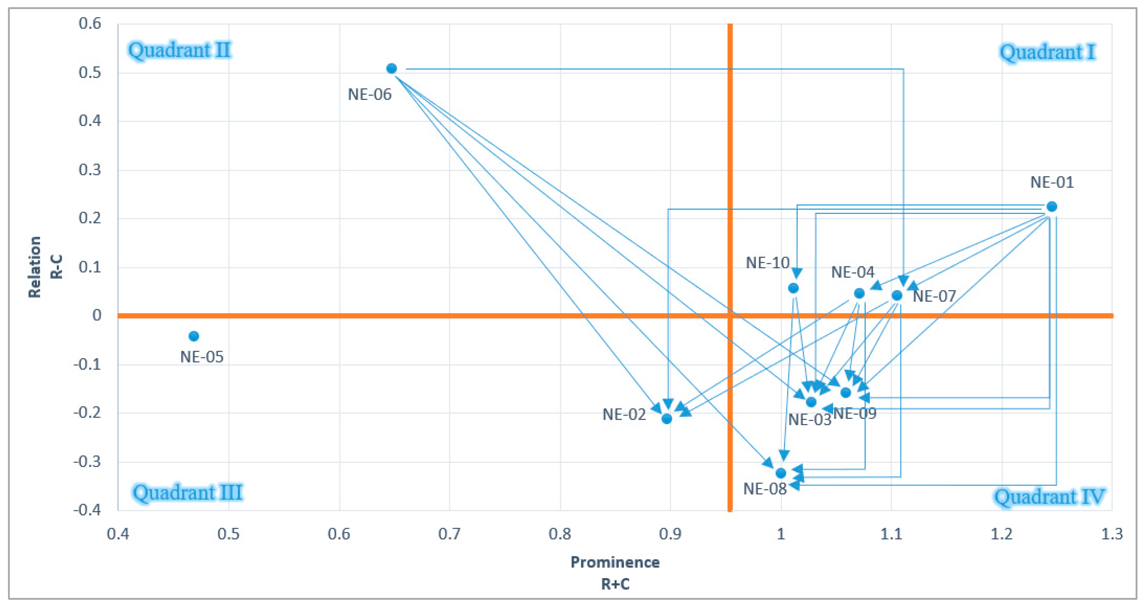
4.1. Negative Effect Identification and Prioritization by Fuzzy DEMATEL Method

The analysis and assessment of the pandemic’s negative effects on logistics activities play a decisive role in determining the appropriate recovery strategy. Based on previous studies and expert surveys, there are ten negative impacts identified concerning logistics activities in Vietnam, as presented in

Table 4. List of pandemic negative effects on logistics activities in Vietnam.

Notation	Category	Negative Effect	Reference
NE-01	Operation	Incurred costs	[63]
NE-02	Operation	The decline in warehouse capacity	[64,65]
NE-03	Operation	Goods volume reduction	[66]
NE-04	Operation	Shortage of workforce	[63,67,68]
NE-05	Operation	Damaged product increasing	[69]
NE-06	Networking	Disruption of the logistics network	[63,70]
NE-07	Networking	Shortage of 3PL services	[65]
NE-08	Networking	Trading restrictions	[68]
NE-09	Transportation	Uncertain delivery time	[64]
NE-10	Transportation	Restrictions on modes of transport	[70]

. The negative impacts on operations are as follows:

• The increase in costs in all logistics activities (NE-01);
• Decline in inventory capacity due to limited warehouse operations (NE-02);
• Declining demand and supply constraints lead to a decrease in the volume of goods throughout the supply chain (NE-03);
• The social health situation, as well as movement restrictions to control the epidemic, have severely reduced the workforce in the logistics sector (NE-04);
• Disruption of transportation operations resulting in increased goods damage (NE-05).

In addition, the pandemic also has negative effects on logistics activities in terms of networking between players and transportation in the supply chain as follows:

• The disruption of the global logistics network is the cause of the local breakdown (NE-06);
• Many third-party logistics service providers have to close temporarily or permanently resulting in shortages of services (NE-07);
• Trading activities face many obstacles due to the blockade of border gates, ports, and economic zones (NE-08).
• Transportation activities have been greatly hindered due to epidemic control. Among them, delay in delivery time (NE-09) and limited choice of transportation modes (NE-10) are two noticeable negative effects.

To analyze the influence of negative effects on the logistics activities of Vietnam, ten experts were surveyed. These experts have nine to fifteen years of experience in logistics and public policy management in Vietnam. In this case study, we assume that the experts have an equal weight coefficient. First, experts provide linguistic evaluations about the influence of negative effects as pairwise comparisons. Table 5 below describes the linguistic evaluation of influence by Expert 1. This process was repeated for all experts who participated in the study. The individualistic direct influence evaluation matrices are constructed by converting linguistic evaluation intro SFNs according to the relationships in Table 2. Then, the aggregated direct influence matrix is constructed using SWAM according to Equation (7), as shown in Table 6.

Table 5. The linguistics evaluation of NEs’ influence by Expert 1 $(Q^1={\left[q_{jl}^1\right]}_{JxJ}$).

Negative Effect	NE-01	NE-02	NE-03	NE-04	NE-05	NE-06	NE-07	NE-08	NE-09	NE-10
NE-01	NI	MI	SI	MI	SI	WI	MI	MI	SI	SI
NE-02	WI	NI	MI	MI	NI	WI	NI	NI	MI	SI
NE-03	SI	SI	NI	MI	NI	NI	WI	NI	SI	MI
NE-04	SI	MI	SI	NI	WI	NI	WI	NI	NI	WI
NE-05	NI	WI	WI	WI	NI	WI	NI	WI	NI	NI
NE-06	WI	NI	MI	MI	WI	NI	SI	MI	MI	MI
NE-07	NI	MI	WI	NI	NI	MI	NI	NI	NI	MI
NE-08	WI	NI	MI	SI	WI	NI	MI	NI	WI	MI
NE-09	SI	SI	WI	NI	WI	WI	SI	SI	NI	SI
NE-10	MI	WI	MI	MI	NI	NI	NI	MI	NI	NI

Table 5. The linguistics evaluation of NEs’ influence by Expert 1 $(Q^1={\left[q_{jl}^1\right]}_{JxJ}$).

Negative Effect	NE-01	NE-02	NE-03	NE-04	NE-05	NE-06	NE-07	NE-08	NE-09	NE-10
NE-01	NI	MI	SI	MI	SI	WI	MI	MI	SI	SI
NE-02	WI	NI	MI	MI	NI	WI	NI	NI	MI	SI
NE-03	SI	SI	NI	MI	NI	NI	WI	NI	SI	MI
NE-04	SI	MI	SI	NI	WI	NI	WI	NI	NI	WI
NE-05	NI	WI	WI	WI	NI	WI	NI	WI	NI	NI
NE-06	WI	NI	MI	MI	WI	NI	SI	MI	MI	MI
NE-07	NI	MI	WI	NI	NI	MI	NI	NI	NI	MI
NE-08	WI	NI	MI	SI	WI	NI	MI	NI	WI	MI
NE-09	SI	SI	WI	NI	WI	WI	SI	SI	NI	SI
NE-10	MI	WI	MI	MI	NI	NI	NI	MI	NI	NI

Table 6. The aggregated direct influence matrix $\left(D^{*}\right)$.

Negative Effect	NE-01	NE-02	NE-03	NE-04	NE-05
NE-01	(0.00, 0.30, 0.20)	(0.74, 0.18, 0.48)	(0.69, 0.19, 0.46)	(0.71, 0.19, 0.48)	(0.42, 0.26, 0.37)
NE-02	(0.56, 0.22, 0.44)	(0.00, 0.30, 0.20)	(0.54, 0.23, 0.39)	(0.45, 0.24, 0.30)	(0.41, 0.26, 0.38)
NE-03	(0.67, 0.20, 0.47)	(0.57, 0.23, 0.44)	(0.00, 0.30, 0.20)	(0.52, 0.23, 0.39)	(0.44, 0.25, 0.38)
NE-04	(0.61, 0.21, 0.44)	(0.68, 0.20, 0.46)	(0.64, 0.20, 0.44)	(0.00, 0.30, 0.20)	(0.57, 0.22, 0.44)
NE-05	(0.61, 0.21, 0.44)	(0.51, 0.23, 0.39)	(0.48, 0.23, 0.31)	(0.39, 0.25, 0.28)	(0.00, 0.30, 0.20)
NE-06	(0.65, 0.21, 0.47)	(0.60, 0.21, 0.40)	(0.59, 0.21, 0.40)	(0.59, 0.22, 0.44)	(0.46, 0.25, 0.38)
NE-07	(0.63, 0.22, 0.47)	(0.71, 0.19, 0.48)	(0.67, 0.20, 0.47)	(0.57, 0.24, 0.48)	(0.44, 0.24, 0.30)
NE-08	(0.42, 0.26, 0.37)	(0.45, 0.24, 0.30)	(0.50, 0.22, 0.32)	(0.67, 0.20, 0.47)	(0.49, 0.23, 0.38)
NE-09	(0.54, 0.24, 0.44)	(0.53, 0.23, 0.44)	(0.70, 0.19, 0.48)	(0.53, 0.23, 0.39)	(0.39, 0.25, 0.28)
NE-10	(0.52, 0.23, 0.39)	(0.50, 0.24, 0.38)	(0.65, 0.20, 0.47)	(0.68, 0.21, 0.49)	(0.54, 0.24, 0.44)
Negative Effect	NE-06	NE-07	NE-08	NE-09	NE-10
NE-01	(0.58, 0.21, 0.40)	(0.66, 0.20, 0.47)	(0.78, 0.17, 0.47)	(0.75, 0.18, 0.48)	(0.69, 0.19, 0.46)
NE-02	(0.32, 0.26, 0.25)	(0.57, 0.23, 0.44)	(0.57, 0.22, 0.44)	(0.51, 0.22, 0.32)	(0.54, 0.24, 0.44)
NE-03	(0.36, 0.26, 0.27)	(0.50, 0.24, 0.39)	(0.64, 0.21, 0.47)	(0.59, 0.22, 0.44)	(0.50, 0.24, 0.39)
NE-04	(0.34, 0.26, 0.26)	(0.53, 0.23, 0.39)	(0.61, 0.21, 0.44)	(0.64, 0.20, 0.44)	(0.68, 0.21, 0.49)
NE-05	(0.25, 0.27, 0.23)	(0.41, 0.26, 0.37)	(0.43, 0.24, 0.29)	(0.54, 0.23, 0.39)	(0.35, 0.26, 0.27)
NE-06	(0.00, 0.30, 0.20)	(0.68, 0.20, 0.46)	(0.69, 0.19, 0.46)	(0.57, 0.22, 0.40)	(0.49, 0.24, 0.38)
NE-07	(0.38, 0.25, 0.27)	(0.00, 0.30, 0.20)	(0.66, 0.21, 0.47)	(0.67, 0.2, 0.47)	(0.61, 0.21, 0.44)
NE-08	(0.23, 0.28, 0.22)	(0.62, 0.21, 0.44)	(0.00, 0.30, 0.20)	(0.61, 0.21, 0.44)	(0.52, 0.25, 0.44)
NE-09	(0.32, 0.26, 0.25)	(0.66, 0.20, 0.47)	(0.62, 0.22, 0.47)	(0.00, 0.30, 0.20)	(0.58, 0.23, 0.44)
NE-10	(0.41, 0.25, 0.29)	(0.59, 0.22, 0.44)	(0.71, 0.19, 0.48)	(0.60, 0.23, 0.48)	(0.00, 0.30, 0.20)

For normalization, the aggregated direct influence matrix ($D^{*})$ is split into three sub-matrices. These submatrices are normalized according to Equations (24)–(26). The initial direct influence submatrices are shown in

Table A1. The initial direct influence submatrix for the membership parameters $\left(Y^{\alpha }\right)$.

Negative Effect	NE-01	NE-02	NE-03	NE-04	NE-05	NE-06	NE-07	NE-08	NE-09	NE-10
NE-01	0.00	0.12	0.11	0.12	0.07	0.10	0.11	0.13	0.12	0.11
NE-02	0.09	0.00	0.09	0.08	0.07	0.05	0.09	0.10	0.09	0.09
NE-03	0.11	0.09	0.00	0.09	0.07	0.06	0.08	0.11	0.10	0.08
NE-04	0.10	0.11	0.11	0.00	0.10	0.06	0.09	0.10	0.11	0.11
NE-05	0.10	0.08	0.08	0.07	0.00	0.04	0.07	0.07	0.09	0.06
NE-06	0.11	0.10	0.10	0.10	0.08	0.00	0.11	0.11	0.09	0.08
NE-07	0.10	0.12	0.11	0.10	0.07	0.06	0.00	0.11	0.11	0.10
NE-08	0.07	0.08	0.08	0.11	0.08	0.04	0.10	0.00	0.10	0.09
NE-09	0.09	0.09	0.12	0.09	0.07	0.05	0.11	0.10	0.00	0.10
NE-10	0.09	0.08	0.11	0.11	0.09	0.07	0.10	0.12	0.10	0.00

,

Table A2. The initial direct influence submatrix for the non-membership parameters $\left(Y^{\beta }\right)$.

Negative Effect	NE-01	NE-02	NE-03	NE-04	NE-05	NE-06	NE-07	NE-08	NE-09	NE-10
NE-01	0.12	0.07	0.07	0.07	0.10	0.08	0.08	0.06	0.07	0.07
NE-02	0.09	0.12	0.09	0.09	0.10	0.10	0.09	0.09	0.09	0.09
NE-03	0.08	0.09	0.12	0.09	0.10	0.10	0.09	0.08	0.08	0.09
NE-04	0.08	0.07	0.08	0.12	0.09	0.10	0.09	0.08	0.08	0.08
NE-05	0.08	0.09	0.09	0.10	0.12	0.11	0.10	0.09	0.09	0.10
NE-06	0.08	0.08	0.08	0.08	0.10	0.12	0.07	0.07	0.08	0.09
NE-07	0.08	0.07	0.08	0.09	0.09	0.10	0.12	0.08	0.08	0.08
NE-08	0.10	0.09	0.09	0.08	0.09	0.11	0.08	0.12	0.08	0.09
NE-09	0.09	0.09	0.07	0.09	0.10	0.10	0.08	0.08	0.12	0.09
NE-10	0.09	0.09	0.08	0.08	0.09	0.09	0.09	0.07	0.09	0.12

and

Table A3. The initial direct influence submatrix for the hesitancy parameters $\left(Y^{\gamma }\right)$.

Negative Effect	NE-01	NE-02	NE-03	NE-04	NE-05	NE-06	NE-07	NE-08	NE-09	NE-10
NE-01	0.04	0.10	0.10	0.10	0.08	0.08	0.10	0.10	0.10	0.10
NE-02	0.09	0.04	0.08	0.06	0.08	0.05	0.09	0.09	0.07	0.09
NE-03	0.10	0.09	0.04	0.08	0.08	0.06	0.08	0.10	0.09	0.08
NE-04	0.09	0.10	0.09	0.04	0.09	0.06	0.08	0.09	0.09	0.10
NE-05	0.09	0.08	0.07	0.06	0.04	0.05	0.08	0.06	0.08	0.06
NE-06	0.10	0.09	0.09	0.09	0.08	0.04	0.10	0.10	0.08	0.08
NE-07	0.10	0.10	0.10	0.10	0.06	0.06	0.04	0.10	0.10	0.09
NE-08	0.08	0.06	0.07	0.10	0.08	0.05	0.09	0.04	0.09	0.10
NE-09	0.09	0.09	0.10	0.08	0.06	0.05	0.10	0.10	0.04	0.10
NE-10	0.08	0.08	0.10	0.10	0.09	0.06	0.10	0.10	0.10	0.04

. According to Equations (27)–(29), the total influence submatrices $\left(X^{\alpha },X^{\beta }, \mathrm{and} X^{\gamma }\right)$ are determined. As shown in Table 7, the total influence matrix $\left(X^{*}\right)$ is constructed by combining submatrices.

Table 6. The aggregated direct influence matrix $\left(D^{*}\right)$.

Negative Effect	NE-01	NE-02	NE-03	NE-04	NE-05
NE-01	(0.00, 0.30, 0.20)	(0.74, 0.18, 0.48)	(0.69, 0.19, 0.46)	(0.71, 0.19, 0.48)	(0.42, 0.26, 0.37)
NE-02	(0.56, 0.22, 0.44)	(0.00, 0.30, 0.20)	(0.54, 0.23, 0.39)	(0.45, 0.24, 0.30)	(0.41, 0.26, 0.38)
NE-03	(0.67, 0.20, 0.47)	(0.57, 0.23, 0.44)	(0.00, 0.30, 0.20)	(0.52, 0.23, 0.39)	(0.44, 0.25, 0.38)
NE-04	(0.61, 0.21, 0.44)	(0.68, 0.20, 0.46)	(0.64, 0.20, 0.44)	(0.00, 0.30, 0.20)	(0.57, 0.22, 0.44)
NE-05	(0.61, 0.21, 0.44)	(0.51, 0.23, 0.39)	(0.48, 0.23, 0.31)	(0.39, 0.25, 0.28)	(0.00, 0.30, 0.20)
NE-06	(0.65, 0.21, 0.47)	(0.60, 0.21, 0.40)	(0.59, 0.21, 0.40)	(0.59, 0.22, 0.44)	(0.46, 0.25, 0.38)
NE-07	(0.63, 0.22, 0.47)	(0.71, 0.19, 0.48)	(0.67, 0.20, 0.47)	(0.57, 0.24, 0.48)	(0.44, 0.24, 0.30)
NE-08	(0.42, 0.26, 0.37)	(0.45, 0.24, 0.30)	(0.50, 0.22, 0.32)	(0.67, 0.20, 0.47)	(0.49, 0.23, 0.38)
NE-09	(0.54, 0.24, 0.44)	(0.53, 0.23, 0.44)	(0.70, 0.19, 0.48)	(0.53, 0.23, 0.39)	(0.39, 0.25, 0.28)
NE-10	(0.52, 0.23, 0.39)	(0.50, 0.24, 0.38)	(0.65, 0.20, 0.47)	(0.68, 0.21, 0.49)	(0.54, 0.24, 0.44)
Negative Effect	NE-06	NE-07	NE-08	NE-09	NE-10
NE-01	(0.58, 0.21, 0.40)	(0.66, 0.20, 0.47)	(0.78, 0.17, 0.47)	(0.75, 0.18, 0.48)	(0.69, 0.19, 0.46)
NE-02	(0.32, 0.26, 0.25)	(0.57, 0.23, 0.44)	(0.57, 0.22, 0.44)	(0.51, 0.22, 0.32)	(0.54, 0.24, 0.44)
NE-03	(0.36, 0.26, 0.27)	(0.50, 0.24, 0.39)	(0.64, 0.21, 0.47)	(0.59, 0.22, 0.44)	(0.50, 0.24, 0.39)
NE-04	(0.34, 0.26, 0.26)	(0.53, 0.23, 0.39)	(0.61, 0.21, 0.44)	(0.64, 0.20, 0.44)	(0.68, 0.21, 0.49)
NE-05	(0.25, 0.27, 0.23)	(0.41, 0.26, 0.37)	(0.43, 0.24, 0.29)	(0.54, 0.23, 0.39)	(0.35, 0.26, 0.27)
NE-06	(0.00, 0.30, 0.20)	(0.68, 0.20, 0.46)	(0.69, 0.19, 0.46)	(0.57, 0.22, 0.40)	(0.49, 0.24, 0.38)
NE-07	(0.38, 0.25, 0.27)	(0.00, 0.30, 0.20)	(0.66, 0.21, 0.47)	(0.67, 0.2, 0.47)	(0.61, 0.21, 0.44)
NE-08	(0.23, 0.28, 0.22)	(0.62, 0.21, 0.44)	(0.00, 0.30, 0.20)	(0.61, 0.21, 0.44)	(0.52, 0.25, 0.44)
NE-09	(0.32, 0.26, 0.25)	(0.66, 0.20, 0.47)	(0.62, 0.22, 0.47)	(0.00, 0.30, 0.20)	(0.58, 0.23, 0.44)
NE-10	(0.41, 0.25, 0.29)	(0.59, 0.22, 0.44)	(0.71, 0.19, 0.48)	(0.60, 0.23, 0.48)	(0.00, 0.30, 0.20)

For normalization, the aggregated direct influence matrix ($D^{*})$ is split into three sub-matrices. These submatrices are normalized according to Equations (24)–(26). The initial direct influence submatrices are shown in Table A1, Table A2 and Table A3. According to Equations (27)–(29), the total influence submatrices $\left(X^{\alpha },X^{\beta }, \mathrm{and} X^{\gamma }\right)$ are determined. As shown in Table 7, the total influence matrix $\left(X^{*}\right)$ is constructed by combining submatrices.

Table 7. The total influence matrix $\left(X^{*}\right)$.

Negative Effect	NE-01	NE-02	NE-03	NE-04	NE-05
NE-01	(0.50, 0.73, 0.50)	(0.62, 0.67, 0.54)	(0.63, 0.66, 0.54)	(0.60, 0.69, 0.54)	(0.47, 0.78, 0.47)
NE-02	(0.46, 0.82, 0.48)	(0.39, 0.83, 0.42)	(0.48, 0.78, 0.46)	(0.45, 0.82, 0.44)	(0.37, 0.90, 0.42)
NE-03	(0.50, 0.79, 0.51)	(0.50, 0.79, 0.49)	(0.43, 0.79, 0.44)	(0.48, 0.81, 0.48)	(0.40, 0.88, 0.44)
NE-04	(0.53, 0.75, 0.52)	(0.55, 0.73, 0.51)	(0.56, 0.71, 0.50)	(0.44, 0.79, 0.45)	(0.45, 0.82, 0.46)
NE-05	(0.43, 0.83, 0.43)	(0.42, 0.82, 0.41)	(0.43, 0.80, 0.40)	(0.40, 0.85, 0.39)	(0.28, 0.94, 0.34)
NE-06	(0.54, 0.75, 0.53)	(0.54, 0.74, 0.50)	(0.56, 0.72, 0.50)	(0.53, 0.76, 0.50)	(0.44, 0.83, 0.45)
NE-07	(0.54, 0.76, 0.53)	(0.56, 0.74, 0.52)	(0.57, 0.72, 0.52)	(0.53, 0.77, 0.52)	(0.43, 0.84, 0.44)
NE-08	(0.44, 0.82, 0.47)	(0.46, 0.80, 0.44)	(0.48, 0.77, 0.44)	(0.48, 0.80, 0.47)	(0.39, 0.88, 0.41)
NE-09	(0.49, 0.80, 0.51)	(0.50, 0.78, 0.50)	(0.54, 0.74, 0.50)	(0.49, 0.80, 0.48)	(0.40, 0.87, 0.42)
NE-10	(0.51, 0.78, 0.52)	(0.52, 0.77, 0.50)	(0.55, 0.73, 0.51)	(0.53, 0.77, 0.52)	(0.44, 0.85, 0.47)
Negative Effect	NE-06	NE-07	NE-08	NE-09	NE-10
NE-01	(0.40, 0.79, 0.38)	(0.60, 0.69, 0.55)	(0.66, 0.65, 0.57)	(0.64, 0.66, 0.55)	(0.59, 0.71, 0.54)
NE-02	(0.29, 0.93, 0.31)	(0.47, 0.82, 0.48)	(0.50, 0.78, 0.49)	(0.48, 0.79, 0.45)	(0.45, 0.85, 0.47)
NE-03	(0.31, 0.91, 0.33)	(0.48, 0.81, 0.49)	(0.54, 0.76, 0.52)	(0.52, 0.77, 0.50)	(0.47, 0.83, 0.48)
NE-04	(0.34, 0.86, 0.33)	(0.52, 0.76, 0.51)	(0.57, 0.71, 0.53)	(0.56, 0.72, 0.52)	(0.53, 0.77, 0.52)
NE-05	(0.26, 0.96, 0.27)	(0.40, 0.85, 0.42)	(0.44, 0.80, 0.41)	(0.44, 0.81, 0.42)	(0.38, 0.88, 0.39)
NE-06	(0.28, 0.88, 0.32)	(0.55, 0.75, 0.52)	(0.59, 0.71, 0.54)	(0.56, 0.73, 0.51)	(0.51, 0.79, 0.50)
NE-07	(0.34, 0.87, 0.34)	(0.45, 0.79, 0.47)	(0.58, 0.72, 0.54)	(0.57, 0.73, 0.53)	(0.52, 0.78, 0.52)
NE-08	(0.28, 0.93, 0.30)	(0.48, 0.80, 0.47)	(0.42, 0.80, 0.44)	(0.49, 0.77, 0.48)	(0.45, 0.84, 0.47)
NE-09	(0.31, 0.91, 0.33)	(0.51, 0.78, 0.51)	(0.54, 0.75, 0.53)	(0.43, 0.79, 0.46)	(0.48, 0.82, 0.50)
NE-10	(0.34, 0.88, 0.34)	(0.53, 0.77, 0.52)	(0.58, 0.72, 0.54)	(0.55, 0.75, 0.53)	(0.42, 0.83, 0.46)

Table 7. The total influence matrix $\left(X^{*}\right)$.

Negative Effect	NE-01	NE-02	NE-03	NE-04	NE-05
NE-01	(0.50, 0.73, 0.50)	(0.62, 0.67, 0.54)	(0.63, 0.66, 0.54)	(0.60, 0.69, 0.54)	(0.47, 0.78, 0.47)
NE-02	(0.46, 0.82, 0.48)	(0.39, 0.83, 0.42)	(0.48, 0.78, 0.46)	(0.45, 0.82, 0.44)	(0.37, 0.90, 0.42)
NE-03	(0.50, 0.79, 0.51)	(0.50, 0.79, 0.49)	(0.43, 0.79, 0.44)	(0.48, 0.81, 0.48)	(0.40, 0.88, 0.44)
NE-04	(0.53, 0.75, 0.52)	(0.55, 0.73, 0.51)	(0.56, 0.71, 0.50)	(0.44, 0.79, 0.45)	(0.45, 0.82, 0.46)
NE-05	(0.43, 0.83, 0.43)	(0.42, 0.82, 0.41)	(0.43, 0.80, 0.40)	(0.40, 0.85, 0.39)	(0.28, 0.94, 0.34)
NE-06	(0.54, 0.75, 0.53)	(0.54, 0.74, 0.50)	(0.56, 0.72, 0.50)	(0.53, 0.76, 0.50)	(0.44, 0.83, 0.45)
NE-07	(0.54, 0.76, 0.53)	(0.56, 0.74, 0.52)	(0.57, 0.72, 0.52)	(0.53, 0.77, 0.52)	(0.43, 0.84, 0.44)
NE-08	(0.44, 0.82, 0.47)	(0.46, 0.80, 0.44)	(0.48, 0.77, 0.44)	(0.48, 0.80, 0.47)	(0.39, 0.88, 0.41)
NE-09	(0.49, 0.80, 0.51)	(0.50, 0.78, 0.50)	(0.54, 0.74, 0.50)	(0.49, 0.80, 0.48)	(0.40, 0.87, 0.42)
NE-10	(0.51, 0.78, 0.52)	(0.52, 0.77, 0.50)	(0.55, 0.73, 0.51)	(0.53, 0.77, 0.52)	(0.44, 0.85, 0.47)
Negative Effect	NE-06	NE-07	NE-08	NE-09	NE-10
NE-01	(0.40, 0.79, 0.38)	(0.60, 0.69, 0.55)	(0.66, 0.65, 0.57)	(0.64, 0.66, 0.55)	(0.59, 0.71, 0.54)
NE-02	(0.29, 0.93, 0.31)	(0.47, 0.82, 0.48)	(0.50, 0.78, 0.49)	(0.48, 0.79, 0.45)	(0.45, 0.85, 0.47)
NE-03	(0.31, 0.91, 0.33)	(0.48, 0.81, 0.49)	(0.54, 0.76, 0.52)	(0.52, 0.77, 0.50)	(0.47, 0.83, 0.48)
NE-04	(0.34, 0.86, 0.33)	(0.52, 0.76, 0.51)	(0.57, 0.71, 0.53)	(0.56, 0.72, 0.52)	(0.53, 0.77, 0.52)
NE-05	(0.26, 0.96, 0.27)	(0.40, 0.85, 0.42)	(0.44, 0.80, 0.41)	(0.44, 0.81, 0.42)	(0.38, 0.88, 0.39)
NE-06	(0.28, 0.88, 0.32)	(0.55, 0.75, 0.52)	(0.59, 0.71, 0.54)	(0.56, 0.73, 0.51)	(0.51, 0.79, 0.50)
NE-07	(0.34, 0.87, 0.34)	(0.45, 0.79, 0.47)	(0.58, 0.72, 0.54)	(0.57, 0.73, 0.53)	(0.52, 0.78, 0.52)
NE-08	(0.28, 0.93, 0.30)	(0.48, 0.80, 0.47)	(0.42, 0.80, 0.44)	(0.49, 0.77, 0.48)	(0.45, 0.84, 0.47)
NE-09	(0.31, 0.91, 0.33)	(0.51, 0.78, 0.51)	(0.54, 0.75, 0.53)	(0.43, 0.79, 0.46)	(0.48, 0.82, 0.50)
NE-10	(0.34, 0.88, 0.34)	(0.53, 0.77, 0.52)	(0.58, 0.72, 0.54)	(0.55, 0.75, 0.53)	(0.42, 0.83, 0.46)

According to Equations (31) and (32), the SF row sum $\left({\tilde{r}}_j\right)$ and SF column sum $\left({\tilde{c}}_j\right)$ of the total influence matrix are computed. Next, the defuzzification process is performed for row and column sums according to Equation (13). Finally, the prominence, the relation, and the absolute weight of the NEs are determined according to Equation (33). The results of the SF DEMATEL method are shown in

Table 8. The spherical fuzzy DEMATEL results.

Negative Effect	${\tilde{\mathit{r}}}_{\mathit{j}}$	${\mathit{r}}_{\mathit{j}}$	${\tilde{\mathit{c}}}_{\mathit{j}}$	${\mathit{c}}_{\mathit{j}}$	Prominence ${\mathit{r}}_{\mathit{j}}+{\mathit{c}}_{\mathit{j}}$	Relation ${\mathit{r}}_{\mathit{j}}-{\mathit{c}}_{\mathit{j}}$	Weight
NE-01	(0.992, 0.029, 0.129)	0.735	(0.970, 0.086, 0.239)	0.511	1.246	0.224	0.131
NE-02	(0.941, 0.155, 0.330)	0.342	(0.976, 0.069, 0.217)	0.555	0.897	−0.212	0.094
NE-03	(0.957, 0.126, 0.285)	0.425	(0.981, 0.050, 0.192)	0.603	1.028	−0.178	0.108
NE-04	(0.976, 0.066, 0.215)	0.558	(0.970, 0.089, 0.239)	0.513	1.071	0.045	0.112
NE-05	(0.903, 0.199, 0.400)	0.213	(0.917, 0.214, 0.384)	0.256	0.469	−0.043	0.049
NE-06	(0.978, 0.067, 0.205)	0.578	(0.812, 0.318, 0.495)	0.069	0.648	0.509	0.068
NE-07	(0.978, 0.073, 0.208)	0.574	(0.973, 0.083, 0.229)	0.532	1.105	0.042	0.116
NE-08	(0.941, 0.135, 0.328)	0.338	(0.986, 0.048, 0.164)	0.662	1.003	−0.324	0.105
NE-09	(0.961, 0.111, 0.271)	0.451	(0.982, 0.057, 0.190)	0.608	1.059	−0.158	0.111
NE-10	(0.973, 0.089, 0.229)	0.534	(0.965, 0.119, 0.260)	0.478	1.012	0.056	0.106

. As discussed in Section 3.2, negative effects, which have positive relation values $\left(r_j-c_j\right)$, are grouped into cause factors. The negative effects that belong to the group of cause factors include the incurred costs (NE-01), shortage of workforce (NE-04), disruption of the logistics network (NE-06), Shortage of 3PL services (NE-07), and restrictions on modes of transport (NE-10). In particular, the incurred costs (NE-01) and the logistics network disruption (NE-06) are the negative effects that have the greatest influence on the rest. In contrast, the decline in warehouse capacity (NE-02), goods volume reduction (NE-03), damaged product increase (NE-05), trading restrictions (NE-08), and uncertain delivery time (NE-09) belongs to the group of effect factors that are influenced by the group of cause factors.

As discussed in Step 9 of the SF DEMATEL method, the four-quadrant network relation map of negative effects is presented in Figure 4. In the upper right quadrant are intertwined givers with both high prominence and relation values. Next, the NE in the upper left quadrant is the group of autonomous givers. This category has a low prominence but high relation. The third category is named the autonomous receivers, which have both low prominence and low relation, in the lower right quadrant. Finally, there are the intertwined receivers in the lower left quadrant with high prominence and low connection to the remaining NEs.

Table 9. Negative effect classification.

Category	Negative Effects
Intertwined givers	NE-01, NE-04, NE-07, and NE-10
Autonomous givers	NE-06
Intertwined receivers	NE-03, NE-08, and NE-09
Autonomous receivers	NE-02 and NE-05

summarizes the categories according to the results of this classification.

Based on the classifications shown in Table 9, the development of strategies to mitigate the negative effects of logistics activities should give more consideration to intertwined givers and autonomous givers. Figure 4 illustrates that most negative effects are affected by NE-01 and NE-06. Therefore, operational strategies that are highly effective for mitigating these two negative effects are believed to provide significant overall improvements. It was then recommended that logistics managers in Vietnam focus on operational strategies that address the cause-factor negative effects, such as NE-04, NE-07, and NE-10.

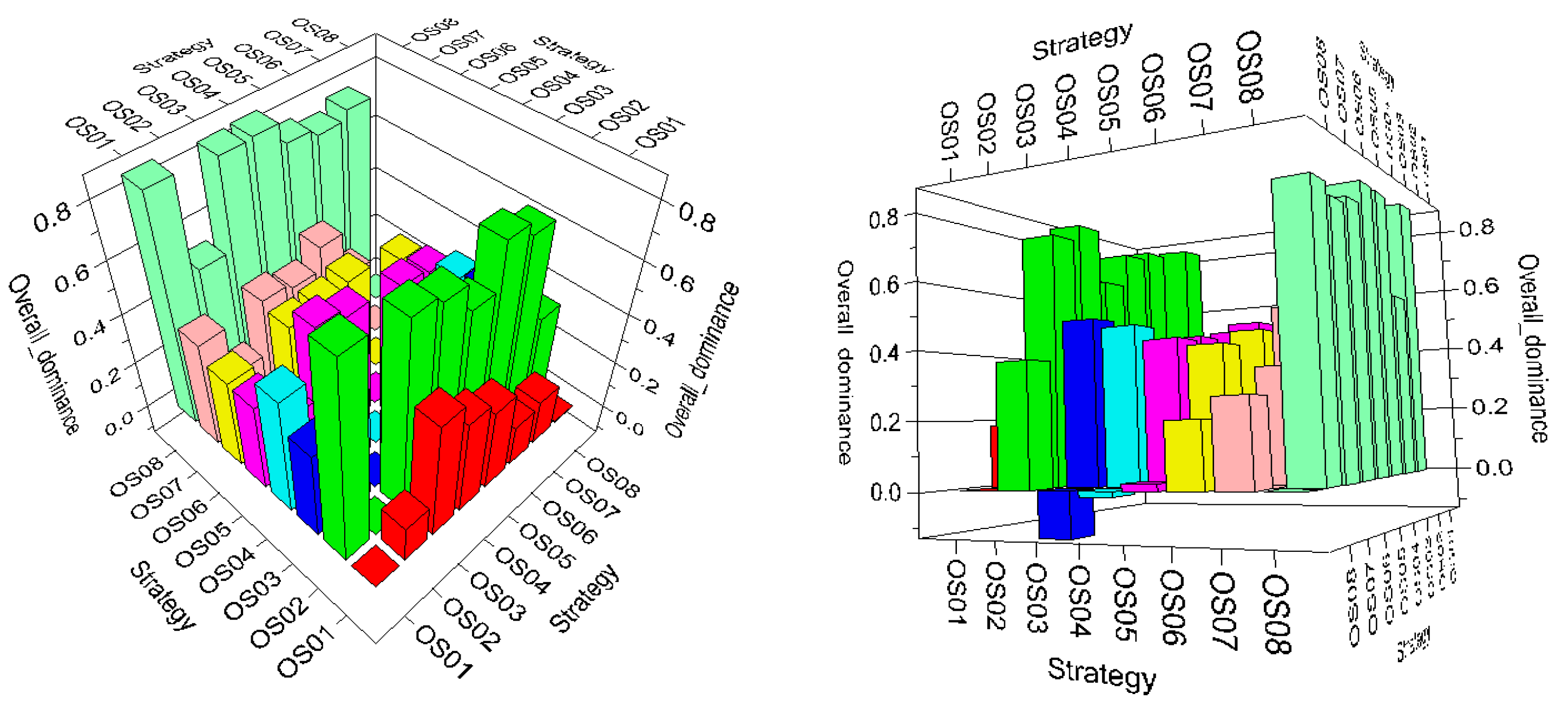
4.2. The Operational Strategies Evaluation by the SF TODIM’MC Method

After performing the analysis in Stage 1, the absolute weights of the negative effects are determined. At this stage, this study conducts an assessment of the mitigation ability’s strategies, which are suggested by previous strategy development studies and logistics experts in Vietnam. As shown in

Table 10. Post-COVID-19 operational strategies for logistics activities.

Notation	Operational Strategy	Reference
OS-01	Core competencies focusing	[64]
OS-02	Omni-channel distribution model	[64,71]
OS-03	Develop local 3PL providers	[64]
OS-04	Utilize temporary labor but prioritize dedicated labor	[72]
OS-05	Backup route	[70]
OS-06	Utilize of outsourced vehicles with high transparency	[64,73]
OS-07	Smart systems and autonomous vehicles	[39,74]
OS-08	Reserve capacity	[64,71]

, the suggested operational strategies include:

• Core competencies focusing: Under normal circumstances, companies tend to take on most of the logistics that they can afford and be more cost effective. However, in post-pandemic conditions, companies should focus on their core competencies and leverage outsourced resources. The advantage of this strategy is to optimize internal resources and transfer ownership risk to third parties.
• Omni-channel distribution model: To increase the flexibility of the distribution network, omni-channel distribution models should be considered by logistics managers. Customers or manufacturers at the bottom of the supply chain will have more choices with a distribution network that combines brick-and-mortar stores, smart pick-ups points, and online shopping.
• Develop local 3PL providers: The interregional 3PLs are considered to be more comprehensive and effective in both cost and performance. However, developing local 3PLs is a safe solution for companies’ logistics problems to reduce dependence when unexpected events occur.
• Utilize temporary labor but prioritize dedicated labor: To face the challenge of labor shortages, logistics companies are suggested to develop a temporary skilled workforce that rotates between companies. However, managers are also more interested in the dedicated workforce. Special preferential policies for dedicated employees are the motivation for them to maintain service in the most difficult situations. For sustainable development, companies are suggested to strike a balance between these two workforce groups.
• Backup route: Disruption in transportation operations is a cause of direct or indirect costs incurred by companies during and after the pandemic. The backup route strategy requires larger investments but reduces response time when disruptions occur.
• Utilize outsourced vehicles with high transparency: Because of geographical restrictions during and after the pandemic, logistics companies’ transportation activities are restricted to specific regions. The consequence is an imbalance in regional transport capacity. Therefore, a strategy utilizing outsourcing according to the principles of the sharing economy is suggested. However, transparency needs to be noticed and optimized by tracking and information-sharing technologies.
• Smart systems and autonomous vehicles: The larger companies may consider unmanned transport vehicles for transportation between fixed locations. For warehouse operations, smart systems can be invested to increase accuracy and efficiency. Although this strategy requires a large investment, it promises long-term benefits because of its independence from the human factor in operations.
• Reserve capacity: The reserve capacity can be calculated by managers to increase company readiness. This strategy may result in additional costs to keep resources idle, but it helps the company reduce the risk of disruption.

In the next step, the potential performance of the OSs is evaluated linguistically according to the NEs by each expert. The survey results of Expert 1 are presented in

Table A4. The linguistic judgment of operational strategy by Expert 1 $\left(g_{ij}^1\right)$.

Strategy	NE-01	NE-02	NE-03	NE-04	NE-05	NE-06	NE-07	NE-08	NE-09	NE-10
OS-01	AH	SH	SL	M	M	L	AH	SL	VH	SL
OS-02	AL	VH	SH	VH	L	H	L	SL	AH	VL
OS-03	AH	AH	L	AH	L	AL	AH	M	H	SH
OS-04	VL	H	SH	H	VH	VH	AH	M	L	H
OS-05	AH	AH	H	AL	M	H	L	VLI	H	H
OS-06	M	H	VH	SH	AH	VH	M	M	M	VH
OS-07	VL	SL	SL	H	AH	SH	SH	M	M	VL
OS-08	AH	L	L	AH	H	VH	SL	ALI	SL	AH

. The linguistic terms are converted into SFNs according to Table 3. As a result, the SF decision matrix of Expert 1 is defined as shown in

Table A5. The spherical fuzzy decision matrix by Expert 1 $\left({\tilde{M}}_{ij}^1\right)$.

Strategy	NE-01	NE-02	NE-03	NE-04	NE-05
OS-01	(0.9, 0.1, 0.1)	(0.6, 0.4, 0.4)	(0.4, 0.6, 0.4)	(0.5, 0.5, 0.5)	(0.5, 0.5, 0.5)
OS-02	(0.1, 0.9, 0.1)	(0.8, 0.2, 0.2)	(0.6, 0.4, 0.4)	(0.8, 0.2, 0.2)	(0.3, 0.7, 0.3)
OS-03	(0.9, 0.1, 0.1)	(0.9, 0.1, 0.1)	(0.3, 0.7, 0.3)	(0.9, 0.1, 0.1)	(0.3, 0.7, 0.3)
OS-04	(0.2, 0.8, 0.2)	(0.7, 0.3, 0.3)	(0.6, 0.4, 0.4)	(0.7, 0.3, 0.3)	(0.8, 0.2, 0.2)
OS-05	(0.9, 0.1, 0.1)	(0.9, 0.1, 0.1)	(0.7, 0.3, 0.3)	(0.1, 0.9, 0.1)	(0.5, 0.5, 0.5)
OS-06	(0.5, 0.5, 0.5)	(0.7, 0.3, 0.3)	(0.8, 0.2, 0.2)	(0.6, 0.4, 0.4)	(0.9, 0.1, 0.1)
OS-07	(0.2, 0.8, 0.2)	(0.4, 0.6, 0.4)	(0.4, 0.6, 0.4)	(0.7, 0.3, 0.3)	(0.9, 0.1, 0.1)
OS-08	(0.9, 0.1, 0.1)	(0.3, 0.7, 0.3)	(0.3, 0.7, 0.3)	(0.9, 0.1, 0.1)	(0.7, 0.3, 0.3)
Strategy	NE-06	NE-07	NE-08	NE-09	NE-10
OS-01	(0.3, 0.7, 0.3)	(0.9, 0.1, 0.1)	(0.4, 0.6, 0.4)	(0.8, 0.2, 0.2)	(0.4, 0.6, 0.4)
OS-02	(0.7, 0.3, 0.3)	(0.3, 0.7, 0.3)	(0.4, 0.6, 0.4)	(0.9, 0.1, 0.1)	(0.2, 0.8, 0.2)
OS-03	(0.1, 0.9, 0.1)	(0.9, 0.1, 0.1)	(0.5, 0.5, 0.5)	(0.7, 0.3, 0.3)	(0.6, 0.4, 0.4)
OS-04	(0.8, 0.2, 0.2)	(0.9, 0.1, 0.1)	(0.5, 0.5, 0.5)	(0.3, 0.7, 0.3)	(0.7, 0.3, 0.3)
OS-05	(0.7, 0.3, 0.3)	(0.3, 0.7, 0.3)	(0.2, 0.8, 0.2)	(0.7, 0.3, 0.3)	(0.7, 0.3, 0.3)
OS-06	(0.8, 0.2, 0.2)	(0.5, 0.5, 0.5)	(0.5, 0.5, 0.5)	(0.5, 0.5, 0.5)	(0.8, 0.2, 0.2)
OS-07	(0.6, 0.4, 0.4)	(0.6, 0.4, 0.4)	(0.5, 0.5, 0.5)	(0.5, 0.5, 0.5)	(0.2, 0.8, 0.2)
OS-08	(0.8, 0.2, 0.2)	(0.4, 0.6, 0.4)	(0.1, 0.9, 0.1)	(0.4, 0.6, 0.4)	(0.9, 0.1, 0.1)

. As shown in

Table 11. The spherical fuzzy aggregated decision matrix using SWAM $\left({\tilde{M}}^{*}\right)$.

Strategy	NE-01	NE-02	NE-03	NE-04	NE-05
OS-01	(0.74, 0.27, 0.28)	(0.67, 0.35, 0.34)	(0.64, 0.41, 0.29)	(0.56, 0.48, 0.34)	(0.76, 0.26, 0.24)
OS-02	(0.39, 0.68, 0.27)	(0.49, 0.54, 0.37)	(0.70, 0.32, 0.28)	(0.52, 0.53, 0.34)	(0.47, 0.55, 0.38)
OS-03	(0.65, 0.38, 0.32)	(0.65, 0.40, 0.29)	(0.68, 0.36, 0.26)	(0.75, 0.26, 0.26)	(0.59, 0.43, 0.31)
OS-04	(0.65, 0.40, 0.23)	(0.56, 0.47, 0.33)	(0.69, 0.34, 0.28)	(0.60, 0.43, 0.29)	(0.58, 0.46, 0.31)
OS-05	(0.74, 0.28, 0.23)	(0.71, 0.32, 0.24)	(0.70, 0.31, 0.28)	(0.57, 0.49, 0.24)	(0.59, 0.44, 0.33)
OS-06	(0.51, 0.52, 0.37)	(0.63, 0.40, 0.29)	(0.63, 0.40, 0.30)	(0.55, 0.47, 0.34)	(0.65, 0.37, 0.31)
OS-07	(0.70, 0.34, 0.25)	(0.70, 0.33, 0.28)	(0.63, 0.41, 0.28)	(0.51, 0.51, 0.34)	(0.73, 0.31, 0.20)
OS-08	(0.65, 0.39, 0.29)	(0.49, 0.54, 0.35)	(0.64, 0.38, 0.30)	(0.70, 0.32, 0.32)	(0.53, 0.50, 0.31)
Strategy	NE-06	NE-07	NE-08	NE-09	NE-10
OS-01	(0.64, 0.40, 0.26)	(0.68, 0.35, 0.24)	(0.62, 0.45, 0.21)	(0.58, 0.43, 0.35)	(0.65, 0.38, 0.32)
OS-02	(0.56, 0.48, 0.31)	(0.65, 0.39, 0.27)	(0.44, 0.58, 0.40)	(0.67, 0.36, 0.30)	(0.71, 0.31, 0.28)
OS-03	(0.71, 0.32, 0.21)	(0.57, 0.47, 0.32)	(0.57, 0.48, 0.32)	(0.64, 0.39, 0.30)	(0.68, 0.36, 0.24)
OS-04	(0.74, 0.29, 0.22)	(0.61, 0.45, 0.26)	(0.54, 0.49, 0.33)	(0.64, 0.41, 0.26)	(0.77, 0.24, 0.25)
OS-05	(0.68, 0.35, 0.26)	(0.61, 0.44, 0.27)	(0.50, 0.56, 0.26)	(0.51, 0.53, 0.33)	(0.63, 0.41, 0.27)
OS-06	(0.65, 0.39, 0.26)	(0.62, 0.43, 0.26)	(0.65, 0.39, 0.31)	(0.73, 0.30, 0.29)	(0.71, 0.34, 0.23)
OS-07	(0.63, 0.42, 0.27)	(0.72, 0.30, 0.28)	(0.64, 0.40, 0.30)	(0.67, 0.34, 0.33)	(0.36, 0.68, 0.35)
OS-08	(0.58, 0.46, 0.29)	(0.54, 0.50, 0.31)	(0.44, 0.65, 0.21)	(0.48, 0.54, 0.38)	(0.61, 0.44, 0.29)

, the SF aggregated decision matrix was constructed using SWAM, as discussed in Section 3.3.

To compare the SFNs, defuzzification was performed for the SF decision matrix $\left({\tilde{M}}^{*}\right)$ to form the crisp decision matrix $\left(M^{*}\right)$ according to Equation (13), as shown in

Table 12. The crisp decision matrix $\left(M^{*}\right)$.

Strategy	NE-01	NE-02	NE-03	NE-04	NE-05	NE-06	NE-07	NE-08	NE-09	NE-10
OS-01	0.216	0.111	0.106	0.028	0.271	0.127	0.183	0.105	0.048	0.105
OS-02	−0.147	−0.013	0.169	−0.003	−0.020	0.034	0.128	−0.033	0.136	0.182
OS-03	0.105	0.117	0.163	0.244	0.066	0.234	0.040	0.041	0.110	0.178
OS-04	0.145	0.034	0.162	0.079	0.052	0.262	0.087	0.021	0.119	0.275
OS-05	0.260	0.210	0.180	0.047	0.053	0.171	0.089	−0.031	−0.010	0.109
OS-06	−0.003	0.108	0.101	0.029	0.114	0.131	0.104	0.111	0.188	0.213
OS-07	0.191	0.169	0.101	0.001	0.261	0.105	0.200	0.106	0.117	−0.114
OS-08	0.114	−0.017	0.108	0.141	0.015	0.057	0.016	−0.137	−0.016	0.077

. Furthermore, the performance distance matrices among OSs for each NE $\left({\mathsf{\Omega }}^j\right)$ were calculated based on the SF decision matrix $\left({\tilde{M}}^{*}\right)$. In this study, the Euclidean distance was used to be the distance between two SFNs. In other words, the Minkowski distance will turn into Euclidean distance with $\rho =2$ as Equation (10). For NE-01, the potential performance distance among OSs is shown in

Table 13. The performance distance matrix among strategies according to NE-01 $\left({\mathsf{\Omega }}^1\right)$.

Strategy	OS-01	OS-02	OS-03	OS-04	OS-05	OS-06	OS-07	OS-08
OS-01	0.000	0.382	0.107	0.122	0.035	0.251	0.063	0.115
OS-02	0.382	0.000	0.280	0.268	0.376	0.153	0.323	0.269
OS-03	0.107	0.280	0.000	0.063	0.114	0.144	0.065	0.021
OS-04	0.122	0.268	0.063	0.000	0.108	0.160	0.059	0.045
OS-05	0.035	0.376	0.114	0.108	0.000	0.255	0.053	0.115
OS-06	0.251	0.153	0.144	0.160	0.255	0.000	0.202	0.140
OS-07	0.063	0.323	0.065	0.059	0.053	0.202	0.000	0.063
OS-08	0.115	0.269	0.021	0.045	0.115	0.140	0.063	0.000

. Similar distance matrices were calculated for all NEs.

In the procedure of the SF TODIM’MC method, the psychological behavior of the decision maker is shown in two factors. The first factor is the selection of reference NEs among NEs. As a result, different relative weights correspond to different reference NEs. In this study, the NE, which was selected as the reference NE, has the largest absolute weight based on the results of Stage 1. In other words, the relative weights of the NEs are determined according to Equation (35) with the reference NE being NE-01. Accordingly,

Table 14. Absolute weight $\left(w_j\right)$ and relative weight $(w_j^{\prime }$ ) of the NEs.

Weight	NE-01	NE-02	NE-03	NE-04	NE-05	NE-06	NE-07	NE-08	NE-09	NE-10
Absolute weight	0.131	0.094	0.108	0.112	0.049	0.068	0.116	0.105	0.111	0.106
Relative weight	1	0.718	0.824	0.855	0.374	0.519	0.885	0.802	0.847	0.809

illustrates the absolute and relative weights of the NEs. The second factor, which represents the influence of the decision maker’s psychological behavior on the evaluation results, is the loss attenuation coefficient $\left(\theta \right)$. An increase in the loss attenuation coefficient implies that the decision maker’s psychological behavior favors the superiority of one strategy over the other rather than its weakness. In other words, if the value of $\theta$ is large enough, the weakness of one strategy compared with other strategies for an NE is ignored. Conversely, if the value of X is less than one, it implies that decision makers are more concerned with the weakness rather than the superiority of strategies. To comprehensively analyze this factor, this study evaluates the OSs continuously with random values of $\theta$ in a given interval $\left[{\epsilon }^{-}=0.01,{\epsilon }^{+}=100\right]$ in the simulation environment. In other words, in each replication of the simulation, the overall score of the OSs is calculated corresponding to a random value of $\theta$. This random value of $\theta$ is generated according to the continuous uniform distribution $\left(Uniform\left(0.01,100\right)\right)$. This simulation was performed with 10,000 replications $\left(N=10,000\right)$. Accordingly, Step 8 of the SF TODIM’MC method is repeated 10,000 times continuously in the simulation environment.

Table 15. Total dominance degree matrix with $\theta$ = 73.7.

Strategy	OS-01	OS-02	OS-03	OS-04	OS-05	OS-06	OS-07	OS-08
OS-01	0.000	0.806	0.354	0.468	0.351	0.356	0.419	0.876
OS-02	0.149	0.000	0.098	0.080	0.207	0.032	0.226	0.552
OS-03	0.473	0.762	0.000	0.262	0.491	0.408	0.434	0.863
OS-04	0.377	0.733	0.335	0.000	0.450	0.416	0.413	0.868
OS-05	0.327	0.627	0.275	0.227	0.000	0.437	0.496	0.794
OS-06	0.164	0.787	0.325	0.341	0.416	0.000	0.320	0.769
OS-07	0.181	0.735	0.476	0.448	0.403	0.379	0.000	0.800
OS-08	−0.001	0.361	−0.126	−0.015	0.020	0.180	0.236	0.000

and Figure 5 illustrate the total dominance matrix $\left({\mathsf{\Psi }}_{ij}\right)$ of the 3012th replication with $\theta$ = 73.7. The results of the simulation process are presented in

Table A6. The OSs overall score results from the simulation.

Replication No.	OS-01	OS-02	OS-03	OS-04	OS-05	OS-06	OS-07	OS-08	Loss Attenuation Coefficient
1	1	0.1219	0.9658	0.9227	0.8039	0.8879	0.7704	0	0.01413
2	0.9823	0.2217	1	0.966	0.832	0.8176	0.9058	0	55.97
3	0.9773	0.2306	1	0.967	0.8319	0.8081	0.9158	0	94.8
4	0.984	0.2187	1	0.9657	0.832	0.8208	0.9024	0	48.38
…	…	…	…	…	…	…	…	…	…
3012	0.9795	0.2267	1	0.9666	0.8319	0.8122	0.9114	0	73.7
…	…	…	…	…	…	…	…	…	…
9999	0.9818	0.2227	1	0.9661	0.832	0.8166	0.9068	0	58.75
10,000	0.9793	0.2271	1	0.9666	0.8319	0.8119	0.9118	0	75.08

and

Table A7. The OSs ranking results of the simulation.

Replication No.	OS-01	OS-02	OS-03	OS-04	OS-05	OS-06	OS-07	OS-08	Loss Attenuation Coefficient
1	1	7	2	3	5	4	6	8	0.01413
2	2	7	1	3	5	6	4	8	55.97
3	2	7	1	3	5	6	4	8	94.8
4	2	7	1	3	5	6	4	8	48.38
…	…	…	…	…	…	…	…	…	…
3012	2	7	1	3	5	6	4	8	73.7
…	…	…	…	…	…	…	…	…	…
9999	2	7	1	3	5	6	4	8	58.75
10,000	2	7	1	3	5	6	4	8	75.08

in the Appendix A.

By analyzing the simulation results, four threshold values of the loss attenuation coefficient are discovered. At these threshold values, the ranks of the OSs are swapped. For these thresholds, the value of $\theta$ is 5.00, 12.48, 16.42, and 31.17, respectively. As shown in Figure 6, although the loss attenuation coefficient $\left(\theta \right)$ is randomly generated in the interval [0.01, 100], the rank volatility of the OSs only occurs in the interval [5.00, 31.170] of $\theta$. Based on the simulation results described in Figure 6, the prioritization of strategies can be divided into two groups, which are affected and unaffected by the psychological behavior of decision makers.

The unaffected group includes OS-04 (Utilize temporary labor but prioritize dedicated labor), OS-02 (Omni-channel distribution model), and OS-08 (Reserve capacity). The strategy of using temporary workers but prioritizing dedicated workers stably holds the third position, showing its high potential and feasibility for the recovery of logistics operations in Vietnam. In contrast, the strategy of developing the omni-channel distribution model and reserve capacity occupy the bottom rank. Despite the potential for mitigation with a high risk of disruption, these two strategies not only lead to additional costs but also require a high level of collaboration between businesses. Therefore, according to logistics experts in Vietnam, the priority of implementing these strategies is lower.

The affected groups include OS-01 (Core competencies focusing), OS-03 (Develop local 3PL providers), OS-05 (Backup route), OS-06 (Utilize of outsourced vehicles with high transparency), and OS-07 (Smart systems and autonomous vehicles). At the top of the rankings, strategies that focus on core competencies and develop the local 3PL providers’ network swap the rank at the loss attenuation coefficient’s threshold value of 16.42. In other words, the core competencies optimization strategy is the preferred choice for managers that want to fairly balance the gain and loss of strategies. Meanwhile, the strategy of developing a local 3PL provider network to actively respond to disruptions is more appreciated when managers focus only on its superiority. In the middle ranks, the rank of strategy for developing intelligent systems and autonomous vehicles increases as the value of the loss attenuation coefficient increases. In contrast, the use of outsourced vehicles is falling in favor of logistics experts in Vietnam as they downplay the weaknesses between strategies.

4.3. Managerial Implications

The efficiency of logistics operations has been significantly affected by the pandemic. The understanding of the severity and correlation between negative effects is a valuable basis for the survival, recovery, and sustainable development actions of logistics enterprises. In Stage 1 of this study, the spherical fuzzy DEMATEL method was used to analyze the negative effects of the pandemic. The findings of their cause–effect relationships are expected to positively assist managers in designing responses to them. The implementation of new operational strategies is an urgent need to improve the flexibility, risk response, and sustainable development of enterprises. However, applying multiple strategies at the same time is not feasible for the limited resources of businesses. Therefore, choosing the most appropriate and effective strategy implementation roadmap is an issue that attracts the attention of management. In Stage 2, the novel spherical fuzzy TODIM’MC method is used to evaluate operational strategies based on their ability to respond to negative effects. This method allows for analyzing the influence of the decision maker’s psychological behavior on decisions. Therefore, managers can determine the right path for businesses in implementing operational strategies in the post-COVID-19 context.

The novel proposed approaches can be applied to all decision-making processes that have three components: criteria, alternatives, and decision makers. Thus, for managers, these approaches can be simply and repeatedly implemented in operational decisions. For researchers, this method can be applied and extended to applied research such as choosing the optimal location for facilities, selecting suppliers, and evaluating the effectiveness of organizations.

5. Conclusions

5.1. Contributions

The relationship between the negative effects and mitigating potential of post-COVID-19 operational strategies should be examined for specific cases rather than macroscopically. The specific advantages of the DEMATEL and TODIM methods can be leveraged in an integrated approach. Furthermore, a Monte Carlo simulation can assist the TODIM method in providing a more exhaustive evaluation of the psychological behavior of decision makers. Logistics is one of the fastest-growing sectors in Vietnam. However, the spread of the pandemic has led to significant stagnations and efficiency reductions in logistics activities in Vietnam. Our research aims at finding a solution to this challenging problem. Therefore, the objective of this study was to perform a comprehensive assessment of the post-COVID-19 operational strategies based on negative effects. This study proposed an extended two-stage MCDM integration approach with the spherical fuzzy set and Monte Carlo simulation. In the first stage, the negative effects are determined by the experts. Then, their influences and relationships were investigated using the SP DEMATEL method. Through the network relation map, managers get an overview of the NEs to make appropriate decisions. In the second stage, the priority of the post-COVID-19 operational strategy was determined using the novel SF TODIM’MC method. With the enhancement of Monte Carlo simulation, the psychological behavior of decision makers or logistics managers is analyzed comprehensively. In summary, the main contributions of this study can be considered as follows. Firstly, this study developed the extended spherical fuzzy TODIM method with Monte Carlo simulation (SF TODIM’MC). Secondly, the SF TODIM’MC method is integrated with the SF DEMATEL method. The novel SF DEMATEL-TODIM’MC approach is introduced for MCDM problems. Thirdly, the negative effects of the pandemic on Vietnam’s logistics sector as well as their relationship are identified. Fourthly, post-COVID-19 logistics operational strategies are prioritized under consideration of decision makers’ psychological behavior.

5.2. Limitation and Future Works

This study is limited by the significant influence of qualitative expert judgment on the evaluation results. The second remarkable limitation is the small number of operational strategies evaluated. In future work, quantitative analytical methods, such as data envelopment analysis (DEA), can be integrated to enhance the solution. In addition, more operational strategies proposed by strategy developers enhance the flexibility of this study.

References

1. Zavadskas, E.K.; Turskis, Z.; Antucheviciene, J. Solution Models based on Symmetric and Asymmetric Information. Symmetry 2019, 11, 500. [Google Scholar] [CrossRef] [Green Version]
2. Zadeh, L.A. Fuzzy Sets. Inf. Control. 1965, 8, 338–353. [Google Scholar] [CrossRef] [Green Version]
3. Djenadic, S.; Tanasijevic, M.; Jovancic, P.; Ignjatovic, D.; Petrovic, D.; Bugaric, U. Risk Evaluation: Brief Review and Innovation Model Based on Fuzzy Logic and MCDM. Mathematics 2022, 10, 811. [Google Scholar] [CrossRef]
4. Zadeh, L.A. The concept of a linguistic variable and its application to approximate reasoning—I. Inf. Sci. 1975, 8, 199–249. [Google Scholar] [CrossRef]
5. Atanassov, K.T. Intuitionistic fuzzy sets. In Intuitionistic Fuzzy Sets; Springer: Berlin/Heidelberg, Germany, 1999; pp. 1–137. [Google Scholar]
6. Jerry, M.; Dongrui, W. Interval Type2 Fuzzy Sets. In Perceptual Computing: Aiding People in Making Subjective Judgments; John Wiley & Sons: Hoboken, NJ, USA, 2010; pp. 35–63. [Google Scholar] [CrossRef]
7. Yager, R.R. On the theory of bags. Int. J. Gen. Syst. 1986, 13, 23–37. [Google Scholar] [CrossRef]
8. Smarandache, F. A Unifying Field in Logics. Neutrosophy: Neutrosophic Probability, Set and Logic; American Research Press: Rehoboth, NM, USA, 1999. [Google Scholar]
9. Torra, V. Hesitant fuzzy sets. Int. J. Intell. Syst. 2010, 25, 529–539. [Google Scholar] [CrossRef]
10. Kutlu Gündoğdu, F.; Kahraman, C. Spherical fuzzy sets and spherical fuzzy TOPSIS method. J. Intell. Fuzzy Syst. 2019, 36, 337–352. [Google Scholar] [CrossRef]
11. Kahneman, D. Prospect theory: An analysis of decisions under risk. Econometrica 1979, 47, 278. [Google Scholar] [CrossRef] [Green Version]
12. Gomes, L.F.A.M.; Lima, M.M.P.P. TODIMI: Basics and Application to Multicriteria Ranking. Found. Comput. Decis. Sci. 1991, 16, 3–4. [Google Scholar]
13. Wang, C.-N.; Nhieu, N.-L.; Dao, T.-H.; Huang, C.-C. Simulation-Based Optimized Weighting TODIM Decision-Making Approach for National Oil Company Global Benchmarking. IEEE Trans. Eng. Manag. 2022, 1–15. [Google Scholar] [CrossRef]
14. Liu, Z.; Wang, D.; Wang, X.; Zhao, X.; Liu, P. A generalized TODIM-ELECTRE II based integrated decision-making framework for technology selection of energy conservation and emission reduction with unknown weight information. Eng. Appl. Artif. Intell. 2021, 101, 104224. [Google Scholar] [CrossRef]
15. Liu, P.; Teng, F. Probabilistic linguistic TODIM method for selecting products through online product reviews. Inf. Sci. 2019, 485, 441–455. [Google Scholar] [CrossRef]
16. Pribićević, I.; Doljanica, S.; Momčilović, O.; Das, D.K.; Pamučar, D.; Stević, Ž. Novel extension of DEMATEL method by trapezoidal fuzzy numbers and D numbers for management of decision-making processes. Mathematics 2020, 8, 812. [Google Scholar] [CrossRef]
17. Kim, D.; Kim, M. Hybrid Analysis of the Decision-Making Factors for Software Upgrade Based on the Integration of AHP and DEMATEL. Symmetry 2022, 14, 172. [Google Scholar] [CrossRef]
18. Donthu, N.; Gustafsson, A. Effects of COVID-19 on business and research. J. Bus. Res. 2020, 117, 284–289. [Google Scholar] [CrossRef]
19. Ivanov, D. Predicting the impacts of epidemic outbreaks on global supply chains: A simulation-based analysis on the coronavirus outbreak (COVID-19/SARS-CoV-2) case. Transp. Res. Part E Logist. Transp. Rev. 2020, 136, 101922. [Google Scholar] [CrossRef]
20. Organisation for Economic Co-operation and Development. OECD Competition Assessment Reviews: Logistics Sector in Viet Nam; Organisation for Economic Co-operation and Development: Paris, France, 2021. [Google Scholar]
21. Tzeng, G.H.; Shen, K.Y. New Concepts and Trends of Hybrid Multiple Criteria Decision Making; CRC Press: Boca Raton, FL, USA, 2017. [Google Scholar]
22. Shao, M.; Han, Z.; Sun, J.; Xiao, C.; Zhang, S.; Zhao, Y. A review of multi-criteria decision making applications for renewable energy site selection. Renew. Energy 2020, 157, 377–403. [Google Scholar] [CrossRef]
23. Mishra, A.R.; Rani, P.; Krishankumar, R.; Zavadskas, E.K.; Cavallaro, F.; Ravichandran, K.S. A Hesitant Fuzzy Combined Compromise Solution Framework-Based on Discrimination Measure for Ranking Sustainable Third-Party Reverse Logistic Providers. Sustainability 2021, 13, 2064. [Google Scholar] [CrossRef]
24. Bakır, M.; Atalık, Ö. Application of Fuzzy AHP and Fuzzy MARCOS Approach for the Evaluation of E-Service Quality in the Airline Industry. Decis. Mak. Appl. Manag. Eng. 2021, 4, 127–152. [Google Scholar] [CrossRef]
25. Chodha, V.; Dubey, R.; Kumar, R.; Singh, S.; Kaur, S. Selection of industrial arc welding robot with TOPSIS and Entropy MCDM techniques. Mater. Today Proc. 2022, 50, 709–715. [Google Scholar] [CrossRef]
26. Seker, S.; Aydin, N. Assessment of hydrogen production methods via integrated MCDM approach under uncertainty. Int. J. Hydrog. Energy 2022, 47, 3171–3184. [Google Scholar] [CrossRef]
27. Liang, X.; Chen, T.; Ye, M.; Lin, H.; Li, Z. A hybrid fuzzy BWM-VIKOR MCDM to evaluate the service level of bike-sharing companies: A case study from Chengdu, China. J. Clean. Prod. 2021, 298, 126759. [Google Scholar] [CrossRef]
28. Kannan, D.; Moazzeni, S.; Darmian, S.m.; Afrasiabi, A. A hybrid approach based on MCDM methods and Monte Carlo simulation for sustainable evaluation of potential solar sites in east of Iran. J. Clean. Prod. 2021, 279, 122368. [Google Scholar] [CrossRef]
29. Yazdani, M.; Zarate, P.; Zavadskas, E.K.; Turskis, Z. A Combined Compromise Solution (CoCoSo) method for multi-criteria decision-making problems. Manag. Decis. 2019, 57, 2501–2519. [Google Scholar] [CrossRef]
30. Ataei, Y.; Mahmoudi, A.; Feylizadeh, M.R.; Li, D.-F. Ordinal Priority Approach (OPA) in Multiple Attribute Decision-Making. Appl. Soft Comput. 2020, 86, 105893. [Google Scholar] [CrossRef]
31. Si, S.-L.; You, X.-Y.; Liu, H.-C.; Zhang, P. DEMATEL Technique: A Systematic Review of the State-of-the-Art Literature on Methodologies and Applications. Math. Probl. Eng. 2018, 2018, 3696457. [Google Scholar] [CrossRef] [Green Version]
32. Gül, S. Spherical fuzzy extension of DEMATEL (SF-DEMATEL). Int. J. Intell. Syst. 2020, 35, 1329–1353. [Google Scholar] [CrossRef]
33. Youssef, A.E. An Integrated MCDM Approach for Cloud Service Selection Based on TOPSIS and BWM. IEEE Access 2020, 8, 71851–71865. [Google Scholar] [CrossRef]
34. Wang, C.-N.; Pham, T.-D.T.; Nhieu, N.-L. Multi-Layer Fuzzy Sustainable Decision Approach for Outsourcing Manufacturer Selection in Apparel and Textile Supply Chain. Axioms 2021, 10, 262. [Google Scholar] [CrossRef]
35. Chai, Q.; Li, H.; Tian, W.; Zhang, Y. Critical Success Factors for Safety Program Implementation of Regeneration of Abandoned Industrial Building Projects in China: A Fuzzy DEMATEL Approach. Sustainability 2022, 14, 1550. [Google Scholar] [CrossRef]
36. Salimian, S.; Mousavi, S.M.; Antucheviciene, J. An Interval-Valued Intuitionistic Fuzzy Model Based on Extended VIKOR and MARCOS for Sustainable Supplier Selection in Organ Transplantation Networks for Healthcare Devices. Sustainability 2022, 14, 3795. [Google Scholar] [CrossRef]
37. Kumar Joshi, D.; Awasthi, N.; Chaube, S. Probabilistic hesitant fuzzy set based MCDM method with applications in Portfolio selection process. Mater. Today Proc. 2022, 57, 2270–2275. [Google Scholar] [CrossRef]
38. Kumar, A.; Luthra, S.; Mangla, S.K.; Kazançoğlu, Y. COVID-19 impact on sustainable production and operations management. Sustain. Oper. Comput. 2020, 1, 1–7. [Google Scholar] [CrossRef]
39. Singh, S.; Kumar, R.; Panchal, R.; Tiwari, M.K. Impact of COVID-19 on logistics systems and disruptions in food supply chain. Int. J. Prod. Res. 2021, 59, 1993–2008. [Google Scholar] [CrossRef]
40. Nga, Y.V.T.B. Risk Management in the Supply Chain during COVID-19 Pandemic in Vietnam Rice Import-Export Enterprises. Himal. Econ. Bus. Manag. 2021, 2, 82–91. [Google Scholar] [CrossRef]
41. Melkonyan, A.; Gruchmann, T.; Lohmar, F.; Kamath, V.; Spinler, S. Sustainability assessment of last-mile logistics and distribution strategies: The case of local food networks. Int. J. Prod. Econ. 2020, 228, 107746. [Google Scholar] [CrossRef]
42. Vidal Vieira, J.G.; Ramos Toso, M.; da Silva, J.E.A.R.; Cabral Ribeiro, P.C. An AHP-based framework for logistics operations in distribution centres. Int. J. Prod. Econ. 2017, 187, 246–259. [Google Scholar] [CrossRef]
43. Le, M.-T.; Nhieu, N.-L. A Novel Multi-Criteria Assessment Approach for Post-COVID-19 Production Strategies in Vietnam Manufacturing Industry: OPA–Fuzzy EDAS Model. Sustainability 2022, 14, 4732. [Google Scholar] [CrossRef]
44. Wang, C.-N.; Nhieu, N.-L.; Chung, Y.-C.; Pham, H.-T. Multi-Objective Optimization Models for Sustainable Perishable Intermodal Multi-Product Networks with Delivery Time Window. Mathematics 2021, 9, 379. [Google Scholar] [CrossRef]
45. Do, M.N.; Dung, N.T. The impact of COVID-19 pandemic on logistics firms in Vietnam. Ann. Comput. Sci. Inf. Syst. 2021, 28, 99–103. [Google Scholar]
46. Nguyen, H.T.X. The Effect of COVID-19 Pandemic on Financial Performance of Firms: Empirical Evidence from Vietnamese Logistics Enterprises. J. Asian Financ. Econ. Bus. 2022, 9, 177–183. [Google Scholar]
47. Nguyen, H.-K.; Vu, M.-N. Assess the impact of the COVID-19 pandemic and propose solutions for sustainable development for textile enterprises: An integrated data envelopment analysis-binary logistic model approach. J. Risk Financ. Manag. 2021, 14, 465. [Google Scholar] [CrossRef]
48. Sang, T.T.; Thu, N.M.; Khoi, T.H.; Huong, N.T.K.; Van Thanh, N. The Optimization of Transportation Costs in Logistics Enterprises during the COVID-19 Pandemic. ARRUS J. Math. Appl. Sci. 2021, 1, 62–71. [Google Scholar] [CrossRef]
49. Bellman, R.E.; Zadeh, L.A. Decision-Making in a Fuzzy Environment. Manag. Sci. 1970, 17, B-141–B-164. [Google Scholar] [CrossRef]
50. Grattan-Guinness, I. Fuzzy membership mapped onto intervals and many-valued quantities. Math. Log. Q. 1976, 22, 149–160. [Google Scholar] [CrossRef]
51. Garibaldi, J.M.; Ozen, T. Uncertain fuzzy reasoning: A case study in modelling expert decision making. IEEE Trans. Fuzzy Syst. 2007, 15, 16–30. [Google Scholar] [CrossRef]
52. Smarandache, F. Neutrosophic set–a generalization of the intuitionistic fuzzy set. J. Def. Resour. Manag. 2010, 1, 107–116. [Google Scholar]
53. Ashraf, S.; Abdullah, S.; Mahmood, T.; Ghani, F.; Mahmood, T. Spherical fuzzy sets and their applications in multi-attribute decision making problems. J. Intell. Fuzzy Syst. 2019, 36, 2829–2844. [Google Scholar] [CrossRef]
54. Kutlu Gündoğdu, F.; Kahraman, C. A novel VIKOR method using spherical fuzzy sets and its application to warehouse site selection. J. Intell. Fuzzy Syst. 2019, 37, 1197–1211. [Google Scholar] [CrossRef]
55. Kutlu Gundogdu, F.; Kahraman, C. Extension of WASPAS with Spherical Fuzzy Sets. Informatica 2019, 30, 269–292. [Google Scholar] [CrossRef] [Green Version]
56. Mathew, M.; Chakrabortty, R.K.; Ryan, M.J. A novel approach integrating AHP and TOPSIS under spherical fuzzy sets for advanced manufacturing system selection. Eng. Appl. Artif. Intell. 2020, 96, 103988. [Google Scholar] [CrossRef]
57. Donyatalab, Y.; Kutlu Gündoğdu, F.; Farid, F.; Seyfi-Shishavan, S.A.; Farrokhizadeh, E.; Kahraman, C. Novel spherical fuzzy distance and similarity measures and their applications to medical diagnosis. Expert Syst. Appl. 2022, 191, 116330. [Google Scholar] [CrossRef]
58. Fontela, E.; Gabus, A. Events and economic forecasting models. Futures 1974, 6, 329–333. [Google Scholar] [CrossRef]
59. Liu, F.; Aiwu, G.; Lukovac, V.; Vukic, M. A multicriteria model for the selection of the transport service provider: A single valued neutrosophic DEMATEL multicriteria model. Decis. Mak. Appl. Manag. Eng. 2018, 1, 121–130. [Google Scholar] [CrossRef]
60. Wang, C.-N.; Nhieu, N.-L.; Nguyen, H.-P.; Wang, J.-W. Simulation-Based Optimization Integrated Multiple Criteria Decision-Making Framework for Wave Energy Site Selection: A Case Study of Australia. IEEE Access 2021, 9, 167458–167476. [Google Scholar] [CrossRef]
61. Ren, P.; Xu, Z.; Gou, X. Pythagorean fuzzy TODIM approach to multi-criteria decision making. Appl. Soft Comput. 2016, 42, 246–259. [Google Scholar] [CrossRef]
62. Rodríguez, R.M.; Ren, Z.; Wei, C. A Hesitant Fuzzy Linguistic TODIM Method Based on a Score Function. Int. J. Comput. Intell. Syst. 2015, 8, 701. [Google Scholar] [CrossRef] [Green Version]
63. Liu, W.; Liang, Y.; Bao, X.; Qin, J.; Lim, M.K. China’s logistics development trends in the post COVID-19 era. Int. J. Logist. Res. Appl. 2020, 1–12. [Google Scholar] [CrossRef]
64. Raj, A.; Mukherjee, A.A.; de Sousa Jabbour, A.B.L.; Srivastava, S.K. Supply Chain Management during and post-COVID-19 Pandemic: Mitigation Strategies and Practical Lessons Learned. J. Bus. Res. 2022, 142, 1125–1139. [Google Scholar] [CrossRef]
65. Prataviera, L.B.; Creazza, A.; Melacini, M.; Dallari, F. Heading for Tomorrow: Resilience Strategies for Post-COVID-19 Grocery Supply Chains. Sustainability 2022, 14, 1942. [Google Scholar] [CrossRef]
66. Narasimha, P.T.; Jena, P.R.; Majhi, R. Impact of COVID-19 on the Indian seaport transportation and maritime supply chain. Transp. Policy 2021, 110, 191–203. [Google Scholar] [CrossRef]
67. Cai, M.; Luo, J. Influence of COVID-19 on manufacturing industry and corresponding countermeasures from supply chain perspective. J. Shanghai Jiaotong Univ. 2020, 25, 409–416. [Google Scholar] [CrossRef] [PubMed]
68. Xu, Z.; Elomri, A.; Kerbache, L.; El Omri, A. Impacts of COVID-19 on global supply chains: Facts and perspectives. IEEE Eng. Manag. Rev. 2020, 48, 153–166. [Google Scholar] [CrossRef]
69. Kushwaha, P. Conceptual Reverse Logistics Model used by Online Retailers Post COVID-19 Lockdown. SAMVAD 2020, 20, 28–33. [Google Scholar] [CrossRef]
70. Sudan, T.; Taggar, R. Recovering Supply Chain Disruptions in Post-COVID-19 Pandemic Through Transport Intelligence and Logistics Systems: India’s Experiences and Policy Options. Front. Future Transp. 2021, 7. [Google Scholar] [CrossRef]
71. Sodhi, M.S.; Tang, C.S.; Willenson, E.T. Research opportunities in preparing supply chains of essential goods for future pandemics. Int. J. Prod. Res. 2021, 1–16. [Google Scholar] [CrossRef]
72. Paul, S.K.; Chowdhury, P. A production recovery plan in manufacturing supply chains for a high-demand item during COVID-19. Int. J. Phys. Distrib. Logist. Manag. 2020, 51, 104–125. [Google Scholar] [CrossRef]
73. Mouzas, S.; Ford, D. Managing relationships in showery weather: The role of umbrella agreements. J. Bus. Res. 2006, 59, 1248–1256. [Google Scholar] [CrossRef]
74. Ketchen, D.J.; Craighead, C.W. Research at the Intersection of Entrepreneurship, Supply Chain Management, and Strategic Management: Opportunities Highlighted by COVID-19. J. Manag. 2020, 46, 1330–1341. [Google Scholar] [CrossRef]
Figure 1. The proposed SF DEMATEL-TODIM’MC approach.
Symmetry 14 01136 g001
Figure 2. Extensions of fuzzy sets in decision making.
Symmetry 14 01136 g002
Figure 3. The four-quadrant NRM.
Symmetry 14 01136 g003
Figure 4. The spherical fuzzy DEMATEL four-quadrant network relation map.
Symmetry 14 01136 g004
Figure 5. The dominance degree of the OSs with θ = 73.7.
Symmetry 14 01136 g005
Figure 6. Rank volatility of strategies operating according to the loss attenuation coefficient.
Symmetry 14 01136 g006