
Generalized Nonparametric Composite Tests for High-Dimensional Data


Abstract
:1. Introduction
2. Test Statistic
2.1. Preliminaries
2.2. Nonparametric Tests
3. Main Results
- C1:
- For any and , the sequence has a mixing coefficient , which satisfies , for some .
- C2:
- For any , and , is non-degenerate.
- C3:
- for where .
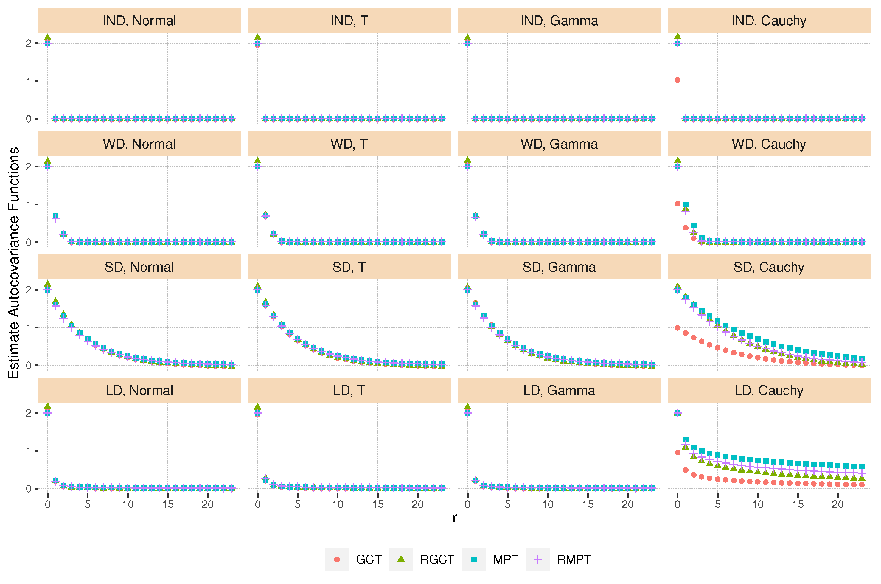
4. Simulation
4.1. Simulation Design
- Normal:
- standard normal distribution Normal (0, 1);
- T:
- t distribution with degrees of freedom 3;
- Gamma:
- centered Gamma distribution with shape parameter 4 and scale parameter 2;
- Cauchy:
- Cauchy (0, 0.1) distribution.
- IND
- (independent): is independently drawn from the innovation distribution for .
- WD
- (weakly dependent): is generated, according to ARMA(2, 2), with autoregressive parameter and moving-average parameters .
- SD
- (strongly dependent): is generated, according to AR(1), with autoregressive parameters .
- LD
- (long-range dependent): Let , where , for constant self-similarity parameters and . Decompose A by Cholesky factorization, to get the matrix U, such that . Independently, draw from the innovation distribution for . Let and set .
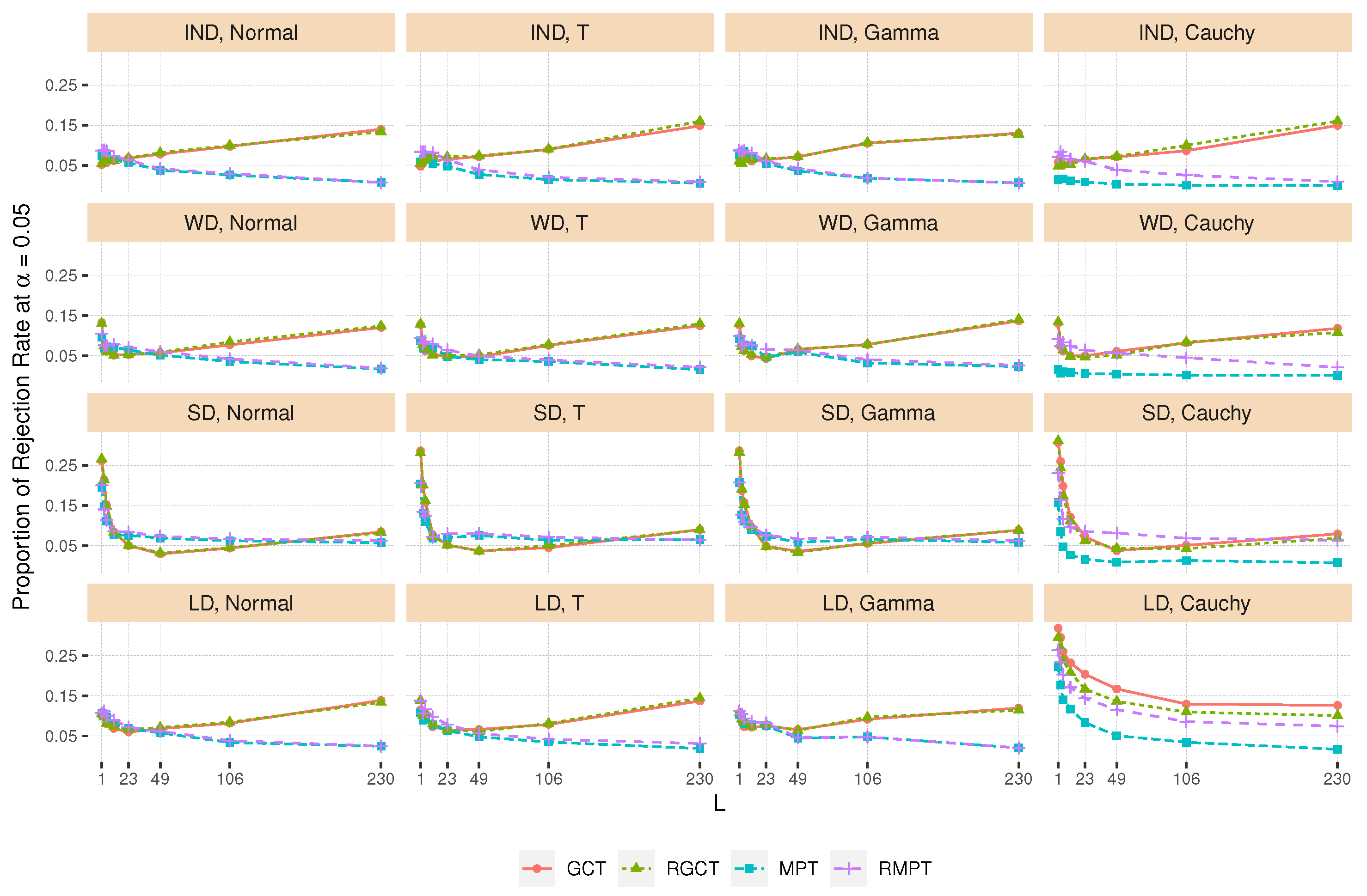
4.2. Adaptive Selection of Window Width L
| Algorithm 1: Data adaptive window width selection |
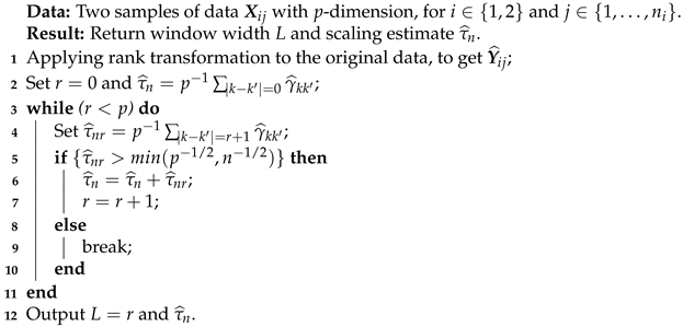 |
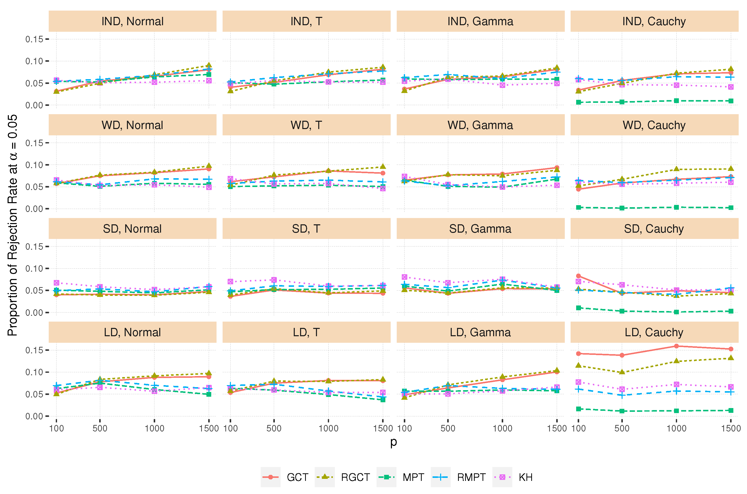
4.3. Type I Error Rate
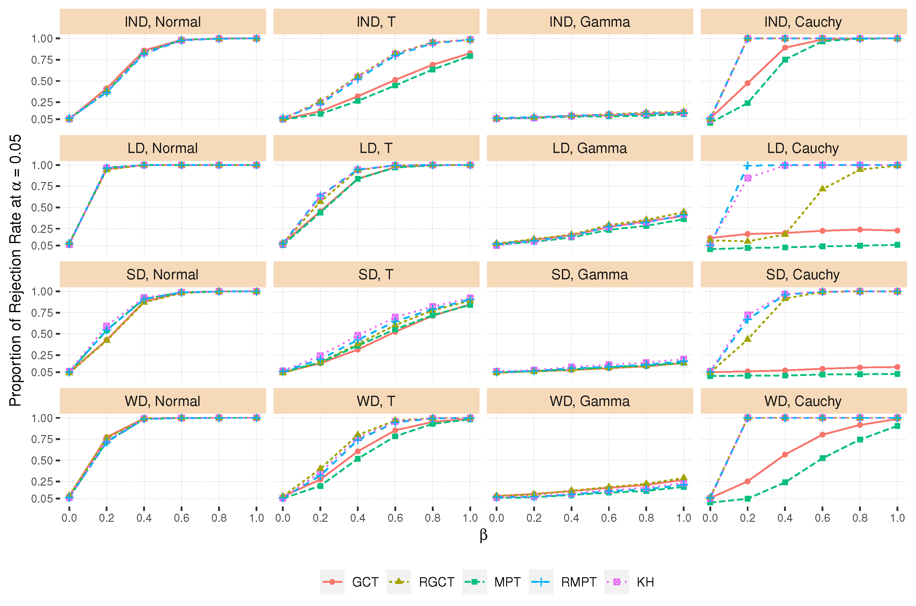
4.4. Power Comparison
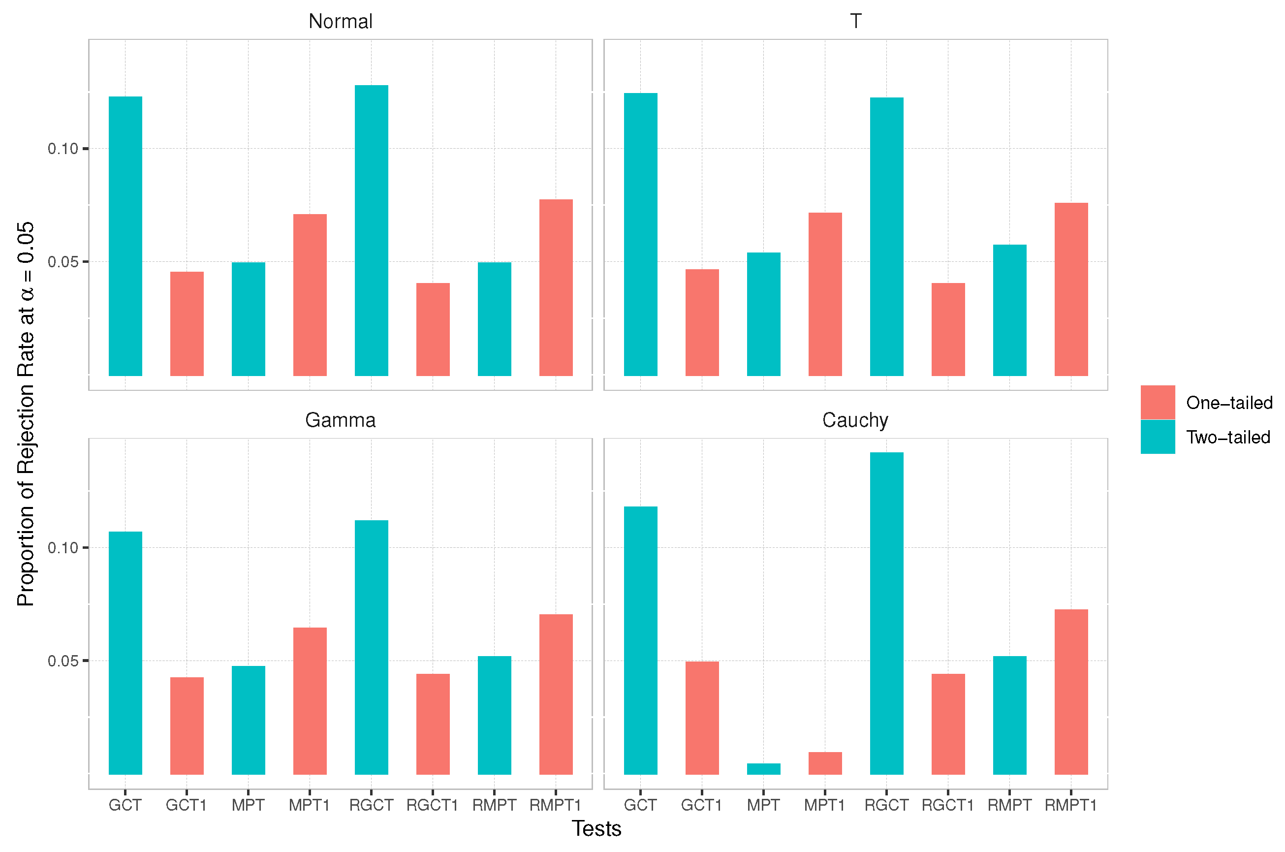
4.5. One-Tailed versus Two-Tailed Tests
5. Conclusions
Author Contributions
Funding
Institutional Review Board Statement
Informed Consent Statement
Data Availability Statement
Acknowledgments
Conflicts of Interest
Appendix A
References
- Harrar, S.W.; Kong, X. Recent developments in high-dimensional inference for multivariate data: Parametric, semiparametric and nonparametric approaches. J. Multivar. Anal. 2022, 188, 104855. [Google Scholar] [CrossRef]
- Anderson, T.W. An Introduction to Multivariate Statistical Analysis, 3rd ed.; Wiley Series in Probability and Statistics; Wiley-Interscience: Hoboken, NJ, USA, 2003. [Google Scholar]
- Bai, Z.; Saranadasa, H. Effect of high dimension: By an example of a two sample problem. Stat. Sin. 1996, 6, 311–329. [Google Scholar]
- Brunner, E.; Munzel, U. The nonparametric Behrens-Fisher problem: Asymptotic theory and a small sample approximation. Biom. J. 2000, 42, 17–25. [Google Scholar] [CrossRef]
- Brunner, E.; Munzel, U.; Puri, M.L. The multivariate nonparametric Behrens-Fisher problem. J. Stat. Plan. Inference 2002, 108, 37–53. [Google Scholar] [CrossRef]
- Brunner, E.; Konietschke, F.; Pauly, M.; Puri, M.L. Rank-based procedures in factorial designs: Hypotheses about non-parametric treatment effects. J. R. Stat. Soc. Ser. B 2017, 79, 1463–1485. [Google Scholar] [CrossRef] [Green Version]
- Konietschke, F.; Aguayo, R.R.; Staab, W. Simultaneous inference for factorial multireader diagnostic trials. Stat. Med. 2018, 37, 28–47. [Google Scholar] [CrossRef]
- Dobler, D.; Friedrich, S.; Pauly, M. Nonparametric MANOVA in meaningful effects. Ann. Inst. Stat. Math. 2020, 72, 997–1022. [Google Scholar] [CrossRef]
- Bathke, A.C.; Harrar, S.W. Nonparametric methods in multivariate factorial designs for large number of factor levels. J. Stat. Plan. Inference 2008, 138, 588–610. [Google Scholar] [CrossRef]
- Harrar, S.W.; Bathke, A.C. Nonparametric methods for unbalanced multivariate data and many factor levels. J. Multivar. Anal. 2008, 99, 1635–1664. [Google Scholar] [CrossRef] [Green Version]
- Bathke, A.C.; Harrar, S.W.; Madden, L.V. How to compare small multivariate samples using nonparametric tests. Comput. Stat. Data Anal. 2008, 52, 4951–4965. [Google Scholar] [CrossRef]
- Burchett, W.W.; Ellis, A.R.; Harrar, S.W.; Bathke, A.C. Nonparametric inference for multivariate data: The R package npmv. J. Stat. Softw. 2017, 76, 1–18. [Google Scholar] [CrossRef] [Green Version]
- Bathke, A.C.; Harrar, S.W. Rank-based inference for multivariate data in factorial designs. In Robust Rank-BASED and Nonparametric Methods; Springer: Berlin, Germany, 2016; pp. 121–139. [Google Scholar]
- Wang, H.; Akritas, M.G. Rank test for heteroscedastic functional data. J. Multivar. Anal. 2010, 101, 1791–1805. [Google Scholar] [CrossRef] [Green Version]
- Kong, X.; Harrar, S.W. High-dimensional rank-based inference. J. Nonparametr. Stat. 2020, 32, 294–322. [Google Scholar] [CrossRef]
- Ruymgaart, F.H. Statistique non Paramétrique Asymptotique: A Unified Approach to the Asymptotic Distribution Theory of Certain Midrank Statistics; Springer: Berlin/Heidelberg, Germany, 1980; pp. 1–18. [Google Scholar]
- Akritas, M.G.; Brunner, E. A unified approach to rank tests for mixed models. J. Stat. Plan. Inference 1997, 61, 249–277. [Google Scholar] [CrossRef]
- Brunner, E.; Munzel, U.; Puri, M.L. Rank-score tests in factorial designs with repeated measures. J. Multivar. Anal. 1999, 70, 286–317. [Google Scholar] [CrossRef] [Green Version]
- Gregory, K.B.; Carroll, R.J.; Baladandayuthapani, V.; Lahiri, S.N. A two-sample test for equality of means in high dimension. J. Am. Stat. Assoc. 2015, 110, 837–849. [Google Scholar] [CrossRef]
- Zhang, H.; Wang, H. A more powerful test of equality of high-dimensional two-sample means. Comput. Stat. Data Anal. 2021, 164, 107318. [Google Scholar] [CrossRef]
- Srivastava, M.S.; Du, M. A test for the mean vector with fewer observations than the dimension. J. Multivar. Anal. 2008, 99, 386–402. [Google Scholar] [CrossRef] [Green Version]
- Srivastava, M.S.; Katayama, S.; Kano, Y. A two sample test in high dimensional data. J. Multivar. Anal. 2013, 114, 349–358. [Google Scholar] [CrossRef]
- Brockwell, P.J.; Davis, R.A. Time Series: Theory and Methods; Springer Series in Statistics; Springer: New York, NY, USA, 2013. [Google Scholar]
- Politis, D.N.; Romano, J.P. Bias-corrected nonparametric spectral estimation. J. Time Ser. Anal. 1995, 16, 67–103. [Google Scholar] [CrossRef]
- Xu, G.; Lin, L.; Wei, P.; Pan, W. An adaptive two-sample test for high-dimensional means. Biometrika 2016, 103, 609–624. [Google Scholar] [CrossRef] [PubMed] [Green Version]
- Chen, S.; Li, J.; Zhong, P. Two-sample and ANOVA tests for high dimensional means. Ann. Stat. 2019, 47, 1443–1474. [Google Scholar] [CrossRef] [Green Version]
- Kong, X.; Harrar, S.W. High-dimensional MANOVA under weak conditions. Stat. A J. Theor. Appl. Stat. 2021, 55, 321–349. [Google Scholar] [CrossRef]
- Bradley, R.C. Basic properties of strong mixing conditions. A Survey and some open questions. Probab. Surv. 2005, 2, 107–144. [Google Scholar] [CrossRef] [Green Version]
- Hall, P.; Jing, B.; Lahiri, S. On the sampling window method for long-range dependent data. Stat. Sin. 1998, 8, 1189–1204. [Google Scholar]
- Samorodnitsky, G. Long Range Dependence; Now Publishers Inc.: Hanover, MA, USA, 2007. [Google Scholar]
Publisher’s Note: MDPI stays neutral with regard to jurisdictional claims in published maps and institutional affiliations. |
© 2022 by the authors. Licensee MDPI, Basel, Switzerland. This article is an open access article distributed under the terms and conditions of the Creative Commons Attribution (CC BY) license (https://creativecommons.org/licenses/by/4.0/).
Share and Cite
Kong, X.; Villasante-Tezanos, A.; Harrar, S.W. Generalized Nonparametric Composite Tests for High-Dimensional Data. Symmetry 2022, 14, 1153. https://doi.org/10.3390/sym14061153
Kong X, Villasante-Tezanos A, Harrar SW. Generalized Nonparametric Composite Tests for High-Dimensional Data. Symmetry. 2022; 14(6):1153. https://doi.org/10.3390/sym14061153
Chicago/Turabian StyleKong, Xiaoli, Alejandro Villasante-Tezanos, and Solomon W. Harrar. 2022. "Generalized Nonparametric Composite Tests for High-Dimensional Data" Symmetry 14, no. 6: 1153. https://doi.org/10.3390/sym14061153