Generic Modeling Method of Quasi-One-Dimensional Flow for Aeropropulsion System Test Facility

Abstract

To support the advanced controller design and verification of the Aeropropulsion System Test Facility (ASTF), it is necessary to establish a mathematical model of ASTF with high precision and replace the current lumped parameter model. Therefore, a quasi-one-dimensional flow model of ASTF is established considering friction, localized losses, heat transfer, etc. Moreover, a generic modeling method is proposed for quasi-one-dimensional flow. With this method, all component models of ASTF are composed of staggered central control volume (CCV) and boundary control volume (BCV) and connected through virtual control volume. Thus, the properties of quasi-one-dimensional flow, such as spatial effect and time delay, can be easily addressed during the modeling process. The simulation results show that the quasi-one-dimensional flow model has higher accuracy than the lumped parameter model. Comparing the simulation results of the quasi-one-dimensional flow model with the test data, the relative errors of flow and pressure are less than 2.2% and 1.4%, respectively, further verifying the correctness of the proposed modeling method.

1. Introduction

By providing airflow at pressures and temperatures experienced during flight, Aeropropulsion System Test Facility (ASTF) can simulate flight conditions to test aircraft engines [1,2]. To simulate more realistic flight conditions, a lot of research on the controller of ASTF is required, which relies on reliable numerical simulation verification. Hence, it is necessary to establish a high-precision numerical simulation model of ASTF.

In fact, ASTF is a symmetrical large-scale pipeline system, including pipe, valve, mixer, flow deflector, air source, etc. As early as 1998, Schmidt et al. [3] proposed a simplified volume model for the pipe, which was obtained from the mass and energy balance. After that, Montgomer et al. [4,5] and Sheeley et al. [6] used the lumped parameter method to develop the math models of test facilities at the Arnold Engineering Development Complex (AEDC), including tanks, pipes, burners, etc. Recently, considering the flow characteristics of the valve and the dynamic characteristics of the volume, Pei et al. [7] established a mathematical model of ASTF. To further improve the accuracy of the ASTF model, Zhu et al. [8] proposed a multi-volume modeling method, which considered the effects of many factors, such as pressure loss of pipeline and fluid–solid heat transfer. The above studies were essentially based on the lumped parameter method, which assumes that the airflow in pipeline is instantaneously mixed evenly and has uniform properties [6]. However, the lumped parameter model cannot directly account for spatial effects and any losses due to friction, bending, etc. [6,9]. It also cannot reflect some important characteristics of ASTF, such as time delay. In addition, the fluid network method [10,11,12] is often used in the research of complex pipeline system, such as natural gas transportation system, engine fuel system, compressed air supply system, etc. It mainly calculates the pressure of each node of the pipeline system and does not care about the flow process inside the pipeline. It is difficult to consider the heat transfer of pipes and other components.

While ensuring high computational efficiency, the one-dimensional (strictly, quasi-one-dimensional) flow method is gradually being studied to improve model accuracy. Pei et al. [13] built a model of the flight environment simulation system, which required that the cavity only be connected with the throttling element. To capture the transient response of the wind tunnel, which is a special pipeline system, Rennie et al. [14] divided the tunnel circuit into small sections, and applied the mass, momentum, and energy conservation equations for each section. However, this model was not suitable for the case that the pipeline has branches. Liu et al. [15,16] established the finite elements state-space model for one-dimensional compressible fluid flow but did not study the model of throttling elements (e.g., control valve). After that, Boylston [9] studied the quasi-one-dimensional flow modeling method for AEDC’s four-foot transonic wind tunnel, but it was still limited to pipe modeling. Inspired by their work, this paper introduces the quasi-one-dimensional flow method into the modeling of ASTF. However, due to the complexity of ASTF’s equipment, models of large valve, mixer, pipe junction, etc., also need to be established. More importantly, previous studies lack a generic modular modeling method for all ASTF’s components. Thus, a generic quasi-one-dimensional flow modeling method of ASTF is proposed. This method makes all component models consist of control volumes. Because the control volume considers heat transfer, friction, local pressure losses and other factors, these factors can be easily introduced into all component models to improve them. In addition, these component models are symmetrical, which facilitates the construction of the system-level model.

The main contributions of this paper are as follows:

(1)

The concepts of CCV, BCV and virtual control volume are proposed, and a generic quasi-one-dimensional flow modeling method is established.

(2)

All the component models and system-level model of ASTF are established, and the limitation that the cavity can only be connected with the throttling element is eliminated.

This paper is organized as follows. In Section 2, two basic control volumes as well as the calculation methods of parameters are introduced, serving as the backbone for the modeling framework. In Section 3, through the staggered connection of CCV and BCV, the component models of ASTF are constructed, including the pipeline model, control valve model, multi-port junction model, flow source/sink model and pressure/temperature boundary model. To unify the boundary of the component models and build the system-level model, the virtual control volume is proposed as the connection of models. Section 4 presents the characteristics and establishment method of the system-level model, and then constructs a numerical simulation model of ASTF. Section 5 describes the differences between the quasi-one-dimensional flow model and lumped parameter model in steady-state and dynamic processes. By comparing the simulation results with test data, the correctness of the modeling method proposed in this paper is further verified. Section 6 provides concluding remarks.

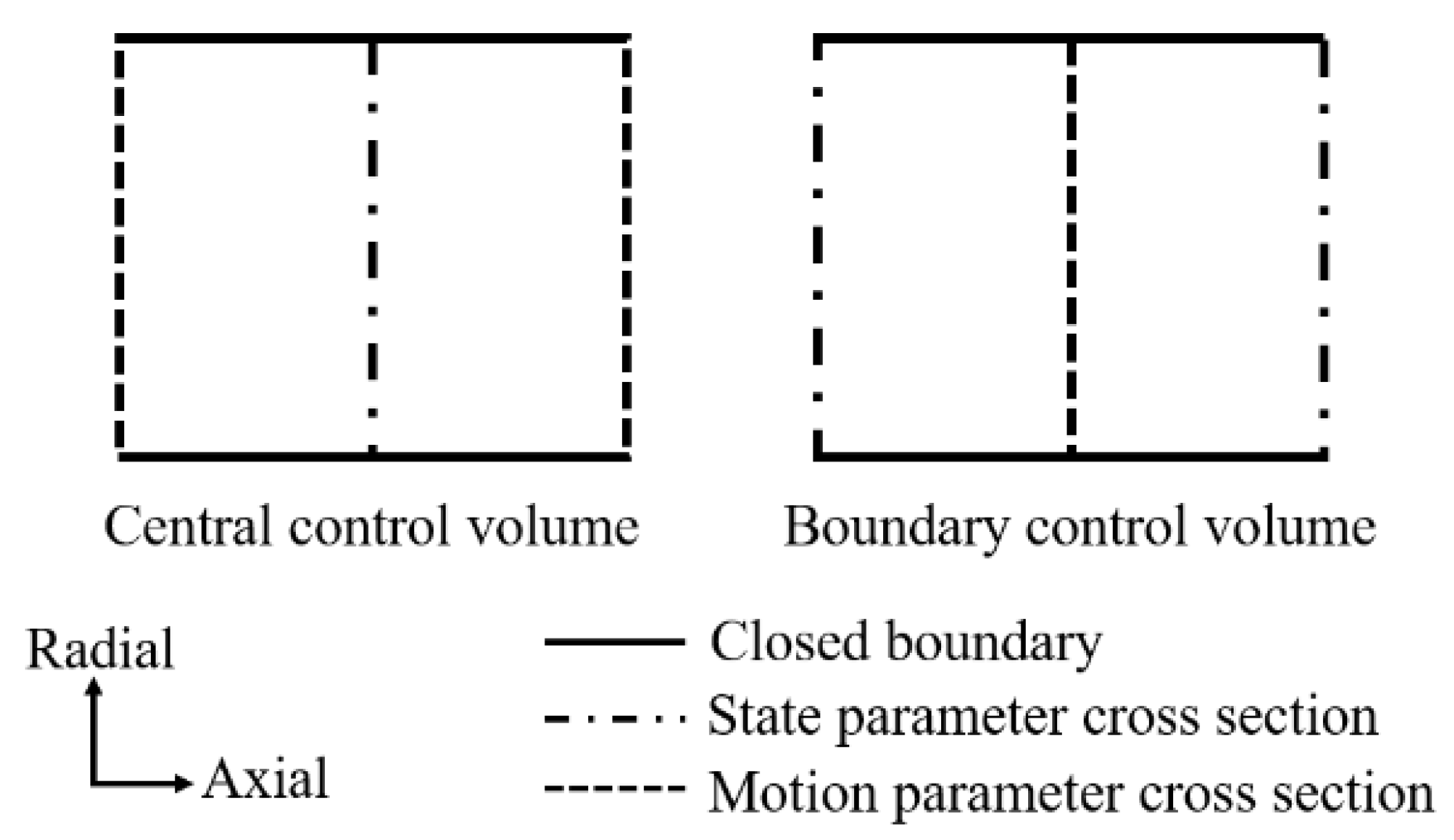
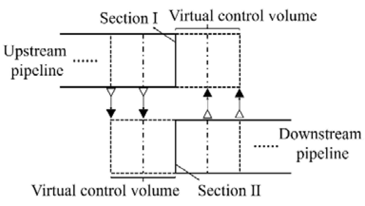
2. Control Volume

Assumptions:

• The fluid in control volume is instantaneously mixed evenly and has uniform properties.
• The gravitational potential energy is ignored.

According to the difference of the concerned sections, control volumes are classified into two types: central control volume (CCV) and boundary control volume (BCV), as shown in Figure 1. The temperature, pressure, density and energy of the fluid are calculated in the state parameter cross section. The velocity, momentum and Mach number of the fluid are calculated in the motion parameter cross section. The boundary of the CCV is the motion parameter cross section, while the boundary of BCV is the state parameter cross section. The fluid moves only along the axial direction, and the radial boundary is closed. Although the parameters of each section can be calculated in different ways, the basic conservation equation is mostly used, which is briefly reviewed in the following.

2.1. Central Control Volume

As shown in Figure 2, it is assumed that the boundary parameters of CCV are known. According to the mature theory of unsteady flow of compressible fluid [9,17,18], the parameters of the CCV’s state parameter cross section can be calculated as follows:

$$\frac{\mathrm{d}\left({\rho }_j{V}_j\right)}{\mathrm{d}t}={\rho }_{\mathrm{in}}{v}_i{A}_i-{\rho }_{\mathrm{out}}{v}_i{A}_i$$

(1)

$$\frac{\mathrm{d}\left(E_j{\rho }_j{V}_j\right)}{\mathrm{d}t}=\left(E_{\mathrm{in}}+\frac{p_{\mathrm{in}}}{{\rho }_{\mathrm{in}}}\right){\rho }_{\mathrm{in}}{v}_i{A}_i-\left(E_{\mathrm{out}}+\frac{p_{\mathrm{out}}}{{\rho }_{\mathrm{out}}}\right){\rho }_{\mathrm{out}}{v}_{i+1}{A}_{i+1}+{\dot{Q}}_j-\dot{\Psi }$$

(2)

where $V_j$ is the volume of CCV. The subscript i + 1 represents the downstream motion parameter section adjacent to motion parameter section i. $E_{\mathrm{in}}$, $p_{\mathrm{in}}$, ${\rho }_{\mathrm{in}}$, $E_{\mathrm{out}}$, $p_{\mathrm{out}}$ and ${\rho }_{\mathrm{out}}$ need to be calculated according to the parameters of adjacent upstream and downstream grids, such as taking the average value [9] or upwind scheme [19] (see Section 3.1 for details). Equation (1) represents the conservation of mass, that is,

$$\left(\begin{array}{c}\begin{array}{c}\mathrm{Time} \mathrm{rate} \mathrm{of} \mathrm{change} \\ \mathrm{of} \mathrm{mass} \mathrm{within} \mathrm{the} \mathrm{CCV}\end{array}\end{array}\right)=\left(\begin{array}{c}\mathrm{Total} \mathrm{mass} \mathrm{flow} \mathrm{rate} \\ \mathrm{entering} \mathrm{the} \mathrm{CCV}\end{array}\right)-\left(\begin{array}{c}\mathrm{Total} \mathrm{mass} \mathrm{flow} \mathrm{rate}\\ \mathrm{leaving} \mathrm{the} \mathrm{CCV}\end{array}\right)$$

Equation (2) represents the conservation of energy, that is,

$$\begin{array}{ll}\left(\begin{array}{c}\mathrm{Time} \mathrm{rate} \mathrm{of} \mathrm{change} \mathrm{of} \\ \mathrm{total} \mathrm{energy} \mathrm{within} \mathrm{the} \mathrm{CCV}\end{array}\right)& =\left(\begin{array}{c}\mathrm{Rate} \mathrm{of} \mathrm{energy} (\mathrm{transferred}\\ \mathrm{by} \mathrm{mass}) \mathrm{entering} \mathrm{the} \mathrm{CCV}\end{array}\right)\\ & -\left(\begin{array}{c}\mathrm{Rate} \mathrm{of} \mathrm{energy} (\mathrm{transferred}\\ \mathrm{by} \mathrm{mass}) \mathrm{leaving} \mathrm{the} \mathrm{CCV}\end{array}\right)+\left(\begin{array}{c}\mathrm{Rate} \mathrm{of} \mathrm{net}\\ \mathrm{heat} \mathrm{input}\end{array}\right)-\left(\begin{array}{c}\mathrm{Rate} \mathrm{of} \mathrm{net}\\ \mathrm{work} \mathrm{output}\end{array}\right)\end{array}$$

In Equation (2), ${\dot{Q}}_j=h{A}_s(T_{\mathrm{pipe}}-T_j)$, and $A_s$ is the surface area through which the convection heat transfer takes place, $T_{\mathrm{pipe}}$ is the wall temperature, and $T_j$ is the temperature of the airflow in CCV [20,21]. Actually, $h$ can be variable, and detailed calculation can be found in Refs. [9,22,23]. For ASTF, the fluid does not do shaft work, so ${\Psi }_s=0$. Since the radial boundary of the control volume is a solid wall, where the velocity of the fluid is zero, the work done by the viscous force is zero. Then, $\Psi ={\Psi }_s+{\Psi }_v=0$.

According to the state equation for ideal gas and the relationship between internal energy and state parameters, the pressure in the state parameter cross section can be obtained as [24]

$$p_j=\left(\gamma -1\right){\rho }_j\left[E_j-\frac{1}{2}{v}_j^2\right]$$

(3)

where $v_j\approx \frac{1}{2}\left(v_i+v_{i+1}\right)$.

2.2. Boundary Control Volume

As shown in Figure 3, it is assumed that the boundary parameters of BCV are known. According to the mature theory of the unsteady flow of compressible fluid [9,17,18], the parameters of BCV’s motion parameter cross section can be calculated as follows:

$$\frac{\mathrm{d}{W}_i}{\mathrm{d}t}=\left(p_{j-1}{A}_{j-1}-p_j{A}_j+p_i{A}_j-p_i{A}_{j-1}\right)+{\rho }_{j-1}{v}_{\mathrm{in}}^2{A}_{j-1}-{\rho }_j{v}_{\mathrm{out}}^2{A}_j-\frac{V_i{\rho }_{i}f}{2D_i}{v}_i\left|v_i\right|-\frac{A_i{\rho }_{i}k}{2}{v}_i\left|v_i\right|$$

(4)

where $v_{\mathrm{in}}$ and $v_{\mathrm{out}}$ also need to be approximated (see Section 3.1 for details). The subscript j-1 represents the upstream state parameter section adjacent to state parameter section j. $p_i\approx \frac{1}{2}\left(p_{j-1}+p_j\right)$ and ${\rho }_i\approx \frac{1}{2}\left({\rho }_{j-1}+{\rho }_j\right)$ are state parameters of the motion parameter cross section. Equation (4) represents the conservation of momentum, that is,

$$\begin{array}{ll}\left(\begin{array}{c}\mathrm{Time} \mathrm{rate} \mathrm{of} \mathrm{change} \mathrm{of}\\ \mathrm{momentum} \mathrm{within} \mathrm{the} \mathrm{CCV}\end{array}\right)& =\left(\begin{array}{c}\mathrm{Force} \mathrm{on} \mathrm{the} \mathrm{fluid}\\ \mathrm{due} \mathrm{to} \mathrm{pressure}\end{array}\right)+\left(\begin{array}{c}\mathrm{The} \mathrm{rate} \mathrm{of} \mathrm{change} \mathrm{of} \mathrm{momentum}\\ \mathrm{brought} \mathrm{in} \mathrm{by} \mathrm{the} \mathrm{incoming} \mathrm{fluid}\end{array}\right)\\ & -\left(\begin{array}{c}\mathrm{The} \mathrm{rate} \mathrm{of} \mathrm{change} \mathrm{of} \mathrm{momentum}\\ \mathrm{leaving} \mathrm{with} \mathrm{the} \mathrm{outgoing} \mathrm{fluid}\end{array}\right)\\ & -\left(\begin{array}{c}\mathrm{Frictional} \mathrm{force}\\ \mathrm{acting} \mathrm{against} \mathrm{the} \mathrm{flow}\end{array}\right)-\left(\mathrm{Force} \mathrm{due} \mathrm{to} \mathrm{minor} \mathrm{pressure} \mathrm{losses}\right)\end{array}$$

By introducing $f$ and $k$ into Equation (4), the subsequent model can handle a variety of situations, such as friction, bends, flow obstructions, etc. For laminar flow (i.e., $\mathrm{Re}\le 2400$), the friction factor $f$ can be approximated by $64/\mathrm{Re}$. When $\mathrm{Re}>2400$, the friction factor $f$ can be approximated by $0.25/{\left[\log \left(\frac{\epsilon }{3.7D}+\frac{5.74}{{\mathrm{Re}}^{0.9}}\right)\right]}^2$ [9]. The minor loss coefficient $k$ is related to the structure of local obstacles and the actual pipeline, which is usually determined by experiments. The detailed description of $k$ can be found in Refs. [9,25].

According to the definition of momentum, the velocity in the motion parameter cross section is obtained as

$$v_i=\frac{W_i}{{\rho }_i{V}_i}$$

(5)

2.3. Outlook

CCV and BCV deal with parameters of different cross sections, and thus the one-dimensional flow process can be calculated by the staggered connection of CCV and BCV. Although this method is essentially similar to the one-dimensional flow in previous studies, this description method in this paper gives more convenience and universality to subsequent modeling. Any component and even the whole system can be described by the staggered connection of CCV and BCV, not limited to the pipeline.

The control volumes contain the parameters of different cross sections. In addition to the above calculation methods, for different components, their parameters are allowed to be calculated by different equations (see Section 3.2). Some parameters of the control volumes are unknown, which will be considered in the component modeling.

3. Component Models

As a pipeline system, the parameter distribution along the axial direction reflects the main characteristics of ASTF. Therefore, the difference of the radial parameters of airflow is ignored, and only the one-dimensional flow of the airflow in the pipeline system is considered. Based on this, the pipeline, control valve, multi-port junction, flow source/sink, pressure/temperature boundary and other components can be equivalent to the combination of CCV and BCV. Since the structure of each model is symmetrical, the direction of airflow does not affect the calculation of the model. Except for the flow source/sink model, which has a definite flow direction, the other models only need a default flow direction.

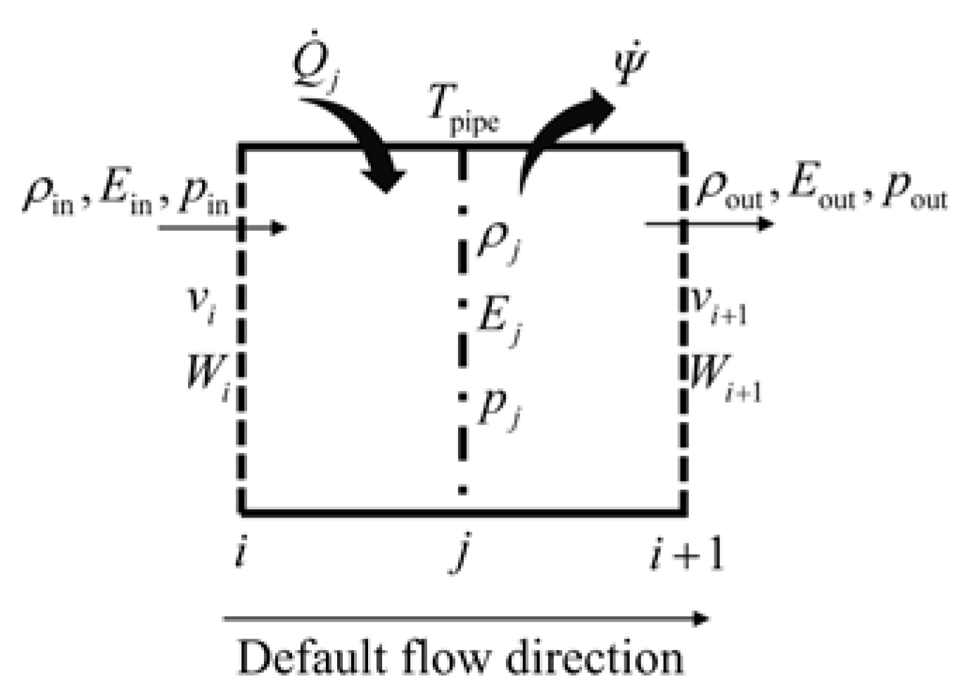
3.1. Pipeline Model

Based on the staggered grid, a one-dimensional flow model can be established [9,16,19,24]. Here, the CCV and BCV are staggered together to form a one-dimensional pipeline model, as shown in Figure 4. In the figure, the black triangle represents the input port, and the white triangle represents the output port. The subscript j + 1 represents the downstream state parameter section adjacent to state parameter section j. The subscript i-1 represents the upstream motion parameter section adjacent to motion parameter section i.

The unknown state parameters can be calculated using the upwind scheme, and the unknown motion parameters can be approximated by the average value, as shown in Equations (6) and (7).

$$y_{\mathrm{in}}=\{\begin{array}{l}{y}_{j-1},v_i\ge 0\hfill \\ y_j,v_i<0\hfill \end{array}\hspace{1em},\hspace{1em}{y}_{\mathrm{out}}=\{\begin{array}{l}{y}_j,v_i\ge 0\hfill \\ y_{j+1},v_i<0\hfill \end{array}$$

(6)

$$v_{\mathrm{in}}=\frac{1}{2}\left(v_{i-1}+v_i\right)\hspace{1em},\hspace{1em}{v}_{\mathrm{out}}=\frac{1}{2}\left(v_i+v_{i+1}\right)$$

(7)

where $i=1,2,\cdots ,n$ and $y\in \left\{\rho ,E,p\right\}$.

Previous studies have carried out special treatment on the pipeline boundary, generally taking actual physical parameters as boundary conditions. In this paper, two virtual control volumes are set at both ends of the pipeline. The parameters of the virtual control volumes (i.e., the boundary conditions of the pipeline model) are provided by the upstream and downstream ports. Thus, the parameters of each cross section in the pipeline model can be directly calculated according to Equations (1)–(7). The calculation results of the virtual control volumes are returned as the output to the upstream and downstream ports, as shown in Figure 4.

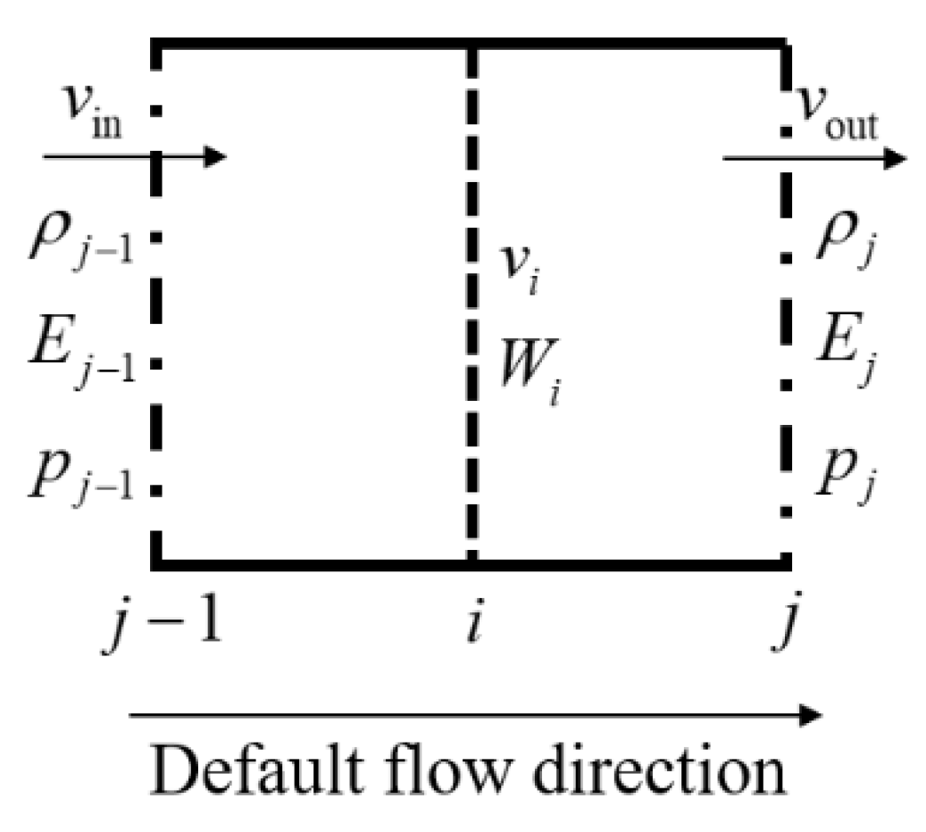
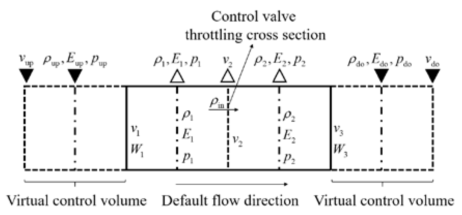
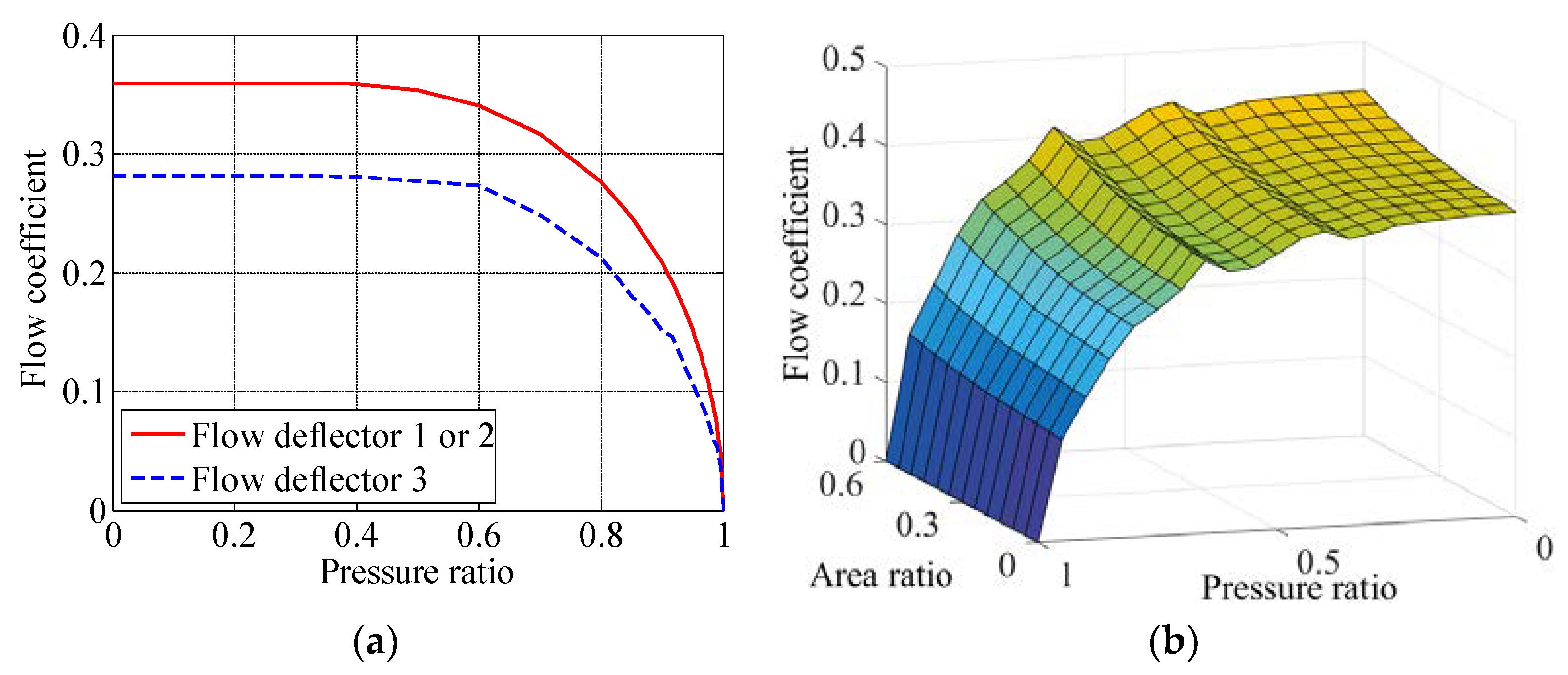
3.2. Control Valve Model

ASTF’s control valve is a large-size throttling component. The dynamic process of the airflow through the control valve directly affects the characteristics of ASTF. The presence of the valve plate makes the contact area between the valve body and airflow large so that the heat transfer process between the control valve and the airflow cannot be ignored. The control valve model can be established through the staggered connection of two CCVs and one BCV, as shown in Figure 5. The two CCVs are located on both sides of the throttling cross section of the control valve, which can reflect the dynamic process of the airflow. Moreover, the heat transfer process can be considered in the two CCVs to simulate the energy change of the airflow through the control valve.

In ASTF, the structure of the large-size control valve is complicated, and it is difficult to establish its flow characteristic model with the traditional theoretical formula [26]. Actually, a large amount of data is retained during the operation of ASTF, which can be used to improve the accuracy of the model. The mass flow rate through the control valve can be written as [27]

$$\dot{m}=\phi S\sqrt{2{\rho }_1{p}_1}$$

(8)

where $\phi =g\left(S,\pi \right)$ is the flow coefficient of control valve, and it is a function of pressure ratio $\pi =p_2/p_1$. g represents a complicated function. Through the fitting of test data and the calibration of the three-dimensional flow field simulation data, an interpolation table of the flow coefficient can be obtained to replace $g$ [28].

The flow velocity at the throttling cross section can be calculated as

$$v_2=\frac{\dot{m}}{{\rho }_{\mathrm{in}}S}$$

(9)

where ${\rho }_{\mathrm{in}}=\{\begin{array}{l}{\rho }_1,\dot{m}\ge 0\hfill \\ {\rho }_2,\dot{m}<0\hfill \end{array}$ is determined by the upwind scheme. The state parameter sections corresponding to subscripts 1 and 2 are shown in Figure 5.

The motion parameters at the throttle cross section are obtained, so Equation (4) is no longer needed. We set the virtual control volumes at both ends of the control valve, and the upstream and downstream ports provide the boundary conditions. According to Equations (1)–(7), the parameters of each section (except the throttle cross section) can be calculated. Then the parameters of BCV are provided to the upstream and downstream ports.

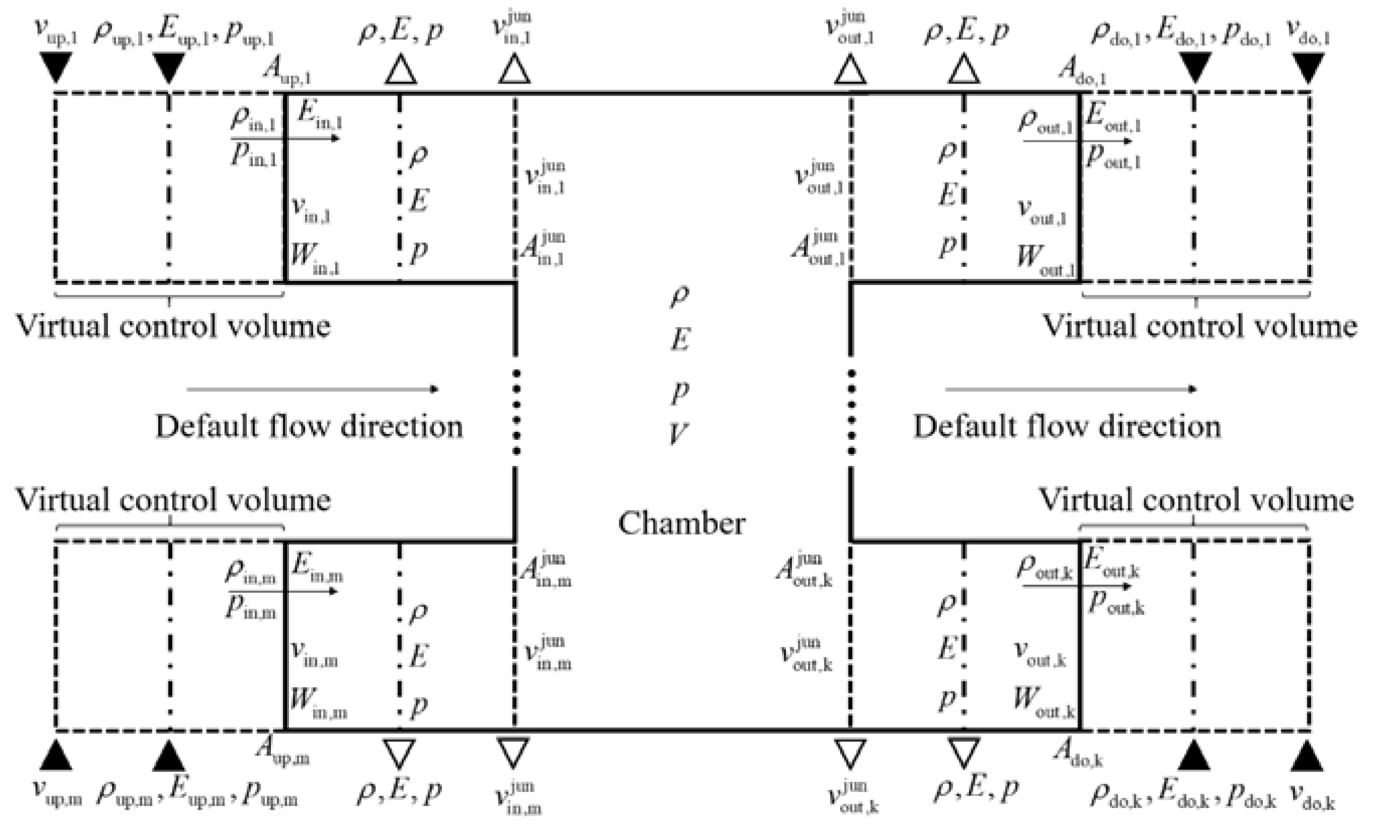
3.3. Multi-Port Junction Model

The multi-port junction model is used for the intersection and branching of pipelines. The schematic diagram of the multi-port junction model with m inlets and k outlets is shown in Figure 6, and the virtual control volumes are also set for each port of the model.

Assuming that the airflow at the pipe junction is uniformly mixed instantaneously, according to Equations (1) and (2), the parameters in the multi-port junction can be calculated as

$$\frac{\mathrm{d}\left(\rho V\right)}{\mathrm{d}t}={\displaystyle \sum _{i=1}^{\mathrm{m}}{\rho }_{\mathrm{in},i}{v}_{\mathrm{up},i}{A}_{\mathrm{up},i}}-{\displaystyle \sum _{j=1}^{\mathrm{k}}{\rho }_{\mathrm{out},j}{v}_{\mathrm{do},j}{A}_{\mathrm{do},j}}$$

(10)

$$\frac{\mathrm{d}\left(E\rho V\right)}{\mathrm{d}t}={\displaystyle \sum _{i=1}^{\mathrm{m}}\left(E_{\mathrm{in},i}+\frac{p_{\mathrm{in},i}}{{\rho }_{\mathrm{in},i}}\right){\rho }_{\mathrm{in},i}{v}_{\mathrm{in},i}{A}_{\mathrm{up},i}}-{\displaystyle \sum _{j=1}^{\mathrm{k}}\left(E_{\mathrm{out},j}+\frac{p_{\mathrm{out},j}}{{\rho }_{\mathrm{out},j}}\right){\rho }_{\mathrm{out},j}{v}_{\mathrm{out},j}{A}_{\mathrm{do},j}}+\dot{Q}-\dot{\Psi }$$

(11)

From Equations (3), (10) and (11), the state parameters $\rho$, $E$, and $p$ of the output ports can be determined. To unify the interface, it is still necessary to calculate the motion parameters of the output ports. Considering that the volume of multi-port junction is concentrated inside, and the control volumes at the inlet and outlet are relatively small, the compressibility of the air in these control volumes can be ignored. Therefore, the velocity of the inlet and outlet airflow can be expressed as follows according to the flow equilibrium,

$$v_{\mathrm{in},i}^{\mathrm{jun}}=\frac{{\rho }_{\mathrm{in},i}{v}_{\mathrm{in},i}{A}_{\mathrm{up},i}}{\rho A_{\mathrm{up},i}^{\mathrm{jun}}},i=1,2,\cdots ,\mathrm{m}$$

(12)

$$v_{\mathrm{out},j}^{\mathrm{jun}}=\frac{{\rho }_{\mathrm{out},j}{v}_{\mathrm{out},j}{A}_{\mathrm{do},j}}{\rho A_{\mathrm{out},j}^{\mathrm{jun}}},j=1,2,\cdots ,\mathrm{k}$$

(13)

In Equations (10)–(13), the state parameters such as ${\rho }_{\mathrm{in},i}$, $E_{\mathrm{in},i}$, $p_{\mathrm{in},i}$, ${\rho }_{\mathrm{out},j}$, $E_{\mathrm{out},j}$, and $p_{\mathrm{out},j}$, are calculated according to the upwind scheme shown in Equation (6), and the motion parameters $v_{\mathrm{in},i}$, $W_{\mathrm{in},i}$, $v_{\mathrm{out},j}$, and $W_{\mathrm{out},j}$, are calculated according to Equations (4) and (5) of BCV, for $i=1,2,\cdots \mathrm{m}$ and $j=1,2,\cdots ,\mathrm{k}$.

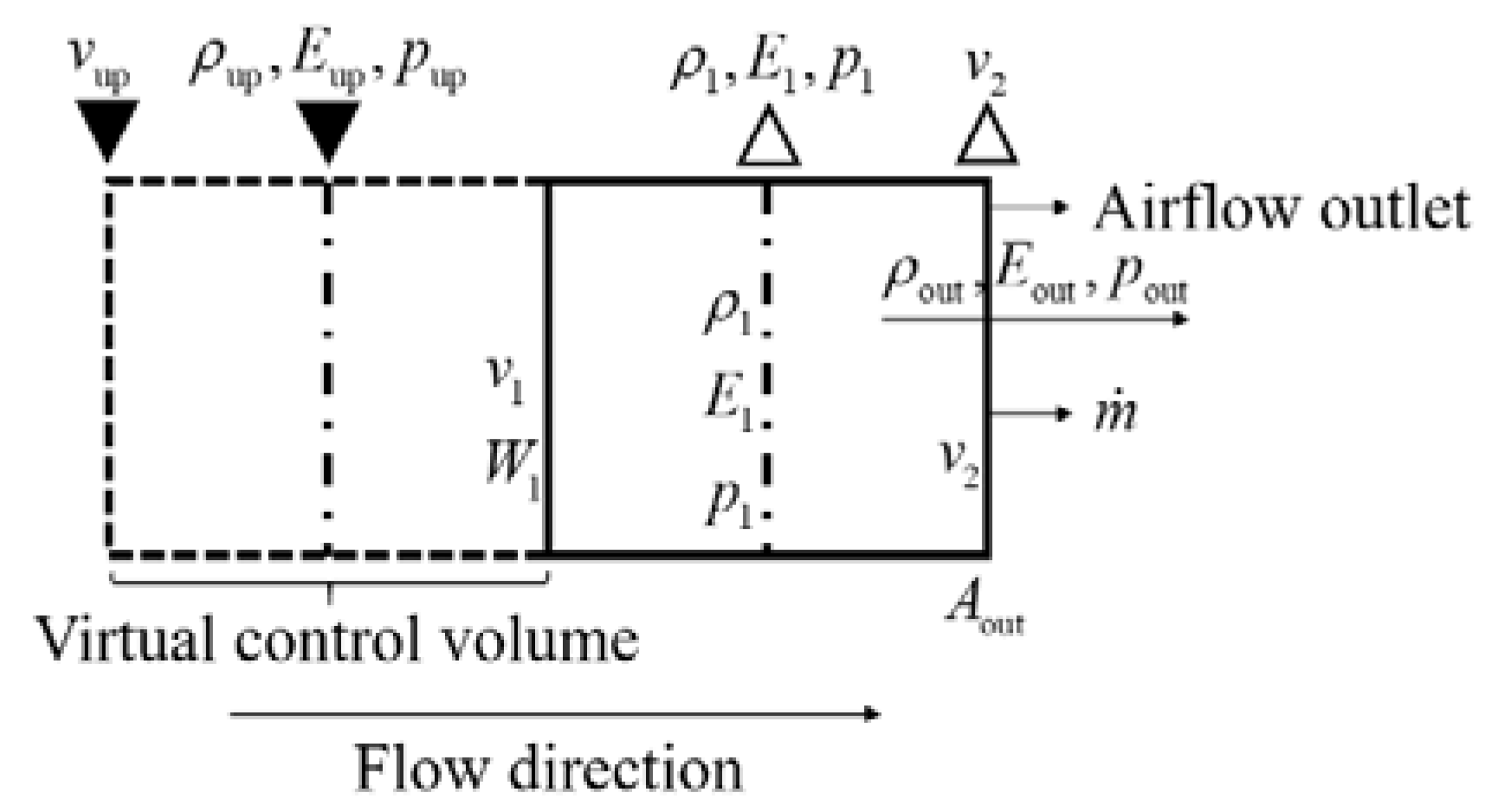
3.4. Flow Source/Sink Model

The flow source model can be used to simulate the air supply unit of ASTF, where the mass flow rate and temperature are known. A single CCV is used as the flow source model, and a virtual control volume is set at its outlet, as shown in Figure 7. Since the virtual control volume is not set at the inlet of the flow source model, the parameters of the entrance section cannot be obtained directly by the upwind scheme. According to the mass flow rate, the entrance velocity is expressed as

$$v_1=\frac{\dot{m}}{{\rho }_{\mathrm{in}}{A}_{\mathrm{in}}}$$

(14)

where the air flow density is approximated as ${\rho }_{\mathrm{in}}\approx {\rho }_1$.

The airflow pressure therefore becomes $p_{\mathrm{in}}={\rho }_{1}RT$. From Equation (3), the total energy $E_{\mathrm{in}}$ of inlet air flow can further be determined. Combining Equations (1)–(7), the remaining parameters of the control volume can be solved. The model output port parameters are shown in Figure 7.

The flow sink model can be used to simulate the intake air of an aircraft engine, and a virtual control volume is set at the inlet, as shown in Figure 8. Since the air flow direction is fixed, the state parameters of the exit section can be taken as

$$y_{\mathrm{out}}=y_1$$

(15)

where $y\in \left\{\rho ,E,p\right\}$.

The outlet flow rate is a known value, and then the outlet velocity is expressed as

$$v_2=\frac{\dot{m}}{{\rho }_{\mathrm{out}}{A}_{\mathrm{out}}}$$

(16)

According to Equations (1)–(7), the parameters of the remaining sections can be obtained, and the parameters of output port are shown in Figure 8.

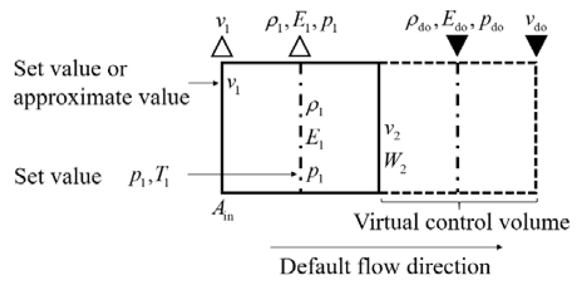
3.5. Pressure/Temperature Boundary Model

The pressure/temperature boundary model represents the known airflow boundary, such as atmospheric environment, etc. In addition to state parameters that can be output as known values, the model still needs to output motion parameters, as shown in Figure 9.

For low-speed flow, kinetic energy accounts for a small proportion of the total energy of the air flow. Therefore, it is allowed to set a reasonable velocity based on experience without causing a large loss of accuracy. When the experience is insufficient or the speed is high, such as close to the air supply unit, it can be approximated as

$$v_1\approx v_2$$

(17)

The state parameters $p_1$ and $T_1$ are known setting values, and the airflow density ${\rho }_1$ and total energy $E_1$ can be calculated according to the ideal gas state equation and Equation (3). In addition, a virtual control volume is added to the model, and the unknown motion parameters $v_2$ and $W_2$ are calculated according to Equations (4) and (5).

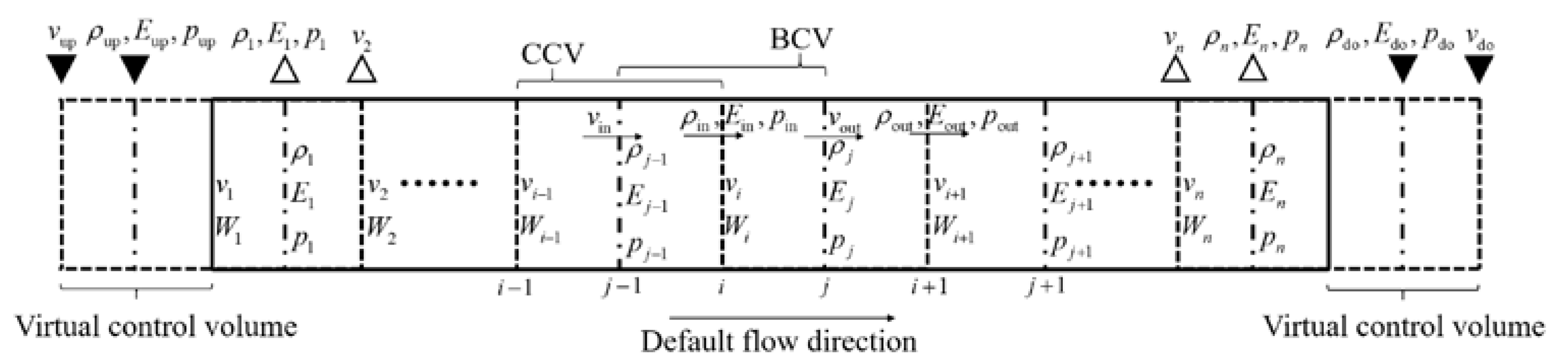
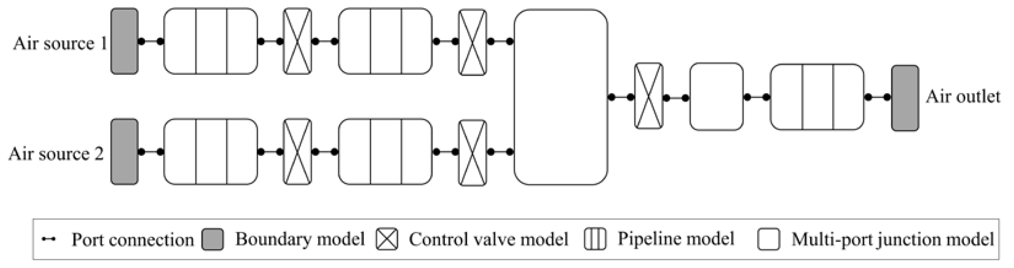
4. System-Level Model

4.1. Analysis of System-Level Modeling

The virtual control volume can conveniently handle model interfaces and boundaries. In Figure 10, the input/output ports of the upstream pipeline are respectively connected to the output/input ports of the downstream pipeline, so that the virtual control volumes essentially become CCVs of the connected pipelines. Then, Section I of the upstream pipeline and Section II of the downstream pipeline are seamlessly connected, and the parameters of the two sections remain the same. Although the pipelines connected in sections can be simplified into a single pipeline model, when the pipeline length reaches hundreds of meters, it is inconvenient to set all the pipeline parameters on one model. In addition, this method does not increase the computational complexity of the model.

Figure 11 shows the connection between the pipeline and the control valve, in which the state parameter cross sections all follow the mass conservation equation and energy conservation equation, and only the calculation method of the motion parameter cross section is different. For the control valve, the motion parameters are calculated based on the mass flow rate through the control valve. For the pipeline, the motion parameters are calculated according to the momentum conservation equation.

Therefore, for the system-level model, it is still in the form of complete staggered grids, in which the motion parameters can be combined with the characteristics of different components for targeted design and calculation. That also determines the flow characteristics of the airflow in ASTF. The characteristics of one-dimensional (strictly, quasi-one-dimensional) flow can be reflected in the whole system model. Due to the symmetry of the component models, the airflow direction in ASTF does not affect the modeling process.

Generally, due to the staggered grids and the average properties of some parameters (e.g., Equation (7)), the quasi-one-dimensional flow model cannot simulate supersonic flow stably and accurately [9]. Although reducing the grid size is a solution, the computational cost is very large because of the larger grid number. However, this does not affect the modeling of ASTF, because the airflow in ASTF is designed to be at a low Mach number.

4.2. ASTF Model

The ASTF structure is shown in Figure 12, which is mainly composed of pipelines, control valves, flow deflectors, mixer, buffer chamber, etc. The structure of ASTF is symmetrical. It regulates the flow of air source through the control valve and realizes the mixing of airflow with different temperatures and pressures in the mixer. After the mixed airflow passes through the buffer chamber and the special-shaped pipe, it is directly supplied to the aircraft engine. The buffer chamber can make the airflow mix more evenly. The special-shaped pipe makes the airflow more stable. A flow tube is used to measure the mass flow rate, temperature, pressure and other parameters. According to the actual structure and system working mechanism, the ASTF model is constructed as shown in Figure 13.

In Figure 13, the boundary model represents the flow source/sink model or pressure/temperature boundary model, which needs to be selected according to the actual boundary type. As a throttling component, the flow deflector is represented by a control valve model with a fixed opening, and its flow coefficient is obtained by fitting three-dimensional flow field simulation data, as shown in Figure 14a. The flow coefficient of the control valve is obtained through test data and three-dimensional flow field simulation data, as shown in Figure 14b. The pressure ratio in Figure 14 represents the ratio of the airflow pressure after and before the control valve, and the area ratio represents the ratio of the valve opening area to the valve maximum cross-sectional area. The mixer has the characteristics of airflow mixing, while the buffer chamber is a typical large-scale volume, and both are modeled by the multi-port junction model. Since some component models are not strictly one-dimensional flow numerical models, the ASTF model is a quasi-one-dimensional flow model.

By setting the boundary model parameters (i.e., temperature/pressure or mass flow rate) and the opening of the control valves, the subsequent simulations can be carried out.

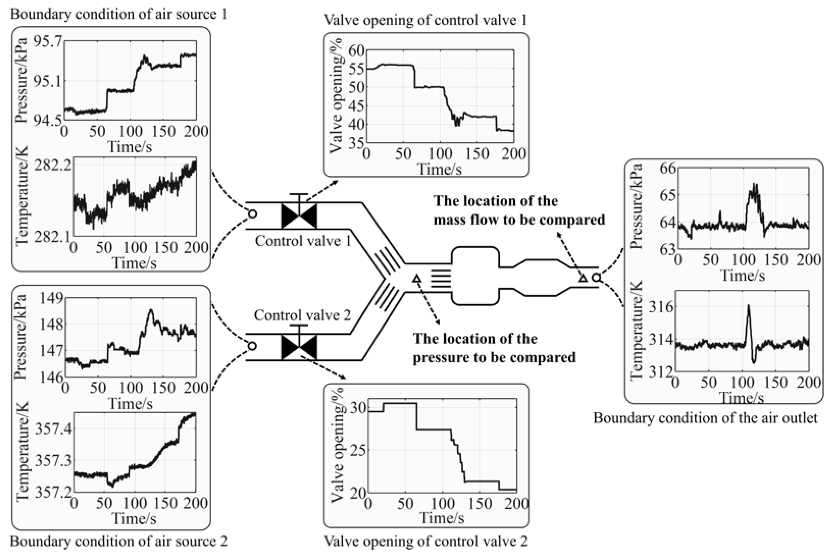
5. Simulation and Analysis

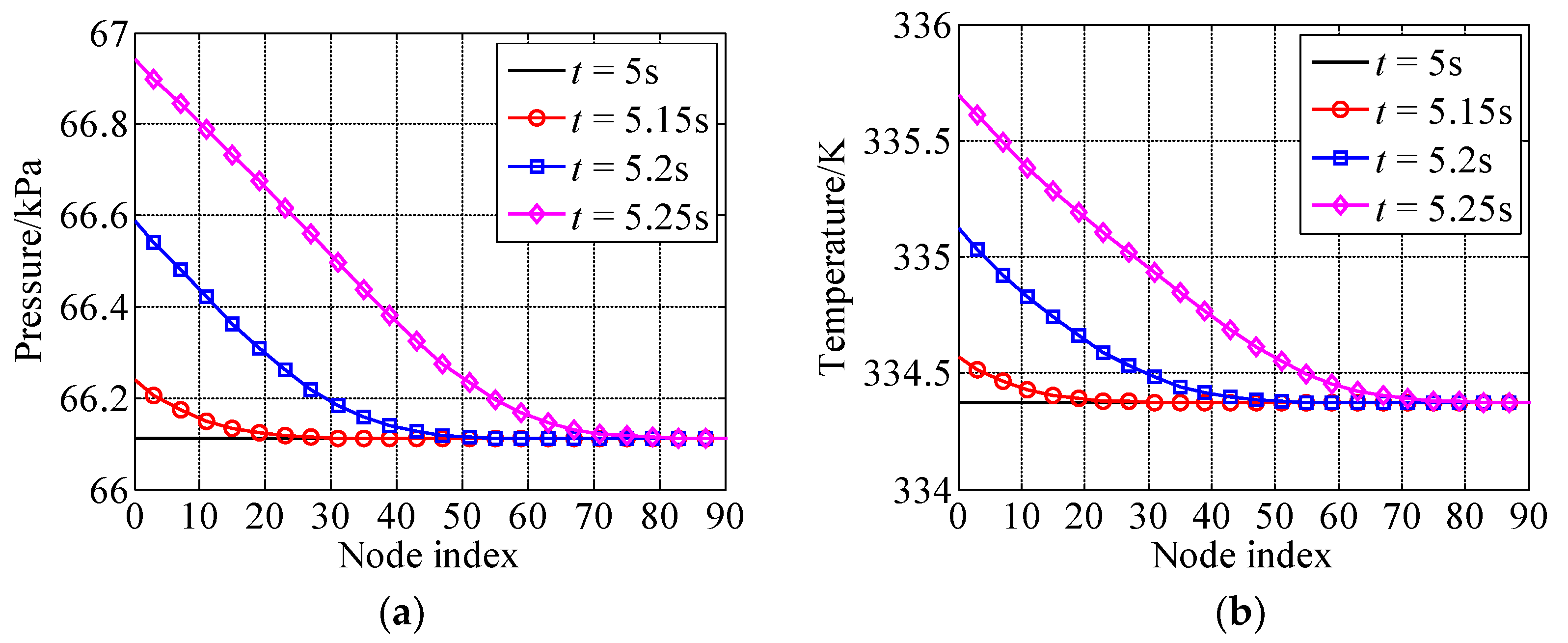
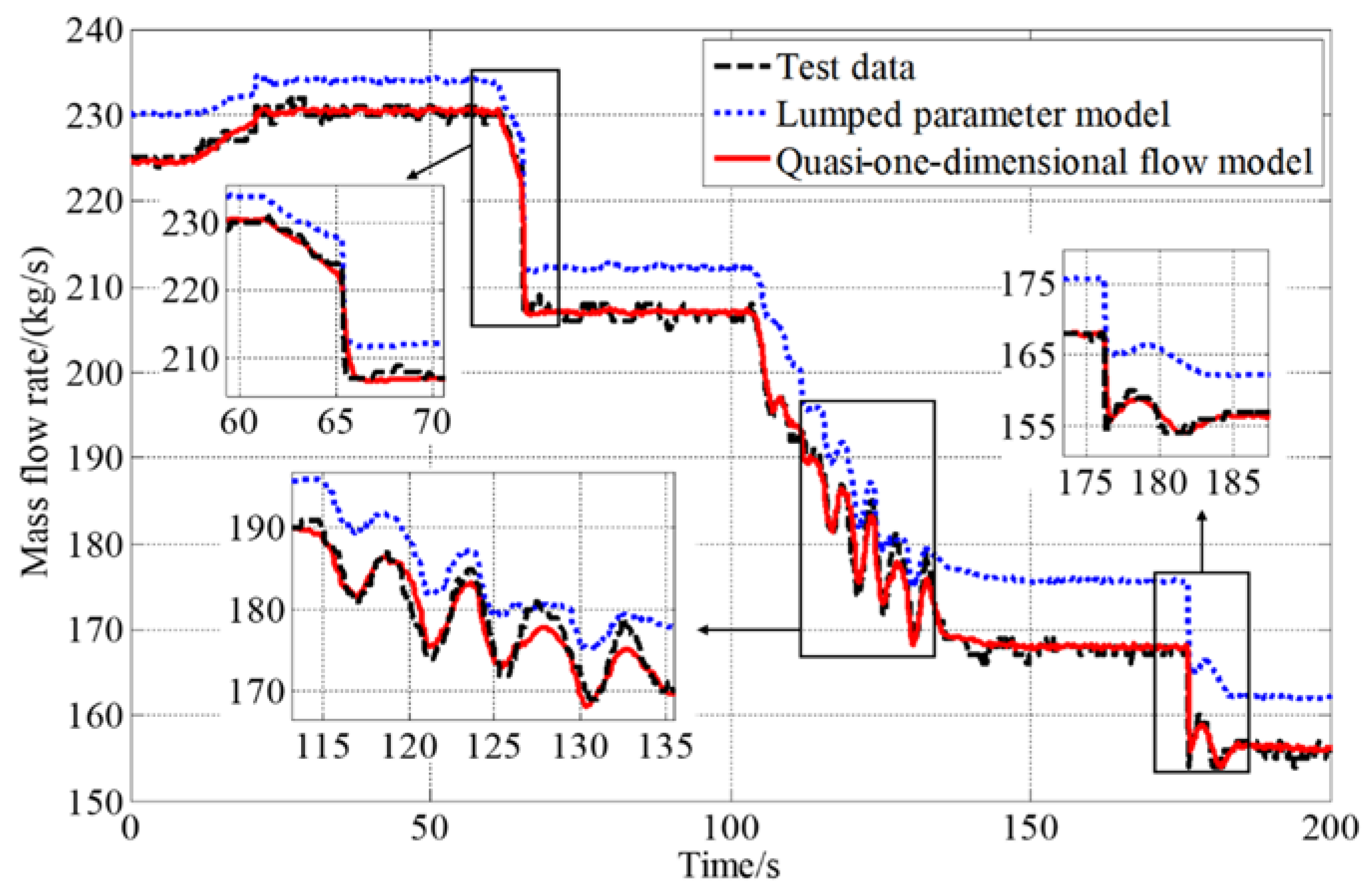
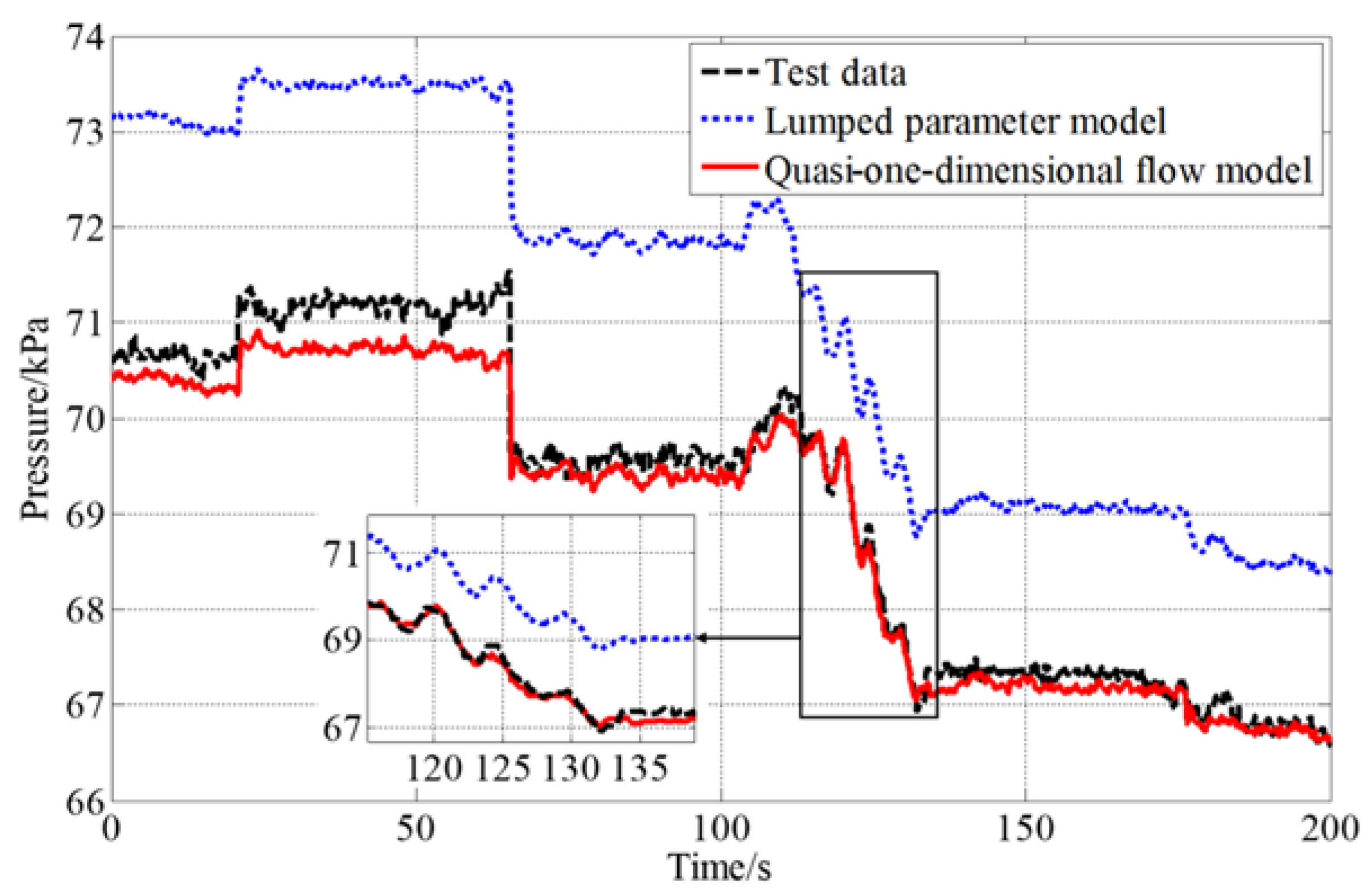
5.1. Difference between Quasi-One-Dimensional Flow Model and Lumped Parameter Model

According to Ref. [8], an ASTF model based on the multi-volume modeling method was established. This model is essentially a lumped parameter model. The control valve and flow deflector were used as throttling components to model the entire system as a combination of multiple volumes, in which the buffer chamber and the special-shaped pipe together formed a large volume, as shown in Figure 15. Compared with the lumped parameter model, the quasi-one-dimensional flow model takes into account factors such as friction and local losses (see Equation (4)), and the influence of these factors can be directly seen by the following simulation.

Boundary conditions:

• The pressure and temperature of air source 1 were respectively 95.291 kPa and 282 K;
• The pressure and temperature of air source 2 were respectively 147.053 kPa and 396 K;
• The flow at air outlet was 223.2 kg/s.

The opening of control valve 1 was set to 72.6%. The opening of control valve 2 was maintained at 30% for 0~5 s (called stage 1) and stepped to 40% in the 5th second. The cross-section signs of ASTF are shown in Figure 12.

In stage 1, the pressure and temperature distribution of ASTF are listed in

Table 1. Pressure at different sections.

Modeling Method	Pressure/kPa
	A	B	C	D	E	F	G	H	I
Lumped parameter	88.4	88.4	90	90	86.4	76.6	76.6	76.6	76.6
Quasi-one-dimensional	88.6	87.8	91	89.6	85.9	78.6	71.6	74.4	72.4

and

Table 2. Temperature at different sections.

Modeling Method	Temperature/K
	A	B	C	D	E	F	G	H	I
Lumped parameter	282.3	282.3	395.9	395.9	341.3	336.1	336.1	336.1	336.1
Quasi-one-dimensional	281.7	281.8	394.9	395.2	343	343.1	341	342.4	340.6

. In fact, the lumped parameter model takes the pipeline between two throttling components as a volume. Therefore, the pressure and temperature of each cross section cannot be distinguished, and it is difficult to reflect the pressure and temperature gradients caused by expansion, bends, friction, and local obstacles. Conversely, the quasi-one-dimensional flow model can overcome these limitations and calculate the airflow parameters of the cross section where the real sensor is located. This lays the foundation for using sensor data to optimize the system-level model.

Select the equal-diameter straight pipeline at the outlet of ASTF and divide it into 91 nodes along the axial direction, as shown in Figure 12. When the opening of control valve 2 changed, the pressure and temperature of each node began to change with time. It can be seen from Figure 16 that the quasi-one-dimensional flow model can reflect the propagation process of the airflow. This means that ASTF has a time-delay characteristic, which provides a more realistic simulation environment for controller design and verification. However, for the lumped parameter model, the properties of the airflow are assumed to be instantaneously uniform in the pipeline, which cannot reflect the dynamic changes of the airflow parameters in space. When the pipeline is longer, it will cause a larger deviation. In addition, the flow characteristics of the airflow along the pipeline make the heat transfer process have spatial distribution characteristics, which can more accurately simulate the impact of the metal pipeline on the airflow energy.

5.2. Model Verification Based on Test Data

To verify the accuracy of the quasi-one-dimensional flow model, the data measured by the sensors during the operation of ASTF were selected for simulation. The boundary conditions were the pressure and temperature measured by the sensors located at air sources 1, 2 and the air outlet. The valve opening measured by the displacement sensor was used as the input of the control valve model. The initial state of the model was set according to the ASTF system state at the beginning of the test data. The parameters to be compared were the mass flow (measured by the flow tube at the outlet) and the mixer pressure. The locations of these sensors are shown in Figure 12. In addition, for comparative analysis, the above simulation conditions were also applied to the lumped parameter model established according to Ref. [8], and the simulations were carried out.

The boundary conditions and valve opening are shown in Figure 17.

The comparison result of the mass flow rate at the air outlet is shown in Figure 18. Compared with the lumped parameter model, the simulation result of the quasi-one-dimensional flow model is more consistent with the test data in the steady state and dynamic process. In fact, the quasi-one-dimensional flow model has pressure losses caused by friction and cross-sectional area changes, resulting in different pressure distributions in ASTF. This makes the pressure ratio of the throttling component different in the two models, causing a difference in mass flow. It is worth noting that when studying the lumped parameter model in the past, this error between simulation data and test data is usually attributed to the inaccuracy of the control valve characteristic. However, the simulation result here reveals the defects of the lumped parameter model. Compared with the test data, the mass flow error results of the quasi-one-dimensional flow model are shown in Figure 19. The steady-state relative error is less than 1.5%, and the dynamic relative error is less than 2.2%.

Figure 20 shows the pressure comparison result of the mixer. The pressure dynamics of the two models are basically consistent with the test data. Compared with the quasi-one-dimensional flow model, the pressure error of the lumped parameter model is larger, and the average pressure error is about 2 kPa, which is consistent with the simulation result of Ref. [8]. The pressure error results of the quasi-one-dimensional flow model are shown in Figure 21. In 20–65 s, the mass flow reaches the maximum, and the pressure error increases. At 65 s, the rapid action of the control valve causes a large dynamic pressure change, and the relative pressure error is less than 1.4%. In 65–200 s, the mass flow is relatively low, and the relative pressure error is less than 0.6%.

6. Conclusions

In this study, a generic quasi-one-dimensional flow modeling method was used to establish a numerical simulation model of ASTF. Thereafter, the simulation and verification of the model were carried out. The main conclusions are summarized as follows.

(1)

Compared with the lumped parameter model, the quasi-one-dimensional flow model can simulate spatial effect and time delay of the airflow.

(2)

The simulation results of the quasi-one-dimensional flow model are basically consistent with the test data. The relative errors of mass flow and pressure are less than 2.2% and 1.4%, respectively, further verifying the correctness of the proposed modeling method.

(3)

With the generic modeling method, the system-level model still has the form of a staggered grid, and the properties of quasi-one-dimensional flow, such as spatial effect and time delay can be easily addressed during the modeling process.

In the future, the friction factor and the minor loss coefficient will be calibrated through the test data to further improve the model accuracy.

References

- Wang, X.; Zhu, M.Y.; Zhang, S.; Dan, Z.H.; Pei, X.T. Technology Development of Foreign Altitude Simulation Test Facilities Control System. Gas Turb. Exp. Res. 2017, 30, 49–55. Available online: https://kns.cnki.net/kcms/detail/detail.aspx?FileName=RQWL201706011&DbName=CJFQ2017 (accessed on 15 April 2022). (In Chinese).
- Tian, J.H.; Dan, Z.H.; Zhang, S.; Wang, X. Environment Simulation Control Technology for Altitude Test Facility. Aerosp. Power 2021, 3, 64–68. Available online: https://kns.cnki.net/kcms/detail/detail.aspx?FileName=HKDL202103019&DbName=CJFQ2021 (accessed on 15 April 2022). (In Chinese).
- Schmidt, K.J.; Merten, R.; Menrath, M.; Braig, W. Adaption of the Stuttgart University Altitude Test Facility for BR700 Core Demonstrator Engine Tests. In Proceedings of the ASME International Gas Turbine & Aeroengine Congress & Exhibition: The American Society of Mechanical Engineers, Stockholm, Sweden, 2–5 June 1998. [Google Scholar] [CrossRef] [Green Version]
- Montgomery, P.A.; Burdette, R.; Krupp, B. A Real-Time Turbine Engine Facility Model and Simulation for Test Operations Modernization and Integration. In Proceedings of the ASME Turbo Expo 2000: Power for Land, Sea, and Air, Munich, Germany, 8–11 May 2000. [Google Scholar] [CrossRef]
- Montgomery, P.A.; Burdette, R.; Wilhite, L.; Salita, S. Modernization of a Turbine Engine Test Facility Utilizing a Real-Time Facility Model and Simulation. In Proceedings of the ASME Turbo Expo 2001: Power for Land, Sea, and Air, New Orleans, LA, USA, 4–7 June 2001. [Google Scholar] [CrossRef]
- Sheeley, J.M.; Sells, D.A.; Bates, L.B. Experiences with Coupling Facility Control Systems with Control Volume Facility Models. In Proceedings of the 42nd AIAA Aerospace Sciences Meeting and Exhibit, Reno, NE, USA, 5–8 January 2004. [Google Scholar] [CrossRef]
- Pei, X.T.; Zhang, S.; Dan, Z.H.; Zhu, M.Y.; Qian, Q.M.; Wang, X. Study on Digital Modeling and Simulation of Altitude Test Facility Flight Environment Simulation System. J. Propul. Technol. 2019, 40, 1144–1152. (In Chinese) [Google Scholar] [CrossRef]
- Zhu, M.Y.; Wang, X.; Pei, X.T.; Zhang, S.; Dan, Z.H.; Miao, K.Q.; Liu, J.S.; Jiang, Z. Multi-Volume Fluid-Solid Heat Transfer Modeling for Flight Environment Simulation System. J. Propul. Technol. 2020, 41, 2848–2859. (In Chinese) [Google Scholar] [CrossRef]
- Boylston, B.M. Quasi-One-Dimensional Flow for Use in Real-Time Facility Simulations. Master’s Thesis, University of Tennessee, Knoxville, TN, USA, 2011. Available online: https://trace.tennessee.edu/utk_gradthes/1058 (accessed on 9 February 2022).
- Xu, Y.H. Research on Real-time Simulation Model and Algorithm for Incompressible Fluid Network Based on One-dimension Flow. Master’s Thesis, Harbin Engineering University, Harbin, China, 2009. (In Chinese). [Google Scholar] [CrossRef]
- Sun, K.; Liu, G.W.; Ma, C.T.; Niu, J.J. Calculation Model of Tube System and Value Based on 1D Network Model. J. Eng. Therm. 2017, 38, 1889–1895. Available online: https://kns.cnki.net/kcms/detail/detail.aspx?FileName=GCRB201709014&DbName=CJFQ2017 (accessed on 15 April 2022). (In Chinese).
- Tao, Z.; Hou, S.P.; Han, S.J.; Ding, S.T.; Xu, G.Q.; Wu, H.W. Study on Application of Fluid Network into the Design of Air System in Engine. J. Aerosp. Power 2009, 24, 1–6. (In Chinese) [Google Scholar] [CrossRef]
- Pei, X.T.; Liu, J.S.; Wang, X.; Zhu, M.Y.; Zhang, L.Y.; Dan, Z.H. Quasi-one-dimensional Flow Modeling for Flight Environment Simulation System of Altitude Ground Test Facilities. Processes 2022, 10, 377. (In Chinese) [Google Scholar] [CrossRef]
- Rennie, R.M.; Sutcliffe, P.; Vorobiev, A.; Cain, A.B. Mathematical Modeling of Wind-Speed Transients in Wind Tunnels. In Proceedings of the 51st AIAA Aerospace Sciences Meeting Including the New Horizons Forum and Aerospace Exposition, Grapevine, TX, USA, 7–10 January 2013. [Google Scholar] [CrossRef]
- Liu, K.; Cheng, M.S.; Zhang, Y.L. Dynamic Model of Priming Processes of Cryogenic Propellant Feed Lines. J. Natl. Univ. Def. Technol. 2003, 25, 1–5. (In Chinese) [Google Scholar] [CrossRef]
- Cheng, M.S.; Liu, K.; Zhang, Y.L. Numerical Analysis of Pre-cooling and Priming Transients in Cryogenic Propellant Feed Systems. J. Propul. Technol. 2000, 21, 38–41. (In Chinese) [Google Scholar] [CrossRef]
- Pan, J.S. Fundamentals of Gasdynamics; National Defense Industry Press: Beijing, China, 1989; pp. 40–63. (In Chinese) [Google Scholar]
- Çengel, Y.A.; Boles, M.A. Thermodynamics: An Engineering Approach, 5th ed.; McGraw-Hill: New York, NY, USA, 2006; pp. 219–232. [Google Scholar]
- Chen, Y.; Gao, F.; Zhang, Z.P.; Cai, G.B. Finite Volume Model for Quasi one-dimensional Compressible Transient Pipe Flow (I) Finite Volume Model of Flow Field. J. Aerosp. Power 2008, 23, 311–316. (In Chinese) [Google Scholar] [CrossRef]
- Zhu, M.Y.; Wang, X. An Integral Type µ Synthesis Method for Temperature and Pressure Control of Flight Environment Simulation Volume. In Proceedings of the ASME turbo Expo 2017: Turbomachinery Technical Conference and Exposition, Charlotte, NC, USA, 26–30 June 2017. (In Chinese). [Google Scholar] [CrossRef]
- Sutcliffe, P.; Vorobiev, A.; Rennie, R.M.; Cain, A.B. Control of Wind Tunnel Test Temperature Using a Mathematical Model. In Proceedings of the AIAA Ground Testing Conference, San Diego, CA, USA, 24–27 June 2013. [Google Scholar] [CrossRef]
- Çengel, Y.A. Heat Transfer: A Practical Approach; McGraw-Hill: New York, NY, USA, 2010; pp. 11–25. [Google Scholar]
- De Giorgi, M.G.; Fontanarosa, D. A Novel Quasi-one-dimensional Model for Performance Estimation of a Vaporizing Liquid Microthruster. Aerosp. Sci. Technol. 2019, 84, 1020–1034. [Google Scholar] [CrossRef]
- Liu, K.; Zhang, Y.L. Finite Elements State-space Model for One-dimensional Compressible Fluid Flow. J. Propul. Technol. 1999, 20, 62–66. (In Chinese) [Google Scholar] [CrossRef]
- Wang, X.Y. Fundamentals of Aerodynamics; Northwestern Polytechnical University Press: Xi’an, China, 2006; pp. 94–101. (In Chinese) [Google Scholar]
- Wang, M.D. Research of Tank Pressurization System of Liquid Rocket Engine Test-bed. Master’s Thesis, Shanghai Jiao Tong University, Shanghai, China, 2009. Available online: https://kns.cnki.net/kcms/detail/detail.aspx?FileName=2010200382.nh&DbName=CMFD2011 (accessed on 15 April 2022). (In Chinese).
- Pei, X.T.; Zhu, M.Y.; Zhang, S.; Dan, Z.H.; Wang, X.; Wang, X. An Iterative Method of Empirical Formula for the Calculation of Special Valve Flow Characteristics. Gas Turb. Exp. Res. 2016, 29, 35–39. Available online: https://kns.cnki.net/kcms/detail/detail.aspx?FileName=RQWL201605009&DbName=CJFQ2016 (accessed on 9 February 2022). (In Chinese).
- Wang, Y.L.; Wang, X.; Zhu, M.Y.; Pei, X.T.; Zhang, S.; Dan, Z.H. Comparative Study on Modeling Methods of Special Control Valves in Altitude Simulation Test Facility. J. Propul. Technol. 2019, 40, 1895–1901. (In Chinese) [Google Scholar] [CrossRef]