Cornish–Fisher-Based Control Charts Inclusive of Skewness and Kurtosis Measures for Monitoring the Mean of a Process

Abstract

In this paper, we propose control limits for monitoring the mean of a process variable based on a first and second order Cornish–Fisher expansion, which limits are inclusive of its skewness and kurtosis measures, respectively. These are shown to have better in-control error performance than other limits that were similarly derived from this expansion with smoothing functions, both when these measures are assumed to be known and estimated from sample data. The range of measure specifications where the underlying Cornish–Fisher function is monotonic is derived. Operating characteristic curves for select cases demonstrate the associated out-of-control error performance. The Cornish–Fisher limits are applied to a real-life dataset in developing a control chart for monitoring the mean lifetime of car brake pads, wherein they are compared to other limit approximations.

1. Introduction

The classic Shewhart $\overline{X}$ control chart on the mean of a process specifies control limits as the in-control mean plus/minus a multiplier of the standard deviation of the distribution of the sample mean. The skewness and excess kurtosis are omitted from this specification, and assumed to vanish by the central limit theorem when determining the type 1 and 2 error rates of these limits. In the case where these measures deviate greatly from zero in the population distribution, however, convergence to the Gaussian distribution may not be reasonably assumed for small subgroup sizes. Indeed there are many examples of real world processes in healthcare, tool wear, and human performance that follow Gamma, lognormal, and other non-Gaussian distributions with a high degree of skewness and kurtosis, for which Shewhart $\overline{X}$ limits may be largely inaccurate for assumed error rates [1,2,3].

One method to handle such cases is to use a moment-based expansion of the sampling distribution of the mean that includes estimates of the population skewness or both skewness and kurtosis. In particular, a Cornish–Fisher (CF) expansion is one such method that may be used to approximate the corresponding quantile function that is inclusive of the skewness when truncated at the first order and of both skewness and kurtosis when truncated at the second order. Building on this, reference [4] utilized a first order CF expansion (CF-1) in specifying control limits that incorporated the skewness measure referred to as skewness correction (SC) limits, and reference [5] utilized a second order CF expansion (CF-2) in specifying limits that incorporated a kurtosis, but not skewness, measure referred to as Kurtosis Correction (KC) limits. While these showed improvement over Shewhart and other heuristic limits in select cases, they are specified with a smoothing function that increasingly negates the contribution of the estimated skewness and kurtosis measures to the approximated limits when these are increased in absolute value. This smoothing function gets around the inherent bounding of the skewness and kurtosis in the CF expansion, outside of which the approximated quantile function may not be monotonically increasing. These bounds are referred to as the domain of validity [6], and consist of one-dimensional range of skewness values for a CF-1 expansion and a two-dimensional range of skewness and kurtosis values for a CF-2 expansion. However, it was observed that the domain of validity of the skewness and kurtosis measure of both the CF-1 and CF-2 expansions are sufficiently quite wide to capture most practical applications of statistical process control. Indeed, a study by [7] found that the vast majority of real-world data sets that were studied had ranges of skewness and kurtosis values in the population distribution that would fall within the domain of validity of the CF-1 and CF-2 expansions when considering common subgroup sizes $n\ge 3$. Furthermore, the CF expansions will continue to exist outside the domain of validity, yet with likely diminished accuracy.

Other approaches to this problem include control charts that are based in other parametric approximations or in a non-parametric method. Weighted standard deviation (WSD) [8] and improved exponentially weighted moving average (IEWMA) [9] are two common parametric-based charts. The WSD method modifies Shewhart limits by having separate standard deviations for the LCL and the UCL where these are modified by the probability that the sample will be less than or greater than the mean respectively. It was demonstrated in [4] that the SC method based on Cornish–Fisher approximations outperformed the WSD method for every skewed distribution considered, for both known and estimated skewness. The IEWMA method selects a smoothing function and weights a priori to determine the effects of skewness on the control limits. Studies by [10,11] have shown that the IEWMA method overestimates the average run length (ARL) significantly when the mean and variance are estimated from data, and can be highly subjective to the assigned smoothing function and weights. Non-parametric control charts monitor a process median through order statistics or ranks of collected data, rather than directly monitoring the process mean. A sampling of such charts include [12] and a review of these may be found in [13]. Non-parametric charts by definition require no distributional assumption, yet likewise do not incorporate information about the skewness and kurtosis measures into the specification of the control limits. An example non-parametric chart that produces a Shewhart type control chart is the mean-rank chart proposed by [14]. The mean-rank chart utilizes the well-known Kruskal–Wallis nonparametric test [15] and converges to control limits set by the standard normal distribution as the sample size increases with the central limit theorem. Two other, closely related non-parametric Shewhart type control charts are the sign [16] and the signed-rank [17] control charts. Although all three non-parametric methods perform well for small shifts in the process variable, there is a cost in terms of sample size for accuracy.

In this paper, we present control limits for a $\overline{X}$ chart that are derived directly from the CF-1 and CF-2 expansions without smoothing functions, thereby fully incorporating estimates of the skewness and the skewness and excess kurtosis into the approximated control limits. These are referred to as CF-1 and CF-2 limits in this paper, and are an alternative to SC and KC limits that are also based on a Cornish–Fisher expansion. These limits will be numerically tested across a range of subgroup sizes and asymmetrical population distributions, wherein they will be compared in their ability to meet a target in-control average run length (ARL). This testing will be in both the case in which the skewness and kurtosis measures are assumed to be known, and in the case where these are estimated from data. Additionally, the out-of-control performance of the CF-2 chart will assessed for the cases considered. Following this, an $\overline{X}$ chart with the aforementioned limit approximation will be applied to a real-world data set for comparison purposes.

2. CF-1 Limits Inclusive of Skewness

It was shown by [18] that for a subgroup of size n, the random variable $\overline{X}$ at the pth quantile, ${\overline{X}}_p$, can be estimated by inverting an Edgeworth expansion through the jth order, yielding a standard normal quantile function, ${\Phi }^{-1}\left(p\right)$, as the argument to polynomial functions of higher order cumulants [19]. When truncating at the first order, the CF-1 expansion given by

$${\overline{X}}_p\approx \mu +\frac{\sigma }{\sqrt{n}}\left(Z_p+\left[\frac{Z_p^2-1}{6}\left(\frac{{\nu }_3}{\sqrt{n}}\right)\right]\right)$$

(1)

where

$$Z_p={\Phi }^{-1}\left(p\right)$$

is inclusive of the skewness (${\nu }_3$) measure. Letting $p=\alpha /2=0.0027/2$, as is common for process monitoring, it follows that

$$Z_{0.00135}=\pm 3,$$

(2)

whereupon substitution into Equation (1) yields the following CF-1 control limits

$$\begin{array}{ccc}\hfill UCL& =& \mu +\frac{\sigma }{\sqrt{n}}\left(3+\frac{4{\nu }_3}{3\sqrt{n}}\right)\hfill \\ \hfill LCL& =& \mu +\frac{\sigma }{\sqrt{n}}\left(-3+\frac{4{\nu }_3}{3\sqrt{n}}\right).\hfill \end{array}$$

(3)

As a matter of comparison, the SC limits of [4] are given by

$$\begin{array}{ccc}\hfill UCL& =& \mu +\frac{\sigma }{\sqrt{n}}\left(3+\frac{4{\nu }_3}{3\sqrt{n}}\left(\frac{n}{n+0.2{\nu }_3^2}\right)\right)\hfill \\ \hfill LCL& =& \mu +\frac{\sigma }{\sqrt{n}}\left(-3+\frac{4{\nu }_3}{3\sqrt{n}}\left(\frac{n}{n+0.2{\nu }_3^2}\right)\right).\hfill \end{array}$$

(4)

Note that the contribution of the skewness measure to the specification of the SC control limits vanishes as such is increased in absolute value, limiting these to Gaussian/Shewhart control limits.

The domain of validity for the CF-1 expansion of Equation (1) is that where the first derivative is non-negative, given by

$$\begin{array}{ccc}\hfill \frac{d{\overline{X}}_p}{d{Z}_p}& =& Z_p\left[\frac{{\nu }_3}{3\sqrt{n}}\right]+1\ge 0,\hfill \end{array}$$

from whence

$$\begin{array}{c}\hfill \frac{{\nu }_3}{\sqrt{n}}\ge \frac{-3}{Z_p}.\end{array}$$

Substituting Equation (2) yields the following domain of validity

$$\begin{array}{c}\hfill -1\le \frac{{\nu }_3}{\sqrt{n}}\le 1.\end{array}$$

(5)

for the skewness measure encompassed within the $\alpha =0.0027$ control limits.

3. CF-2 Limits Inclusive of Skewness and Kurtosis

When truncating at the second order, the CF-2 expansion given by

$${\overline{X}}_p\approx \mu +\frac{\sigma }{\sqrt{n}}\left(Z_p+\left[\frac{Z_p^2-1}{6}\left(\frac{{\nu }_3}{\sqrt{n}}\right)\right]+\left[\frac{Z_p^3-3Z_p}{24}\left(\frac{{\nu }_4}{n}\right)-\frac{2Z_p^3-5Z_p}{36}\left(\frac{{\nu }_3^2}{n}\right)\right]\right)$$

(6)

where

$$Z_p={\Phi }^{-1}\left(p\right)$$

is inclusive of both the skewness (${\nu }_3$) and excess kurtosis (${\nu }_4$) measures. Letting $p=\alpha /2=0.0027/2$, the CF-2 limits follow from Equation (6) as

$$\begin{array}{ccc}\hfill UCL& =& \mu +\frac{\sigma }{\sqrt{n}}\left(3+\frac{4}{3}\left(\frac{{\nu }_3}{\sqrt{n}}\right)-\frac{13}{12}\left(\frac{{\nu }_3^2}{n}\right)+\frac{3}{4}\left(\frac{{\nu }_4}{n}\right)\right)\hfill \\ \hfill LCL& =& \mu +\frac{\sigma }{\sqrt{n}}\left(-3+\frac{4}{3}\left(\frac{{\nu }_3}{\sqrt{n}}\right)+\frac{13}{12}\left(\frac{{\nu }_3^2}{n}\right)-\frac{3}{4}\left(\frac{{\nu }_4}{n}\right)\right)\hfill \end{array}$$

(7)

As a matter of comparison, the KC limits of [5] are given by

$$\begin{array}{ccc}\hfill UCL& =& \mu +\frac{\sigma }{\sqrt{n}}\left(3+\frac{{\nu }_4}{n+0.33{\nu }_4}\right)\hfill \\ \hfill LCL& =& \mu +\frac{\sigma }{\sqrt{n}}\left(-3-\frac{{\nu }_4}{n+0.33{\nu }_4}\right).\hfill \end{array}$$

(8)

Note that in the KC limits of (8), skewness is omitted and the effect of kurtosis limits to one when increased in absolute value.

The domain of validity for the CF-2 expansion of (6) is found as

$$\frac{d{X}_p}{d{Z}_p}=Z_p^2\left[\frac{{\nu }_4}{8n}-\frac{{\nu }_3^2}{6n}\right]+Z_p\left[\frac{{\nu }_3}{3\sqrt{n}}\right]+\frac{5{\nu }_3^2}{36n}-\frac{{\nu }_4}{8n}+1\ge 0$$

(9)

which will hold if the corresponding discriminant $\Delta$ is negative. Hence, it follows that

$$\begin{array}{ccc}\hfill \Delta & =& \frac{{\nu }_3^2}{9n}-4\left[\frac{5{\nu }_3^2}{36n}-\frac{{\nu }_4}{8n}+1\right]\left[\frac{{\nu }_4}{8n}-\frac{{\nu }_3^2}{6n}\right]\le 0,\hfill \end{array}$$

(10)

for all quantiles p, from whence the two-dimensional region of validity for the skewness and kurtosis measures of the distribution of the mean is depicted in Figure 1, with maximal values given by $-2.489\le \frac{{\nu }_3}{\sqrt{n}}\le 2.489$ and $0\le \frac{{\nu }_4}{n}\le 11.549$.

4. Numerical Analysis

The accuracy of the Cornish–Fisher limits were tested in terms of their ability to meet the specified type-1 error rate $\alpha$, which is expressed for convenience as the in-control average run length (ARL) given by

$$ARL=1/\alpha .$$

Since the population distribution is assumed to be asymmetric, these will be measured separately for the approximated upper and lower limits, for which the specified type-1 error rate above the UCL (ARL↑) and below the LCL (ARL↓) will be set to the commonly assumed value of $\alpha /2=0.0027/2=0.00135$, and hence the exact $ARLs$ given by

$$ARL\uparrow =ARL\downarrow =740.74.$$

(11)

The process variable in this numerical study is assumed to follow a $Gamma(\gamma ,1/\lambda )$ probability distribution, yet it should be noted that the control limits are specified through the moments of the random variable and not the distribution of such. The $Gamma$ distribution was selected for this study due to its ability to both model a broad range of asymmetric shapes and obtain a closed form expression for the distribution of the subgroup mean, i.e., $\overline{X}$∼$Gamma(n\gamma ,1/n\lambda )$, from whence exact ARL values for the approximated limits may be obtained. It follows thus that the accuracy of the approximated limits may be compared to the exact values of Equation (11) when the corresponding measures of the population mean, variance, skewness, and kurtosis measures are either assumed to be known or estimated from sampled data, evaluating thus both theoretical and practical accuracy.

4.1. Known Skewness and Kurtosis Measures

The theoretical accuracy of the CF-1 and CF-2 limits of Equations (3) and (7) for subgroup sizes of $n=5,10,15$ were compared to exact, Gaussian/Shewhart, and the SC and KC limits of Equations (7) and (8) for a $Gamma(\gamma ,1/\lambda )$ distributed process variable with $1/\lambda =3$ and $\gamma =1,2,4$, as depicted in Figure 2.

As shown in Figure 2, the $Gamma(\gamma ,1/\lambda )$ distribution can assume a wide array of possible skew and kurtosis values present in datasets. Note that a $Gamma(\gamma =1,1/\lambda =3)$ distributed process variable is an exponential distribution, and the distribution of the mean of both Chi-square and Weibull distributions are specialized cases of the $Gamma(n\gamma ,1/n\lambda )$ distribution. In addition to the control limits generated from a Cornish–Fisher expansion, those generated by the weighted standard deviation (WSD) method were likewise considered in this analysis.

The known summary measures of a $Gamma(n\gamma ,1/n\lambda )$ distribution are given by

$$\begin{array}{ccc}\hfill \mu & =& \frac{\gamma }{\lambda }\hfill \\ \hfill \frac{\sigma }{\sqrt{n}}& =& \frac{\sqrt{\gamma }}{\sqrt{n}\lambda }\hfill \\ \hfill \frac{{\nu }_3}{\sqrt{n}}& =& \frac{2}{\sqrt{n\gamma }}\hfill \\ \hfill \frac{{\nu }_4}{n}& =& \frac{6}{n\gamma }.\hfill \end{array}$$

(12)

Note that the skewness and kurtosis measures in the equations of (12) all fall within the domain of validity for both the CF-1 and CF-2 approximations as per Equations (5) and (10) for the specifications of n, $\gamma$, and $\lambda$ considered in this study. The corresponding control limits and in-control Average Run Lengths are given in

Table 1. Upper and lower control limits and in-control average run lengths for an $\overline{X}$-chart on a $Gamma(\gamma ,\frac{1}{\lambda })$ distributed process with subgroups of size n and desired type-1 error of $\alpha =0.0027$.

	Gamma (1,3) = Exponential(3)
	n = 5				n = 10				n = 15
	ARL↓	LCL	UCL	ARL↑	ARL↓	LCL	UCL	ARL↑	ARL↓	LCL	UCL	ARL↑
Exact	740.74	0.48	8.64	740.74	740.74	0.93	6.65	740.74	740.74	1.20	5.86	740.74
Gaussian	∞	(·)	7.03	107.41	4.56 × 10${}^9$	0.15	5.85	148.85	3.53 × 10${}^5$	0.68	5.23	179.09
WSD	-	-	7.50	187.62	-	-	6.08	234.80	9.71 × 10${}^6$	0.52	5.48	269.40
SC	2724.80	0.35	8.40	556.79	646.24	0.89	6.59	946.97	679.81	1.18	5.83	821.70
KC	333,333	0.128	8.18	422.30	14,705.88	0.63	6.32	377.22	7575.76	0.95	5.60	363.90
CF1	326.58	0.58	8.62	730.99	593.82	0.95	6.65	730.46	662.25	1.21	5.86	731.53
CF2	460.83	0.53	8.67	772.80	670.24	0.94	6.66	754.24	749.06	1.20	5.87	749.06
	Gamma (2,3)
	n = 5				n = 10				n = 15
	ARL↓	LCL	UCL	ARL↑	ARL↓	LCL	UCL	ARL↑	ARL↓	LCL	UCL	ARL↑
Exact	740.74	1.85	13.31	740.74	740.74	2.76	10.83	740.74	740.74	3.24	9.82	740.74
Gaussian	4.56 × 10${}^9$	0.31	11.69	148.85	5.20 × 10${}^4$	1.98	10.03	203.11	1.25 × 10${}^4$	2.71	9.29	240.16
WSD	-	-	12.18	237.76	3.33 × 10${}^5$	1.74	10.27	296.03	3.45 × 10${}^4$	2.56	9.45	336.47
SC	946.97	1.79	13.17	646.83	783.70	2.74	10.79	696.38	732.06	3.24	9.81	712.76
KC	14,705.88	1.26	12.64	377.22	5405.41	2.34	10.39	361.14	3703.70	2.92	9.49	366.03
CF1	593.82	1.91	13.29	730.46	689.66	2.775	10.82	733.14	711.74	3.25	9.82	734.21
CF2	670.24	1.88	13.32	754.72	722.02	2.76	10.84	746.83	732.06	3.24	9.83	744.05
	Gamma (4,3)
	n = 5				n = 10				n = 15
	ARL↓	LCL	UCL	ARL↑	ARL↓	LCL	UCL	ARL↑	ARL↓	LCL	UCL	ARL↑
Exact	740.74	5.52	21.66	740.74	740.74	7.10	18.50	740.74	740.74	7.88	17.18	740.74
Gaussian	5.20 × 10${}^4$	3.95	20.05	203.11	6765.87	6.31	17.69	268.31	3755.31	7.35	16.65	309.84
WSD	3.33 × 10${}^5$	3.46	20.52	292.74	1.50 × 10${}^4$	6.06	17.93	358.68	6578.95	7.19	16.80	397.61
SC	783.70	5.49	21.59	696.38	735.29	7.10	18.48	720.46	744.05	7.88	17.17	728.33
KC	5405.41	4.68	20.79	361.14	2976.19	6.58	17.96	374.81	2298.85	7.50	16.80	393.24
CF1	689.66	5.55	21.65	733.14	720.98	7.11	18.49	735.29	729.39	7.89	17.18	736.92
CF2	722.02	5.53	21.67	746.83	735.29	7.10	18.50	742.94	738.01	7.88	17.19	742.39

$(·$) = observation outside domain of definition; $ARL\downarrow =1/Pr\left\{\overline{X}<LCL\right\}$ for $\overline{X}$∼$Gamma(n\gamma ,1/n\lambda )$; $ARL\uparrow =1/Pr\left\{\overline{X}>UCL\right\}$ for $\overline{X}$∼$Gamma(n\gamma ,1/n\lambda )$.

.

In comparing performance, most all approximated limits outperform Gaussian/Shewhart limits, yet it is further evident that the CF-1 and CF-2 approximations outperform all other methods across specification of the shape parameter $\gamma$ and subgroups sizes n. Of particular interest, they outperform the SC and KC limits which were derived from the CF-1 and CF-2 expansions with the addition of the smoothing function. Specific to the SC limits, the CF-1 limits, which also only incorporates skewness, has similar performance for cases with limited asymmetry in the population distribution or large subgroup sizes, yet largely outperforms the SC limits at higher degrees of asymmetry and small subgroup sizes. The CF-2 limits, which additionally incorporates kurtosis, outperform SC and CF-1 limits in all instances. The KC limits have generally poor performance due to the assumption of these that the skewness is equal to zero.

From Table 1, it is observed that the in-control ARL performance of the lower control limit (LCL) for all approximate limits demonstrate a high degree of inaccuracy, e.g., $n=5$ from a $Gamma(1,3)$ distribution. Since the skewness is positive, it is noted that the derivative of the distribution of the mean in the lower tail increases greatly for small subgroup sizes and, hence, any deviation from the exact specification of the LCL will have a large deviation from the target type 1 error. Specific to the CF-1 and CF-2 limits, the magnitude of the associated skewness and kurtosis push towards the boundaries of the domain of validity of the Cornish–Fisher expansion, causing further inaccuracy, yet it is noted that this continues to be more accurate than the other limits.

The type-2 error performance of the approximate distributions was assessed by varying the values of the parameters $\gamma$ and $1/\lambda$ and generating the corresponding operating characteristic (OC) curves in Figure 3 and Figure 4. The OC curves only display the CF-2 approximations since the CF-1 approximation is very similar and would be difficult to determine the distinction between each graphically. The similarity between CF-1 and CF-2 approximations is demonstrated in a specific case presented in

Table 2. In- and out-of-control ARLs for a $Gamma(\gamma =2,\frac{1}{\lambda }=3)$ distributed process with subgroups of size $n=5$.

	$1/\mathit{\lambda }$	Exact	Gaussian	CF-1	CF-2
ARL↓	1	2.24	8.13 × 10${}^4$	2.06	2.16
	2	49.48	8.13 × 10${}^4$	41.27	45.56
	3	740.74	4.56 × 10${}^9$	593.82	670.24
ARL↑	3	740.74	148.58	520.02	754.72
	4	31.69	12.00	31.42	32.06
	5	6.87	3.70	6.79	6.87
$ARL\downarrow =1/Pr\left\{\overline{X}<LCL\right\}$ for $\overline{X}\sim Gamma(n\gamma ,1/n\lambda )$
$ARL\uparrow =1/Pr\left\{\overline{X}>UCL\right\}$ for $\overline{X}\sim Gamma(n\gamma ,1/n\lambda )$

.

Note that when shifting the scale parameter, both the mean and variance of $\overline{X}$ vary, yet the skewness and kurtosis remain constant, whereas when shifting the shape parameter, all measures of $\overline{X}$ vary.

Based on Figure 3 and Figure 4, the Gaussian approximation is not accurate in detecting shifts for both the LCL and UCL. CF-1 and CF-2 approximations predict out-of-control performance for all shifting shape and scale parameters almost the same as the exact $Gamma(\gamma ,1/\lambda )$ distribution’s control limits. Consider the specific case of a $Gamma(2,3)$ distribution with subgroups of size $n=5$, whose in- and out-of-control ARL performance is given in Table 2. In all cases given in Table 2, the CF-1 and CF-2 approximations achieve marked improvement over the normal approximation for type-2 errors. Of note, the Gaussian approximation generally displays loss of power as the shift increases in both directions. The Cornish–Fisher approximation only has a minimal loss of power on the order of a few percent relative error when compared with the exact ARL. There is also very minor differences between the CF-1 and CF-2 approximation except at the in-control ARL where the CF-2 approximation is more accurate. This reflects the previous results for the type-1 errors discussed in Table 1.

4.2. Estimated Skewness and Kurtosis Measures

As the skewness and kurtosis measures of a distribution are generally not known, the practical accuracy of the CF-1 and CF-2 limits are assessed in the same instances considered previously when the measures of the distribution of the mean are estimated from $n=m\ast n$ sampled data points as

$$\begin{array}{ccc}\hfill \widehat{\mu }& =& \overline{\overline{X}}=\frac{{\sum }_{i=1}^N{X}_i}{N}\hfill \\ \hfill \frac{\widehat{\sigma }}{\sqrt{n}}& =& \frac{1}{\sqrt{n}}\left(\frac{\sqrt{{\sum }_{i=1}^N{(X_i-\overline{\overline{X}})}^2}}{\sqrt{N-1}}\right)\hfill \\ \hfill \frac{\widehat{{\nu }_3}}{\sqrt{n}}& =& \frac{1}{\sqrt{n}}\left(\frac{\sqrt{N}{\sum }_{i=1}^N{(X_i-\overline{\overline{X}})}^3}{{\left({\sum }_{i=1}^N{(X_i-\overline{\overline{X}})}^2\right)}^{3/2}}\right)\hfill \\ \hfill \frac{\widehat{{\nu }_4}}{n}& =& \frac{1}{n}\left(\frac{N{\sum }_{i=1}^N{(X_i-\overline{\overline{X}})}^4}{{\left({\sum }_{i=1}^N{(X_i-\overline{\overline{X}})}^2\right)}^2}-3\right),\hfill \end{array}$$

(13)

Towards this end, a simulation study was conducted in which the ARL of Shewhart/Gaussian, SC, CF-1, and CF-2 limits were evaluated for each of $J=1000$ replications within each combination of the shape parameter $\gamma =1,2,3$, subgroup sizes $n=5,10,15$, and pre-sampled subgroups $m=100,1000,$ 10,000, whereupon the median (Med) and inner-quartile range (IQR) of these are reported for the LCL in

Table 3. In-control ARLs for the LCL of an $\overline{X}$-chart on a $Gamma(\gamma ,1/\lambda )$ distributed process.

		Gamma (1,3) = Exponential (3)
		n = 5			n = 10			n =15
	m =	100	1000	10,000	100	1000	10,000	100	1000	10,000
Exact		740.74	740.74	740.74	740.74	740.74	740.74	740.74	740.74	740.74
Gaussian	Known Sim(Med) Sim(IQR)	· · ·	· · ·	· · ·	4.56 × 105 · ·	4.56 × 105 · ·	4.56 × 105 · ·	3.53 × 105 (2.44 × 105) (4.24 × 105)	3.53 × 105 (3.29 × 105) (6.90 × 105)	3.53 × 105 (3.51 × 105) (1.95 × 105)
SC	Known Sim(Med) Sim(IQR)	2724.80 (16,042.05) (528,697.80)	2724.80 (3726.37) (5890.05)	2724.80 (2907.68) (1403.73)	946.97 (1625.76) (3458.58)	946.97 (1049.20) (708.76)	946.97 (956.43) (224.51)	821.69 (1179.06) (2574.73)	821.69 (856.85) (538.85)	821.69 (828.91) (168.45)
CF1	Known Sim(Med) Sim(IQR)	326.58 (1967.59) (15,430.76)	326.58 (437.12) (686.78)	326.58 (341.57) (181.22)	593.82 (1145.34) (2564.59)	593.82 (678.78) (515.40)	593.82 (606.50) (158.59)	662.25 (899.93) (1862.49)	662.25 (717.41) (408.27)	662.25 (668.68) (138.78)
CF2	Known Sim(Med) Sim(IQR)	460.83 (333.84) (867.29)	460.83 (358.80) (287.72)	460.83 (419.56) (164.86)	670.24 (639.42) (1074.77)	670.24 (620.09) (311.65)	670.24 (657.01) (113.83)	749.06 (703.01) (1285.62)	749.06 (679.43) (353.41)	749.06 (699.11) (124.33)
		Gamma (2,3)
		n = 5			n = 10			n = 15
	m =	100	1000	10,000	100	1000	10,000	100	1000	10,000
Exact		740.74	740.74	740.74	740.74	740.74	740.74	740.74	740.74	740.74
Gaussian	Known Sim(Med) Sim(IQR)	4.56 × 109 · ·	4.56 × 109 · ·	4.56 × 109 · ·	5.20 × 104 (3.78 × 104) (3.20 × 105)	5.20 × 104 (5.00 × 104) (6.15 × 104)	5.20 × 104 (5.29 × 104) (1.81 × 104)	1.25 × 104 (1.02 × 104) (3.26 × 104)	1.25 × 104 (1.23 × 104) (1.24 × 104)	1.25 × 104 (1.27 × 104) (1092.90)
SC	Known Sim(Med) Sim(IQR)	946.97 (1468.95) (3042.21)	946.97 (1027.32) (695.96)	946.97 (950.96) (202.08)	783.70 (954.67) (1881.77)	783.70 (802.81) (404.00)	783.70 (786.45) (136.07)	758.15 (844.09) (1802.91)	758.15 (788.49) (438.33)	758.15 (757.03) (147.69)
CF1	Known Sim(Med) Sim(IQR)	593.82 (1007.22) (2222.62)	593.82 (671.91) (501.45)	593.82 (607.43) (157.25)	689.66 (876.56) (1860.54)	689.66 (710.90) (393.75)	689.66 (692.48) (122.72)	711.74 (828.37) (1851.38)	711.74 (719.21) (402.47)	711.74 (717.05) (131.09)
CF2	Known Sim(Med) Sim(IQR)	670.24 (540.62) (921.75)	670.24 (627.39) (327.84)	670.24 (654.38) (117.87)	722.02 (703.10) (1044.93)	722.02 (717.77) (332.00)	722.02 (720.22) (119.05)	732.06 (739.27) (1560.88)	732.06 (710.32) (383.10)	732.06 (734.96) (128.60)
		Gamma (4,3)
		n = 5			n = 10			n = 15
	m =	100	1000	10,000	100	1000	10,000	100	1000	10,000
Exact		740.74	740.74	740.74	740.74	740.74	740.74	740.74	740.74	740.74
Gaussian	Known Sim(Med) Sim(IQR)	5.20 × 104 (3.80 × 104) (2.15 × 105)	5.20 × 104 (4.98 × 104) (5.08 × 104)	5.20 × 104 (5.13 × 104) (1.58 × 104)	6765.87 (6776.40) (2.01 × 104)	6765.87 (6859.42) (4749.77)	6765.87 (6796.99) (1580.69)	3755.31 (3490.03) (1.13 × 10${}^5$)	3755.31 (3787.28) (3102.52)	3755.31 (3777.15) (901.67)
SC	Known Sim(Med) Sim(IQR)	783.70 (999.26) (1763.86)	783.70 (814.33) (418.17)	783.70 (795.62) (124.59)	749.63 (820.69) (1373.07)	749.63 (754.47) (363.18)	749.63 (751.03) (125.95)	744.05 (795.79) (1867.23)	744.05 (779.79) (429.59)	744.05 (736.71) (130.16)
CF1	Known Sim(Med) Sim(IQR)	689.66 (836.41) (1514.37)	689.66 (735.83) (396.29)	689.66 (690.93) (115.72)	720.98 (810.86) (1305.64)	720.98 (721.73) (389.33)	720.98 (729.00) (120.37)	729.39 (898.95) (1884.96)	729.39 (732.59) (414.86)	729.39 (720.67) (123.55)
CF2	Known Sim(Med) Sim(IQR)	722.02 (668.54) (875.65)	722.02 (721.95) (326.34)	722.02 (716.26) (104.11)	735.29 (772.98) (1219.99)	735.29 (724.90) (339.82)	735.29 (734.46) (105.75)	738.01 (721.21) (1645.47)	738.01 (710.36) (385.45)	738.01 (736.69) (133.52)

· Observation infinite or undefined; n = subgroup size, m = number of pre-samples from a $Gamma(\gamma ,1/\lambda )$ distribution; Exact ARL = 1/0.00135 = 740.74, calculated ARL = $1/Pr(\overline{X}<LCL)$ for $\overline{X}\sim Gamma(\gamma n,1/n\lambda )$; simulated results based on J = 1000 replications, Med = median, IQR = inner quartile range.

and UCL in

Table 4. In-control ARLs for the UCL of an $\overline{X}$-chart on a $Gamma(\gamma ,1/\lambda )$ distributed process.

		Gamma (1,3) = Exponential(3)
		n = 5			n = 10			n = 15
	m =	100	1000	10,000	100	1000	10,000	100	1000	10,000
Exact		740.74	740.74	740.74	740.74	740.74	740.74	740.74	740.74	740.74
Gaussian	Known Sim(Med) Sim(IQR)	107.41 (93.8) (89.33)	107.41 (103.72) (45.7)	107.41 (107.2) (13.05)	148.85 (131.49) (243.43)	148.85 (148.13) (83.48)	148.85 (147.73) (24.57)	179.09 (166.51) (336.02)	179.09 (174.83) (144.55)	179.09 (177.68) (33.91)
SC	Known Sim(Med) Sim(IQR)	556.79 (427.45) (941.62)	556.79 (544.22) (355.33)	556.79 (551.57) (109.13)	520.29 (368.39) (901.68)	520.29 (401.2) (371.98)	520.29 (523.16) (52.63)	562.75 (413.22) (1296.71)	562.75 (527.98) (441.37)	562.75 (566.73) (56.13)
CF1	Known Sim(Med) Sim(IQR)	730.99 (363.50) (1062.04)	730.99 (669.69) (451.69)	730.99 (724.90) (176.60)	730.46 (448.43) (1395.73)	730.46 (693.96) (516.92)	730.46 (723.59) (166.14)	731.53 (528.26) (1713.78)	731.53 (706.96) (511.33)	731.53 (727.27) (172.94)
CF2	Known Sim(Med) Sim(IQR)	772.80 (363.50) (999.44)	772.80 (669.79) (556.76)	772.80 (755.00) (245.50)	754.24 (442.48) (1144.96)	754.24 (664.23) (498.79)	754.24 (730.19) (177.53)	749.06 (485.79) (1393.70)	749.06 (709.72) (601.20)	749.06 (733.41) (191.97)
		Gamma (2,3)
		n = 5			n = 10			n = 15
	m =	100	1000	10,000	100	1000	10,000	100	1000	10,000
Exact		740.74	740.74	740.74	740.74	740.74	740.74	740.74	740.74	740.74
Gaussian	Known Sim(Med) Sim(IQR)	148.85 (144.83) (183.8)	148.85 (146.9) (55.16)	148.85 (148.71) (18.7)	203.11 (180.25) (347.12)	203.11 (204.12) (101.2)	203.11 (203.29) (32.13)	240.16 (209.89) (491.22)	240.16 (241.84) (149.39)	240.16 (242.1) (48.1)
SC	Known Sim(Med) Sim(IQR)	646.83 (520.83) (991.86)	646.83 (616.90) (378.63)	646.83 (642.26) (127.21)	696.38 (531.53) (1552.85)	696.38 (653.60) (723.12)	696.38 (679.35) (312.16)	712.76 (569.64) (1626.56)	712.76 (711.24) (556.22)	712.76 (717.36) (171.62)
CF1	Known Sim(Med) Sim(IQR)	730.46 (530.93) (1113.11)	730.46 (715.31) (491.77)	730.46 (731.53) (150.66)	746.83 (562.43) (1462.87)	746.83 (706.96) (537.50)	746.83 (728.86) (170.26)	734.21 (613.69) (1886.49)	734.21 (725.16) (574.62)	734.21 (728.33) (188.12)
CF2	Known Sim(Med) Sim(IQR)	754.72 (445.58) (1073.91)	754.72 (702.00) (515.41)	754.72 (728.60) (183.19)	746.83 (504.42) (1307.47)	746.83 (718.13) (538.87)	746.83 (745.71) (179.05)	744.05 (530.23) (1681.06)	744.05 (715.56) (592.04)	744.05 (743.49) (194.31)
		Gamma (4,3)
		n = 5			n = 10			n = 15
	m =	100	1000	10,000	100	1000	10,000	100	1000	10,000
Exact		740.74	740.74	740.74	740.74	740.74	740.74	740.74	740.74	740.74
Gaussian	Known Sim(Med) Sim(IQR)	203.11 (195.1) (281.58)	203.11 (205.38) (75.88)	203.11 (203.75) (23.93)	268.31 (245.46) (464.72)	268.31 (272.38) (138.95)	268.31 (266.95) (46.10)	309.84 (292.83) (656.67)	309.84 (303.21) (198.34)	309.84 (307.41) (60.53)
SC	Known Sim(Med) Sim(IQR)	696.38 (565.30) (1066.21)	696.38 (677.05) (400.35)	696.38 (688.23) (124.86)	720.46 (602.25) (1508.28)	720.46 (689.89) (434.75)	720.46 (717.62) (150.78)	728.33 (621.70) (1889.65)	728.33 (714.80) (568.78)	728.33 (722.80) (159.54)
CF1	Known Sim(Med) Sim(IQR)	733.14 (590.32) (1062.04)	733.14 (699.79) (451.69)	733.14 (724.64) (176.60)	735.29 (616.71) (1542.17)	735.29 (706.72) (465.07)	735.29 (726.74) (147.20)	736.92 (723.59) (2173.25)	736.92 (740.47) (540.34)	736.92 (729.13) (168.02)
CF2	Known Sim(Med) Sim(IQR)	746.83 (513.88) (1062.04)	746.83 (693.24) (451.69)	746.83 (736.11) (176.60)	742.94 (558.50) (1395.73)	742.94 (712.25) (516.92)	742.94 (749.91) (166.14)	742.39 (594.71) (1713.78)	742.39 (725.16) (511.33)	742.39 (736.92) (172.94)

n = subgroup size, m = number of pre-samples from a $Gamma(\gamma ,1/\lambda )$ distribution; Exact ARL = 1/0.00135 = 740.74, calculated ARL = $1/Pr(\overline{X}>UCL)$ for $\overline{X}\sim Gamma(\gamma n,1/n\lambda )$; simulated results based on J = 1000 replications, Med = median, IQR = inner quartile range.

.

It is expected that for all approximate limits, the median ARL will converge to the exact value of 740.74 for both the LCL and UCL as the shape parameter $\gamma$ and subgroup size n are increased both simultaneously and independently, which was observed. Further, it is expected for all approximate limits, the interquartile range (IQR) of the ARL values would narrow as the number of pre-sampled subgroups m is increased, and that, to a lesser extent, the median ARL will converge, both of which were likewise observed.

Between the approximations, the IQR range of the CF-1 and CF-2 limits are more narrow than that of the SC limits in most cases, which points to the improved consistency of these approximations regardless of the quantity of pre-sampled subgroups. In a similar vein, but to a lesser extent, the IQR of the CF-2 limits were more narrow than that of CF-1 across nearly all cases. This observation, coupled with that of the median of the CF-2 approximation demonstrating the highest degree of accuracy across all cases nearly uniformly, is notable despite inherent inaccuracies in estimating the kurtosis when $\gamma$, n, and m are small. Focusing on the SC and CF-1 limits, in which only the skewness is considered, note that the SC limits quickly lose both accuracy and consistency when $\gamma$, n, and m are small. In such cases, the skewness measure, as it relates to the distribution of the mean, is quite large, whereby the effect of skewness on the approximated limits is negated by the multiplicative smoothing factor and these tend towards the Gaussian/Shewhart limits with poor ARL performance.

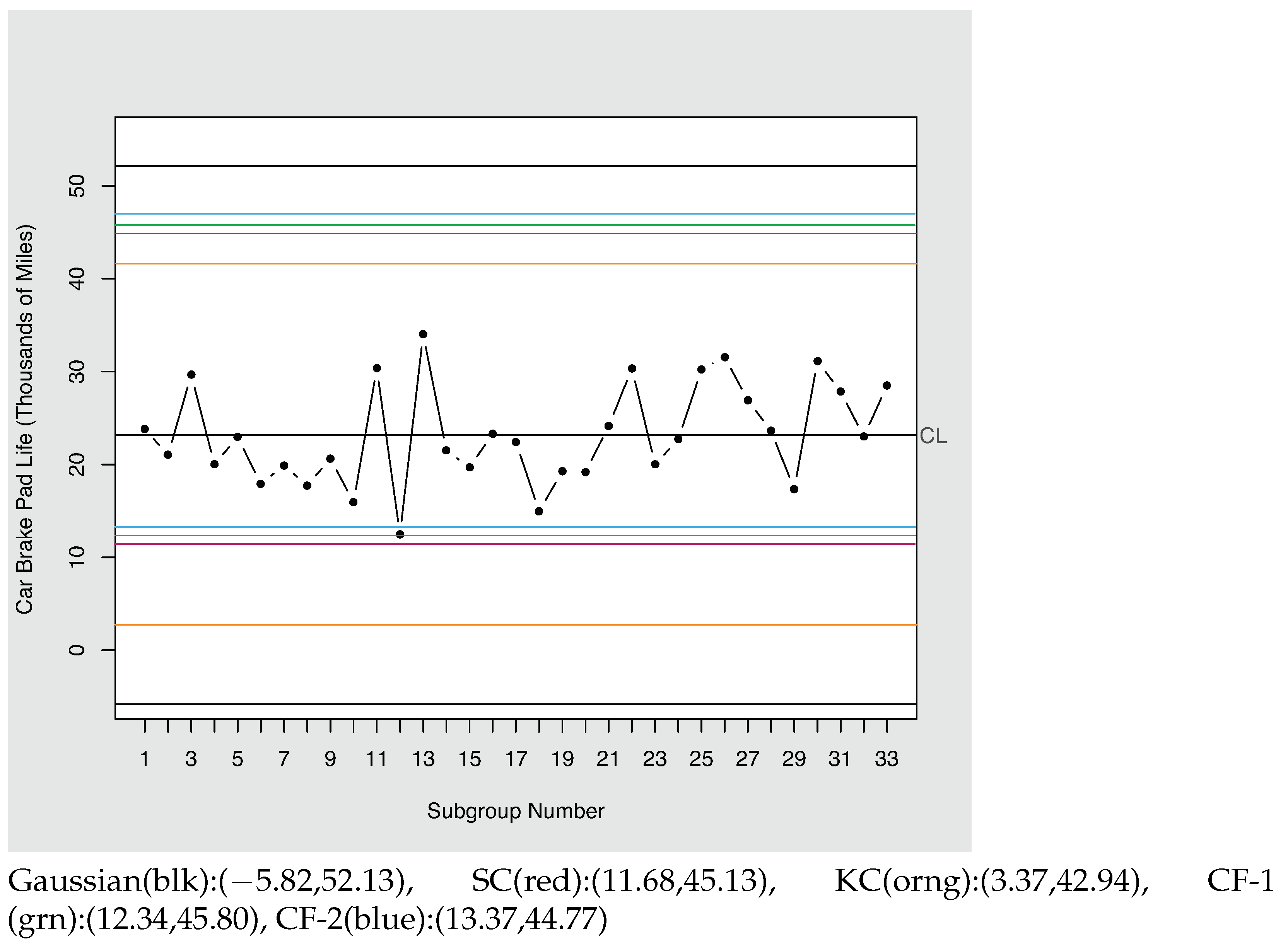
5. Control Charting Application

A dataset in which the lifetime of 98 randomly sampled car brake pads are reported in [20]. Assuming these were collected in subgroups of size $n=3$, the summary measures of the distribution of the sample mean were calculated according to Equation (13) and are given by $\widehat{\mu }=23.15145$, $\frac{\widehat{\sigma }}{\sqrt{3}}=5.57604$, $\frac{\widehat{{\nu }_3}}{\sqrt{3}}=0.7956$, and $\frac{\widehat{{\nu }_4}}{3}=0.6692$. A $\overline{X}$-chart with the sample data plotted against Gaussian/Shewhart, SC, KC, CF-1, and CF-2 limits is given in Figure 5.

Upon inspection of this control chart, the Gaussian/Shewhart limits do not account for either the skewness or kurtosis in the data and are, hence, very wide. The KC limits capture the effect of kurtosis and are hence a bit more narrow, yet are symmetrical about the mean without adjustment for skewness. The LCL of the SC, CF-1, and CF-2 limits is progressively larger in magnitude and, hence, the SC limits do not flag the mean of the 12th subgroup as being out-of-control, whereas the CF-1 limits have this point on the boundary and the CF-2 limits signal an out-of-control condition. Hence, the sensitivity of the control chart is increased as more complete information about the measures of the distribution of the sample mean is included in the control limit calculation.

6. Discussion

This research contributes to the study of control charts for the mean of a process in which the skewness and kurtosis of the population distribution are non-negligible. Cornish–Fisher approximations provide a closed form UCL and LCL for small sample sizes inclusive of skewness for the CF-1 expansion and inclusive of skewness and kurtosis for the CF-2 expansion. The approximation is distribution independent and was shown to be fairly robust to errors in estimating these measures from data. They outperform the similarly derived limits for the SC and KC methods that incorporate smoothing function in ARL performance, and do not require extraneous parameter specifications, such as the WSD and IEWMA methods. In summary, the CF-1 and CF-2 limits represent an improvement over previous research because they are closed form, inclusive of skewness and kurtosis, distribution independent, and accurate at small sample sizes. While there are some limitations to the use of these limits based on the domain of validity constraints on the skewness and kurtosis measure, it is noted that this constraint is quite large when considering the distribution of the mean when sub-grouping, and that the control limits do not cease to exist outside this domain of validity, but rather lose accuracy.

We propose future research into the domain of validity and how to address this limitation, including some research by [21] on using rearrangement. Future work also includes investigating methods to overcome the shortcomings of the domain of validity on skewness and kurtosis values set for a second order truncated Cornish–Fisher expansion series. This could involve exploration on possible additional functions to incorporate into the approximations of the control limits to ensure stability of the series expansion. Another possibility is investigating higher orders of truncation at the 3rd and 4th order, which would change the domain of validity by including higher order expansions into the approximation. Finally, applications beyond quality control could be investigated in which generally approximating the convolution of sums or averages are necessary.

7. Conclusions

This paper presents control limits for monitoring the mean of a process based on first and second order Cornish–Fisher expansions that are inclusive of the skewness and kurtosis measures of a population distribution. The theoretical accuracy of these limits in the case in which the skewness and kurtosis measures are known was shown to be a major improvement over traditional Shewhart limits based in the central limit theorem, and over other limit approximation methods that are inclusive of these measures in their specification. A simulation study showed that Cornish–Fisher limits are both accurate and consistent in practice, when these measures are estimated from even a limited amount of pre-sampled data. An $\overline{X}$ control chart was derived using an array of limit approximations for a real-world dataset, showing a comparative practical application of this methodology.

References

1. Zain, Z.; Yahaya, S.S.S.; Ahmad, N.; Atta, A.M.A. New X-bar Control Chart Using Skewness Correction Method for skewed Distributions with Application in Healthcare. Syst. Rev. Pharm. 2020, 11, 120–131. [Google Scholar]
2. Dreves, M.; Huang, G.; Peng, Z.; Polyzotis, N.; Rosen, E.; Suganthan, G.C.P. From Data to Models and Back. In Proceedings of the Fourth International Workshop on Data Management for End-to-End Machine Learning, Portland, OR, USA, 14 June 2020; pp. 1–4. [Google Scholar]
3. Mehta, R. Self-Assessment Data May Be Significantly Skewed During Global Health Crises. Int. J. Aviat. Res. 2020, 12. [Google Scholar]
4. Chan, L.K.; Cui, H.J. Skewness Correction X ¯ and R Charts for Skewed Distributions. Nav. Res. Logist. 2003, 50, 555–573. [Google Scholar] [CrossRef]
5. Tadikamalla, P.; Popescu, D. Kurtosis Correction Method for X ¯ and R ¯ Control Charts for Long-Tailed Symmetrical Distributions. Nav. Res. Logist. 2007, 54, 371–384. [Google Scholar] [CrossRef]
6. Maillard, D. A User’s Guide to the Cornish Fisher Expansion; SSRN:1997178 2018; pp. 1–14. Available online: https://papers.ssrn.com/sol3/papers.cfm?abstract_id=1997178 (accessed on 12 April 2022).
7. Blanca, M.J.; Arnau, J.; López-Montiel, D.; Bono, R.; Bendayan, R. Skewness and Kurtosis in Real Data Samples. Methodology 2013, 9, 78–84. [Google Scholar]
8. Bai, D.S.; Choi, S.I. X ¯ and R control charts for skewed populations. J. Qual. Technol. 1995, 27, 120–131. [Google Scholar] [CrossRef]
9. Shu, L.; Wei, J.; Wu, J. A one-sided EWMA control chart for monitoring process means. Commun. Stat. Comput. 2007, 36, 901–920. [Google Scholar] [CrossRef]
10. Jones, A. The statistical design of EWMA control charts with estimated parameters. J. Qual. Technol. 2002, 34, 277–288. [Google Scholar] [CrossRef]
11. Jensen, A.; Jones-Farmer, A.; Champ., C.; Woodall, W. Effects of parameter estimation on control chart properties: A literature review. J. Qual. Technol. 2006, 38, 349–364. [Google Scholar] [CrossRef]
12. Chakraborti, S. Nonparametric (distribution-free) quality control charts. Encycl. Stat. Sci. 2011, 1–27. [Google Scholar] [CrossRef]
13. Chakraborti, S.; Graham, M. Nonparametric (distribution-free) control charts: An updated overview and some results. Qual. Eng. 2019, 31, 1–22. [Google Scholar] [CrossRef]
14. Jones-Farmer, L.A.; Jordan, V.; Champ, C.W. Distribution-free Phase I control charts for subgroup location. J. Qual. Technol. 2009, 41, 304–316. [Google Scholar] [CrossRef]
15. Gibbons, J.D.; Chakraborti, S. Nonparametric Statistical Inference, 5th ed.; Taylor and Francis: Abingdon, UK, 2010. [Google Scholar]
16. Amin, R.W.; Reynolds, M.R.; Bakir, S.T. Nonparametric quality control charts based on the sign statistic. Commun. Stat. Theory Methods 1995, 24, 1597–1623. [Google Scholar] [CrossRef]
17. Bakir, S.T. A distribution-free Shewhart quality control chart based on signed-ranks. Qual. Eng. 2004, 16, 613–623. [Google Scholar] [CrossRef]
18. Cornish, E.A.; Fisher, R.A. Moments and Cumulants in the Specifications of Distributions. Rev. Int. Stat. Inst. 1937, 4, 1–14. [Google Scholar] [CrossRef] [Green Version]
19. Johnson, N.; Kotz, S. Continuous Univariate Distributions; Wiley: New York, NY, USA, 1970; p. 34. [Google Scholar]
20. Omar, M.; Arafat, S.; Hossain, M.; Riaz, M. Inverse Maxwell Distribution and Statistical Process Control: An Efficient Approach for Monitoring Positively Skewed Process. Symmetry 2021, 13, 189. [Google Scholar] [CrossRef]
21. Chernozhukov, V.; Fernandez-Val, I.; Galichon, A. Improving point and interval estimators of monotone functions by rearrangement. Biometrika 2009, 96, 559. [Google Scholar]
Figure 1. Domain of validity for skewness and kurtosis values for the second order Cornish Fisher Expansion.
Symmetry 14 01176 g001
Figure 2. G a m m a ( n γ , 1 n λ = 3 ) probability distributions of varied shape and skew used in performance analysis and representing the range of many control chart applications.
Symmetry 14 01176 g002
Figure 3. Operating characteristic (OC) curves of an X ¯ chart with subgroups of size n for a G a m m a ( γ , 1 λ = 3 ) population distribution with shifted shape parameter γ = γ 1 , where γ = γ 0 is the in-control case.
Symmetry 14 01176 g003
Figure 4. Operating characteristic (OC) curves of an X ¯ chart with subgroups of size n for a G a m m a ( γ , 1 λ ) population distribution with shifted scale parameter 1 λ = 1 λ 1 , where 1 λ = 1 λ 0 = 3 is the in-control case.
Symmetry 14 01176 g004
Figure 5. X ¯ Control Chart limits for car brake pad lifetime data ( m = 33 , n = 3 ).
Symmetry 14 01176 g005