1. Introduction
Keeping cities safe is a challenge for the police, especially when crime increases in all its forms. People live in fear and feel insecure. Factors such as the environment, social network gossip, interpersonal communication with neighbors, relatives, and lack of policies in an area can alter the insecurity perception [
1].
People who have not been victims of crime can fear crime just as much as people who have suffered it, the latter people being affected psychologically by the perception of insecurity [
2]. According to the statistics of the National Institute of Statistics and Geography (INEGI) [
3] in 2020, women had a higher perception of insecurity with 72.7%, while men had scored 62% in insecurity perception. Additionally, from INEGI 2016, the most common crimes in México are extortion, vehicle theft, assault, burglary, and robbery on public roads and transportation. These crimes’ frequencies decreased compared to 2020, caused by the SARS-CoV-2 pandemic (COVID-19), because people stayed in their homes, which caused an increase in extortion and domestic violence.
Delinquency is a problem prevalent in countries in Latin America because of their high level of violence. To measure the delinquency level, some countries gather information from police databases, and others such as Norway, Denmark, Sweden, and Finland carry out surveys to know the safety perception of their people when going out on the street, to implement strategies [
4].
Because of delinquency, governments lose credibility, and societies suffering from this problem tend to refrain from voting, as they do not see government intervention to stop crime rising [
5].
Education and poverty are some factors that influence delinquency, from a study conducted by Millán-Valenzuela et al. [
6] in Italy and México. This study showed that the areas with greater economic prosperity have the highest crime rates compared to some states where poverty is extreme. On the other hand, it is possible to assume that delinquency and education are closely related; commonly, young people who drop out or with low levels of education engage in crime. Hence, a country with a more educated society is less prone to experiencing problems such as poverty and delinquency. Therefore, education would be a good crime prevention measure.
Latin America has the world’s highest crime rate, according to Díaz et al. [
7]. Some helpful prevention strategies are: monitoring crime, diseases, and new criminal organizations; updating criminal sanctions; prison expansion; and making neighborhood meetings so that neighbors get to know each other and are more united.
To collect criminal information not kept in police databases, countries from central and eastern Europe, Africa, Latin America, and Asia conducted a series of surveys, asking people about their experiences with crime. These surveys were carried out in 2000 by the international study on criminal victims, supported by the united nations interregional institute.
As a result, more information was obtained than is available in police databases; this is because sometimes crimes are not reported, out of fear, shame, or because people know there is police mismanagement or corruption, which causes more crime. Furthermore, they found that criminal activity predominates in densely populated cities, i.e., because the city’s services are not enough for their number of inhabitants. Additionally, the lack of work, education, and housing, among other factors, lead to crimes [
8].
The prevention of criminal activity has been tackled through several predictions and forecasting methods, including regression models and machine learning.
This paper proposes a study forecasting crime with a short series of four crimes with eight forecasting methods applied to thirty-five small-sized real crime time series. Furthermore, we propose five forecasting techniques that use the seasonal component of the time series. Additionally, we compare the performance of classical and machine-learning-based ensemble methods and analyze the impact of the seasonal component of the time series in the forecasting techniques. Finally, we compared the rankings of the Average sMAPE and the Mean Rank of a Friedman test and found slight variations in the rankings of the forecasting methods and techniques. However, both maintain the same behavior.
The remainder of this paper is structured as follows:
Section 2 shows the state of the art regarding prediction and crime forecasting. In
Section 3, we describe the models and methods used to produce and process the short-sized time series, which includes data extraction and preparation.
Section 4 shows the computational results of the experimentation configurations. Finally,
Section 5 and
Section 6 show the discussions of the findings and the conclusions, respectively.
2. State of the Art of Crime Forecasting
Commonly, crimes are committed in groups because doing this makes them easier, making it necessary to identify the criminal gang based on criminal history, location, dates, and other variables considered essential for this study. Implementing techniques such as regressive models, neural networks, time series methods, and hybrid models has improved the forecasting or behavior prediction of these gangs or places that could be affected by crime.
Some studies using artificial intelligence have made successful predictions such as Ordóñez et al. [
9], who used support vector machines. They applied a linear regression to predict the proximity of the values and obtain the proximity to the highest point of committed robberies in a specific year. They produced two models and compared their prediction accuracies using the squared error.
Cichosz [
10] proposed a crime risk prediction focused on urban areas using logic regression, support vector machine, decision trees, and Random Forest. For this study, the author took information from a London database, focused on geographic data from Manchester, Liverpool, Bournemouth, and Wakefield, considering antisocial behavior, the rate of sexual crimes, robbery with violence, shoplifting, and other types of robbery and theft.
Another tool used in crime prediction is deep neural networks. In [
11], Chun et al. used this technique to predict the number of crimes using data from 1997 to 2017, considering the type of crime, severity level, and the number of faced charges. They used a criminal code, gender, age, race, and record date. This information successfully predicted the criminality level based on the record of each person for five years, labeling the crime from 0 to 3, depending on the severity. They identify that when the prediction finds a high-level crime, the probability of this crime is taken for granted for the next few years.
Wang et al. [
12] used ARIMA with information from a London police database to carry out prediction research based on historical data from 2016 to 2018 for analysis and predictions using ARIMA with fourteen different types of crimes. Liu and Lu [
13] used a hybrid model and STARMA model with LSTM for San Francisco’s crime prediction using the United States historic data from 2003 to 2017. From this database, the authors used the number of incidents, description, day of the week, date, time, resolution, district, and location,
X,
Y. Their best model was a hybrid model which incorporates improvements to adapt to the data, adding a linear function and improving the accuracy to forecast the numbers of crimes committed for a specific hour, day, week, month, or year.
With criminal data from India, Jha et al. [
14] made a comparison of ARIMA, neural networks, and machine learning. For this study, ARIMA models produce better results than the other methods.
Yadav and Kumari [
15] used autoregressive models and fuzzy membership functions for multivariate crime predictions. They used a dataset from Delhi city in India for the following crimes: vehicular crime, arson, assaults, kidnappings, robberies, theft, and violent assault. They found that the fuzzy membership simplified multivariate crime prediction.
Shi et al. [
16] conducted a study of an ARMAX model applied to US crimes related to age, the period of the committed crime, and similar characteristics regarding the offender. These characteristics help identify the trend of crime and the relationship with other planned crimes, among others presented in each case.
Melgarejo et al. [
17] used two different databases, the first from San Francisco regarding burglary crime and the second from Colombia regarding cellphone theft. The authors used clustering algorithms to study the dynamics of criminal groups to produce time series. Additionally, they identified criminal gangs, minimizing the fuzzy partition index and generating fuzzy evolutionary predictors. Finally, they found that this clustering improved the time series to enhance crime predictions with non-linear analysis.
On the other hand, Izonin et al. [
18] and Tkachenko et al. [
19] tackled the problem of processing short datasets and missing values from a regression perspective. They used techniques such as support vector regression with kernels, adaptive boosting and stochastic gradient descent, neural networks, multilayer perceptron, and random forest. The authors have a medical dataset to predict calcium concentration in human urine and air pollution monitoring data, respectively.
3. Models and Methods
This section includes the data extraction, preparation and the experimentation methodology. All these processes were carried out using R.
3.1. Data Extraction
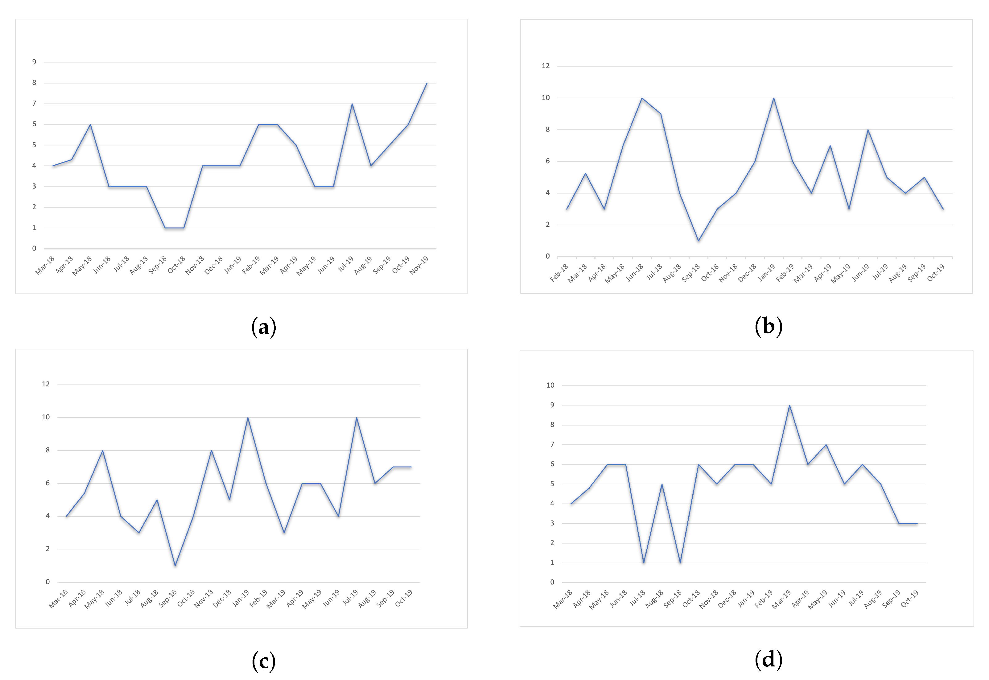
First, we built the time series using surveys of the frequency of each crime in several sectors of each city. These sectors respond to each city’s socioeconomic, demographic, and geographic aspects. Then, we condensed this information producing thirty-five series ranging in size from fourteen to twenty-one observations.
3.2. Data Preparation
Additionally, we noticed that every series had an outlier value in the second element; therefore, we changed that value with the average value of the series.
Finally, we conducted some preliminary experiments and noticed that several series produce a symmetric mean average percentage error (sMAPE) of 200; this happened because of zero values in the series. Therefore, we increase every value of all the time series by one to avoid this issue.
Figure 1 shows a time series example for each one of the four types of crime.
3.3. Forecasting Methods
In this section, we show the methods used to forecast.
We use four simple forecasting methods: ARIMA, Holt–Winters (HW), Artificial Neural Networks (ANN), and Simple Moving Averages (SMA).
Additionally, we used four state-of-the-art forecasting methods: Jaganathan, which achieves the fourth place in the M4 competitions (Makridakis) [
20]; FFORMA, which is at second place in M4; Hybrid, which is a simple hybrid forecasting method; and LightGBM, whose performance achieved first place in M5 competition [
21].
These last four forecasting methods use the following components:
-
[Jaganathan] combines numerous statistical and machine learning methods [
22]: naive/snaive; ExponenTial Smoothing (ETS); dampened ETS; bagged ETS; exponential smoothing, complex exponential smoothing, general exponential smoothing; multi-aggregation prediction algorithm (MAPA); temporal hierarchical forecasting; autoregressive integrated moving average (ARIMA); ThetaH; hybrid Theta; forecast pro; seasonal and trend decomposition using loess forecast; trigonometric Box–Cox transform, ARMA errors, trend and seasonal components (TBATS); double seasonal Holt-Winters; and multilayer perceptron and extreme learning machines.
-
[FFORMA] uses the following forecasting methods [
23]: naive, random walk with drift, seasonal naive, theta method, automated ARIMA algorithm, ETS, TBATS, STLM-AR seasonal and trend decomposition, and neural network time series forecasts (NNETAR).
-
[Hybrid] ensembles [
24]: auto ARIMA, ETS, Theta, NNETAR, seasonal and trend decomposition using loess, TBATS, snaive.
-
[LightGBM] [
21] applies decision trees.
3.4. Proposed Forecasting Techniques
For every forecasting method, we propose five different forecasting techniques.
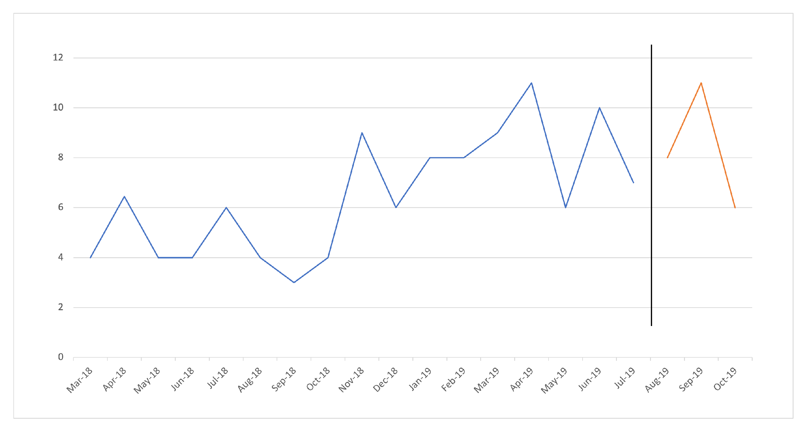
Re is the regular forecasting of the training section of the series, ARIMA, HW, ANN, SMA, Jaganathan, FFORMA, Hybrid, or LightGBM (see
Figure 3); see Equation (
1).
where the Forecasting_Method is any of the previously presented forecasting methods, and
series is the training section of the time series.
We made preliminary forecasting tests and found that several forecasting methods performed poorly. To improve the forecasting, we used a Fourier decomposition as suggested by Hyndman in [
25,
26,
27] to decompose a time series in trend, seasonal, and residuals.
The following techniques use a Fourier decomposition to extract the seasonal component of the train section of a series; for simplicity, we will use the term seasonal component.
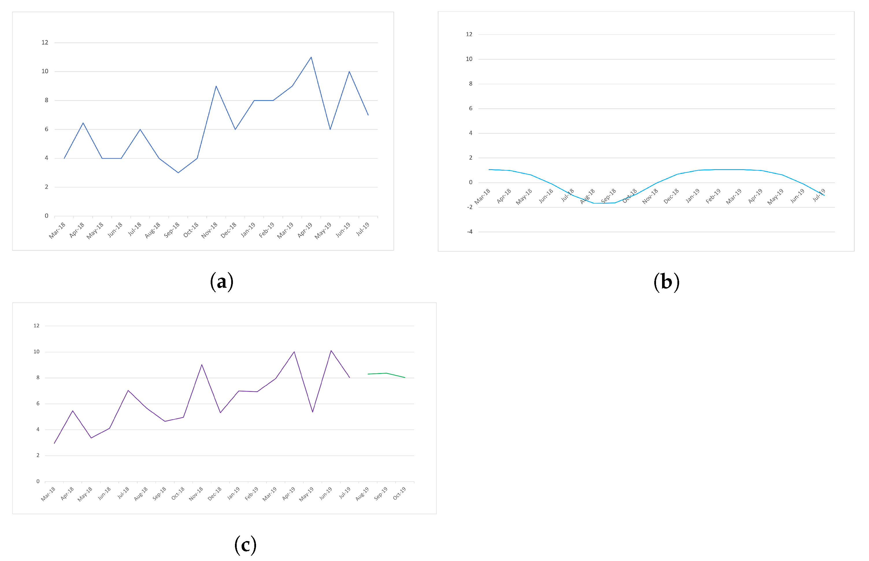
ReMS is the regular forecasting of the series minus the seasonal component.
Figure 4 shows this technique’s scheme, where
Figure 4a shows the train section of the series,
Figure 4b is the seasonal component and
Figure 4c shows the forecasting of
Figure 4a minus
Figure 4b, see Equations (
2)–(
4).
where
seriesMS is the training section of the time series minus the
seasonal component.
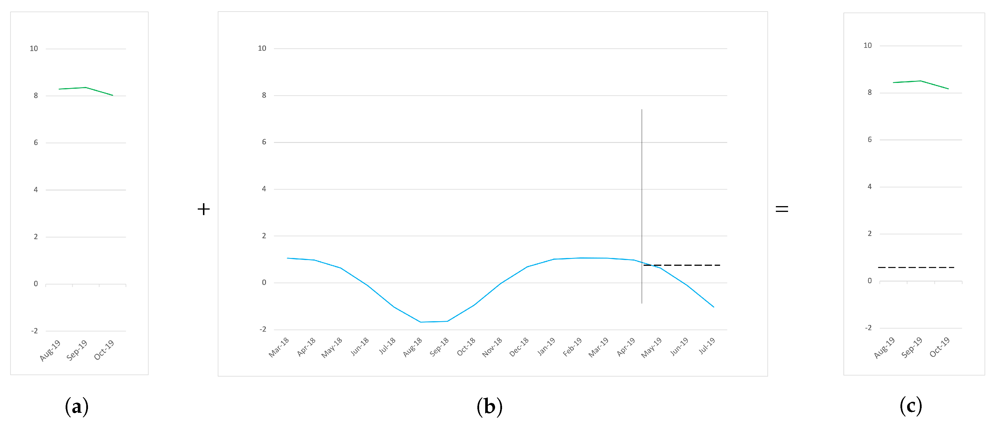
The CAS technique is a composed forecasting of the ReMS plus the average of the whole seasonal component (see
Figure 5). Here, we use the forecasting of ReMs (
Figure 5a) and add the average of the seasonal component (
Figure 5b) to produce the final forecasting (
Figure 5b); see Equation (
5).
CAHS is the same as CAS, but instead of using the average of the whole seasonal component, we use the average of the last
h values of the seasonal component (see
Figure 6). We propose this variation to highlight the latest tendencies of the seasonal component shown in
Figure 6b, to increase or decrease the ReMS forecasting (
Figure 6a) to produce the new CAHS forecast in
Figure 6c; see Equation (
6).
where
is a fragment of
that contains its last
h elements.
Figure 7 shows the CReMSPlusFS scheme. This forecasting technique uses the ReMS (
Figure 7a) and adds the independent forecasting of the seasonal component (
Figure 7b), to yield a combined forecasting (
Figure 7c). It is important to highlight that both forecastings are produced using the same forecasting method; see Equation (
7).
where the Forecasting_Method is the same for both components.
Therefore, we use eight forecasting methods and five forecasting techniques for each one, producing forty experimentation configurations.
4. Experimental Result
In this section, we present the results of the forty experimentation configurations applying the symmetric mean average percentage error (sMAPE) used in M4 competitions [
20] and the Mean Rank of the Friedman nonparametric test.
Table 1 shows the forecasting methods and techniques in columns one and two, which are ordered according to the Average sMAPE in column three. Here, we can see that the forecasting method that produces the best average sMAPE is ARIMA, followed by Jaganathan, SMA, and Hybrid, while the first three use Re as forecasting technique. These methods continue until the fifteenth forecasting method, which is the FFORMA. On the other hand, the last positions correspond to ANN, LightGBM, and HW with the CReMSPlusFS technique.
Finally,
Table 2 adds the Mean Rank of a non-parametric Friedman Test to
Table 1 in column three, which ranks the experimental configuration (the pair of forecasting method and technique). Additionally, we included a fifth column that shows, for every experimental configuration, the position changes shown in
Table 1. Here, we can see that some experimental configurations change ranks by several units; however, the general performance remains the same. We consider the mean rank of the Friedman test to be more reliable than the average sMAPE, given that it was designed for statistical comparisons.
Now, we can see that the first forecasting method is SMA followed by ARIMA, Hybrid, and Jaganathan until the fourteenth experimentation configuration with FFORMA. The last forecasting methods are LightGBM, ANN, and HW mixed with ARIMA. We can see that SMA CAHS, SMA ReMS, and SMA CAS have increased their rankings, to positions thirteen ( ↑ × 13), five ( ↑× 5), and five ( ↑× 5), respectively, highlighting that the forecasting methods with the most variations are in the top rankings.
5. Discussion
We suspect that ANN and LightGBM produce the highest sMAPE and worst Mean Rank because they did not have enough training data to identify consistent patterns for the forecasting. Furthermore, HW uses exponential smoothing and works with the seasonal component. It is important to highlight that given the size of the time series, we consider that it is hard to identify the seasonal component correctly, which might lead to a poor performance.
On the other hand, SMA does not use complex parameters nor the seasonal component; it only requires the last values to conduct the forecasting. Furthermore, ARIMA models try to describe the autocorrelations in the data, and it is composed of a combination of differencing with autoregression and a moving average model; these parts are described by the
p,
d and
q parameters, respectively, in ARMIA (
). It is important to highlight that 85% of the total time series were classified as white noise by ARIMA [
28], meaning that they lack autocorrelation and have high levels of symmetry by having a uniform distribution of data, similar to a random walk process [
26]. Therefore, it is difficult to forecast these series because they have the same probability for the series to go up or down.
These time series used the model ARIMA (0,0,0), which forecasts a straight line with the value of the average of the whole time series, similar to SMA. Additionally, ARIMA can produce different models, leading to variations in its performance.
Additionally, Hybrid and Jaganathan also exhibited good performances but not enough to be called the best, and according to the parsimony principle, if several forecasting methods exhibit similar performances, we should use the simplest among them.
Regarding the forecasting techniques, most of the best five methods tend to disregard the seasonal component, whether ignoring it completely (ReMS) or using only its average (CAS) or a fragment of it (CAHS).
6. Conclusions
In this paper, we tackle the problem of forecasting short-sized crime time series for common crimes (theft, shoplifting, vehicular, and burglary) in several sectors of three cities of Tamaulipas, México. For this problem, we propose the use of simple and machine-learning-based ensemble methods. Additionally, for each one of the forecasting methods, we propose five different forecasting techniques that imply the extraction of the seasonal component of the series, producing a total of forty experimentation configurations.
We rank the experimentation configurations using two criteria, the average sMAPE and the mean rank of the Friedman test. As expected, both rankings produce different orders but with the same pattern, i.e., SMA, ARIMA, Hybrid, and Jaganathan as the best forecasting methods and LightGBM, ANN, and HW as the methods with the lowest performance, leaving FFORMA in the middle.
The best five experimentation configurations tend to dismiss the seasonal component CAHS, ReMS, and CAS. As stated before in
Section 5, most of the internal configurations of ARIMA tend to forecast using a simple average of the whole series, ignoring the seasonal component even if it uses the Re forecasting technique. Finally, the worst experimentation configurations use the series with the seasonal (Re) or forecast the seasonal and add it to the forecasting of the series minus the seasonal (CReMSPlusFS).
Therefore, for this study, we can conclude that the best-performing forecasting methods, starting with the best, are SMA, ARIMA, Hybrid, and Jaganathan. In contrast, the worst forecasting methods are LightGBM and ANN. The best forecasting techniques tend to disregard the seasonal component. Furthermore, SMA, Hybrid, FFORMA, HW, ANN, and LightGBM tend to exhibit their best performances by ignoring the seasonal component and their worst otherwise, whereas Jaganathan and ARIMA have an inverse relationship regarding the use of the seasonal component. However, the internal components of ARIMA identify most of the time series as white noise (no autocorrelation and high symmetry), ignoring the seasonal by generating models ARIMA (0,0,0). Moreover, Jaganathan also uses ARIMA as part of its components; hence, we consider it to work similarly.
It is important to remember that these results hold for small-sized time series, and might be specific to these kind of time series. In future work, we recommend using other techniques that involve the tendency and residuals, as well as the development of hyper-heuristics to find better forecasting techniques and the use of a larger set of time series.


 ,
, 


