Conditioned Adaptive Control for an Uncertain Bioreactor with Input Saturation and Steep Settling Desired Output

Abstract

In this work, a controller is developed for a continuous bioreactor with an unknown reaction rate term, subject to input saturation. The substrate concentration and the dilution rate are chosen as output and input, respectively. The controller formulation and the stability analysis are performed by the theory of dead zone Lyapunov functions, Lyapunov stability, and model reference adaptive control. As the main results, the dynamics of the Lyapunov function is determined separately for saturation and non-saturation events, and then a unified expression is deduced. In addition, the asymptotic convergence of the tracking error and boundedness of updated parameters are determined for the whole closed loop regime encompassing saturation and non-saturation events, and also for input saturation events, as a function of the terms and parameters of the reference and system models. The main contributions over closely related control designs, are (i) the effect of input constraint limits and desired output on the convergence of the tracking error during input saturation events are determined, considering settling behavior of the desired output with a steep section; (ii) the upper limit of the input constraint that guarantees output convergence during input saturation events is determined as function of the model terms, but independently of the time derivative of the desired output and its limit; (iii) a new dead zone Lyapunov function is proposed which allows proving asymptotic convergence of the tracking error during input saturation events in the presence of a fast variation in the desired output. Finally, the effectiveness and advantages of the developed controller are illustrated by simulation.

1. Introduction

In process control using integral action, input saturation events may lead to severe degradation of the closed loop performance, for instance, in continuously stirred tank reactors [1], exothermic tubular reactors [2], and bioreactors [3,4,5]. Different antiwindup strategies are commonly used to this end [6]. In the case of adaptive control involving update laws, an excessive increase in the updated parameters may occur, causing degradation of the closed-loop behavior [7,8,9,10,11]. This effect is commonly tackled by using the auxiliary system strategy, which was originally known as the augmented error signal (AES) strategy, in which an auxiliary system is employed to tackle the effect of input saturation. In adaptive controllers with AES strategy, the avoidance of an excessive increase in updated parameters, and the convergence of the modified tracking error asymptotically to a compact set of small size (see [9,11,12,13,14,15,16,17,18]) is guaranteed.

Some recent adaptive AES-based control designs are discussed in what follows, in which an auxiliary system is used to tackle the effect of input saturation. In [17], an adaptive tracking controller was designed for nonlinear systems with input saturation, using barrier positive functions. Nonlinear systems in a strict feedback form with unknown dynamics were considered. In [11], an adaptive sliding mode controller was designed for uncertain Eule–Lagrange systems with input saturation. A leakage-type adaptive law was used to tackle the lack of knowledge on the disturbance terms. Simulations for a two-link robot manipulator showed that the designed controller reduces the chattering effect in the control input compared to a conventional sliding mode controller.

Some AES control designs with application to bioreactors are discussed in the following. In [14], an observer-based nonlinear controller was designed for a class of single input single output (SISO) systems in the general strict feedback form, subject to input saturation. The adaptive backstepping was used as the control framework, and the AES strategy was used for tackling input saturation. In the continuous bioreactor application, the feed substrate and reactor biomass concentrations were defined as input and output, respectively. In [19], an observer-based adaptive fuzzy controller was designed for a class of SISO nonlinear systems with unknown dynamics, and unknown control gain, subject to input saturation. The adaptive backstepping is used as a control framework, and the AES strategy was used for tackling the input saturation. The controller was applied to a system of two series continuously stirred isothermal tank reactors. The inlet reactant concentration was the manipulated input, and the outlet reactant concentration was the output. In [13], an observer-based controller was designed for a SISO nonlinear time-delay system subject to asymmetric input saturation and external disturbances. The controller was applied to a system of two series isothermal continuously stirred tank reactors. The substrate or reactant concentration in the feed to the first CSTR was the manipulated input, and the product concentration in the outlet of the second CSTR was the output.

In adaptive control with an AES strategy, the states are modified through the addition of auxiliary variables. From the stability analysis, it follows that: the states and updated parameters are globally bounded; the excessive increase in updated parameters is avoided is guaranteed; the modified tracking error asymptotically converges to a compact set of small size; the tracking error asymptotically converges to a compact set that is a function of the error of input saturation and the control design parameters (see [11,12,14,15,17]). In addition, the bounds of the transient response of the Lyapunov function and tracking error or modified tracking error depend on: (i) the parameters of the control law, update law, observer and auxiliary systems; (ii) the upper bound of disturbance terms or model terms and parameters. In this way, the differentiated effect of the input constraint limits, model terms, and input constraint limits on either the convergence or transient response of the output error during input saturation events is not provided (see [11,12,14,15,16]). An alternative approach to handle the effect of input saturation is to study the stability with separate consideration of the input saturation and no input saturation events [20]. Therein, a novel robust feedback controller was designed for a second-order system subject to input saturation, disturbances, and model uncertainties. The control design was based on a sliding control approach, with twisting and continuous twisting algorithms. The global finite-time stability properties of the closed-loop system were determined via the Lyapunov function. A set of controller parameters was proposed, based on the convergence properties.

In this work, a controller is formulated for a continuous bioreactor subject to input saturation, considering the input saturation events and desired output featuring settling behavior with a steep section. The asymptotic convergence of the tracking error to a compact set of user-defined width and parameter boundedness is guaranteed. The substrate concentration and the dilution rate are chosen as output and input, respectively. The asymptotic convergence of the tracking error during input saturation events is proved, as function of the terms and parameters of the reference and system models. The main contributions over closely related works are:

−

Contribution Ci. The effect of input constraint limits and desired output on the convergence of the tracking error during input saturation events is determined. In contrast, in current adaptive AES-based control (for instance [11,16,17,18]), the convergence of the tracking error is determined in terms of the controller parameters, not in terms of input constraint limits or desired out.

−

Contribution Cii. The upper limit of the input constraint guaranteeing output convergence during input saturation events is determined as a function of the model terms, but independent of the time derivative of the desired output and its limit. In contrast, this limit is not computed in common AES-based controllers (for instance [11,13,14,15,16,17,18,19]).

−

Contribution Ciii. Differently from [20], a new dead zone Lyapunov function is proposed which allows proving asymptotic convergence of the tracking error during input saturation events, considering desired output featuring settling behavior with a steep section.

The bioreactor model, reference model, control goal, and methods are provided in Section 2. The controller algorithm, the formulation of the controller, and the determination of the stability results are provided in Section 3. The numerical simulation is provided in Section 4, and the conclusions are drawn in Section 5.

2. Bioreactor Model, Reference Model, Control Goal, Materials and Methods

2.1. Bioreactor Model

Consider a continuous flow bioreactor described by the following model ([14,21,22,23]):

$$\frac{dX}{dt}=\left(\mu -D\right)X,$$

(1a)

$$\frac{dS}{dt}=\left(s_{in}-s\right)D-y_s\mu X.$$

(1b)

where $S$ is the substrate concentration; $X$ is the biomass concentration; $\mu$ is the specific growth rate; $y_s$ is the yields coefficient, $y_s\mu X$ is the substrate consumption rate; $S_{in}$ is the inflow substrate concentration; $D=Q_{in}/V$ is the dilution rate; $Q_{in}$ is the inlet flowrate, and $V$ is the volume of the culture medium. The output to be controlled is the substrate concentration $S$, and the control input is the dilution rate $D$.

The saturation of the plant input $D$ is:

$$D=\{\begin{array}{c}{D}_{max} if D_{cr}>D_{max} \\ D_{cr} if D_{cr}\in \left[D_{min} D_{max}\right]\\ D_{min} if D_{cr}<D_{min} \end{array},$$

(2)

where $D_{cr}$ is the control input signal to be designed, and $D_{min}$, $D_{max}$ are constant saturation bounds.

The following assumptions are considered:

Assumption 1.

The biomass and substrate concentrations feature $X\in \left(0, \infty \right)$,$S\in \left(0, S_{in}\right)$ ([23]).

Assumption 2.

The term $y_s\mu X$ is positive and inaccurately known or completely unknown, whereas the specific growth rate $\mu$ is bounded ([23]).

Assumption 3.

The values of$S$and$D$are known ([21,24]).

2.2. Control Goal and Reference Model

Control goal.

Consider the tracking error $e=S-y_d$, where $y_d$ is the desired output provided by the reference model ([25,26]):

$$\frac{d{y}_d}{dt}=-a_m{y}_d+a_{m}r,$$

(3)

where $r$ is the reference signal, and $a_m$ is a user-defined positive constant. The goal of the controller design is to formulate the control and update laws and to define the input constraint bound $D_{max}$, that achieve boundedness of the updated parameters and convergence of the tracking error $e$ to the compact set ${\mathsf{\Omega }}_e=\left\{e:\left|e\right|\le \epsilon \right\}$, where $\epsilon$ is positive, constant, and user-defined, considering a step type reference signal $r$, and moments of input saturation and no input saturation.

Remark 1.

The reference model (3) and the step type reference signal imply that the$y_d$signal is settling and may involve a steep section, whereas$d{y}_d/dt$is vanishing. The vanishing nature of$d{y}_d/dt$facilitates the controller design and avoids using large input saturation bounds that would be used to overcome large$d{y}_d/dt$values.

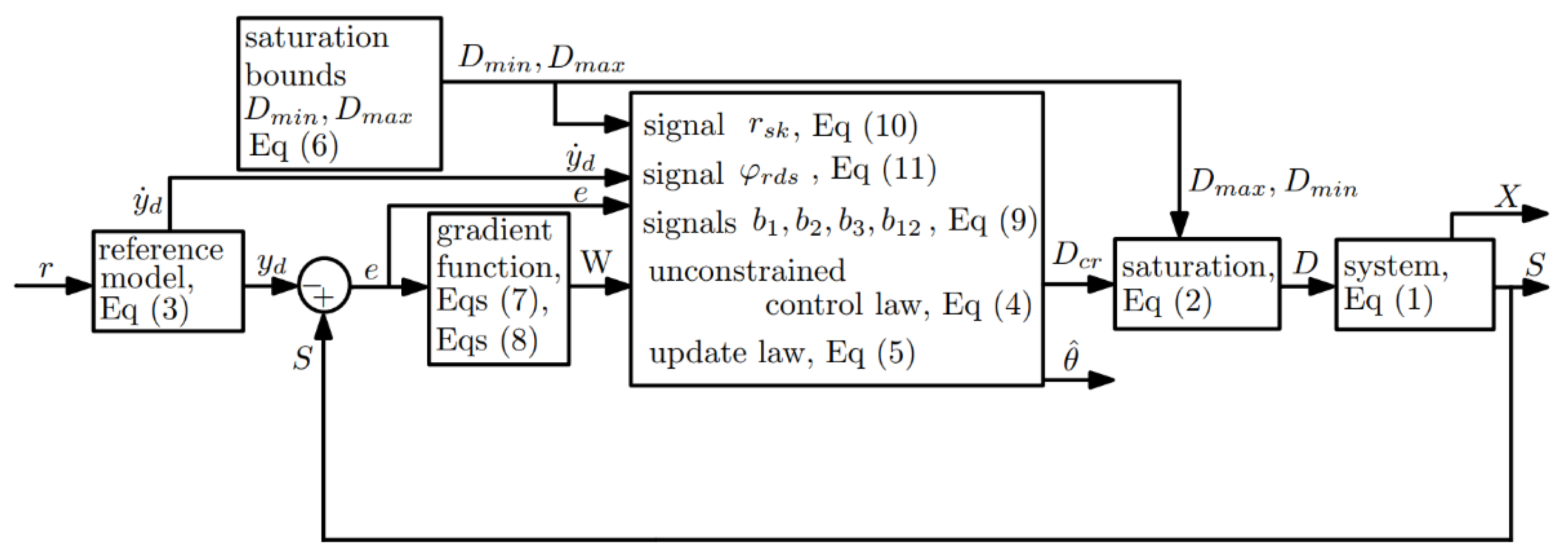
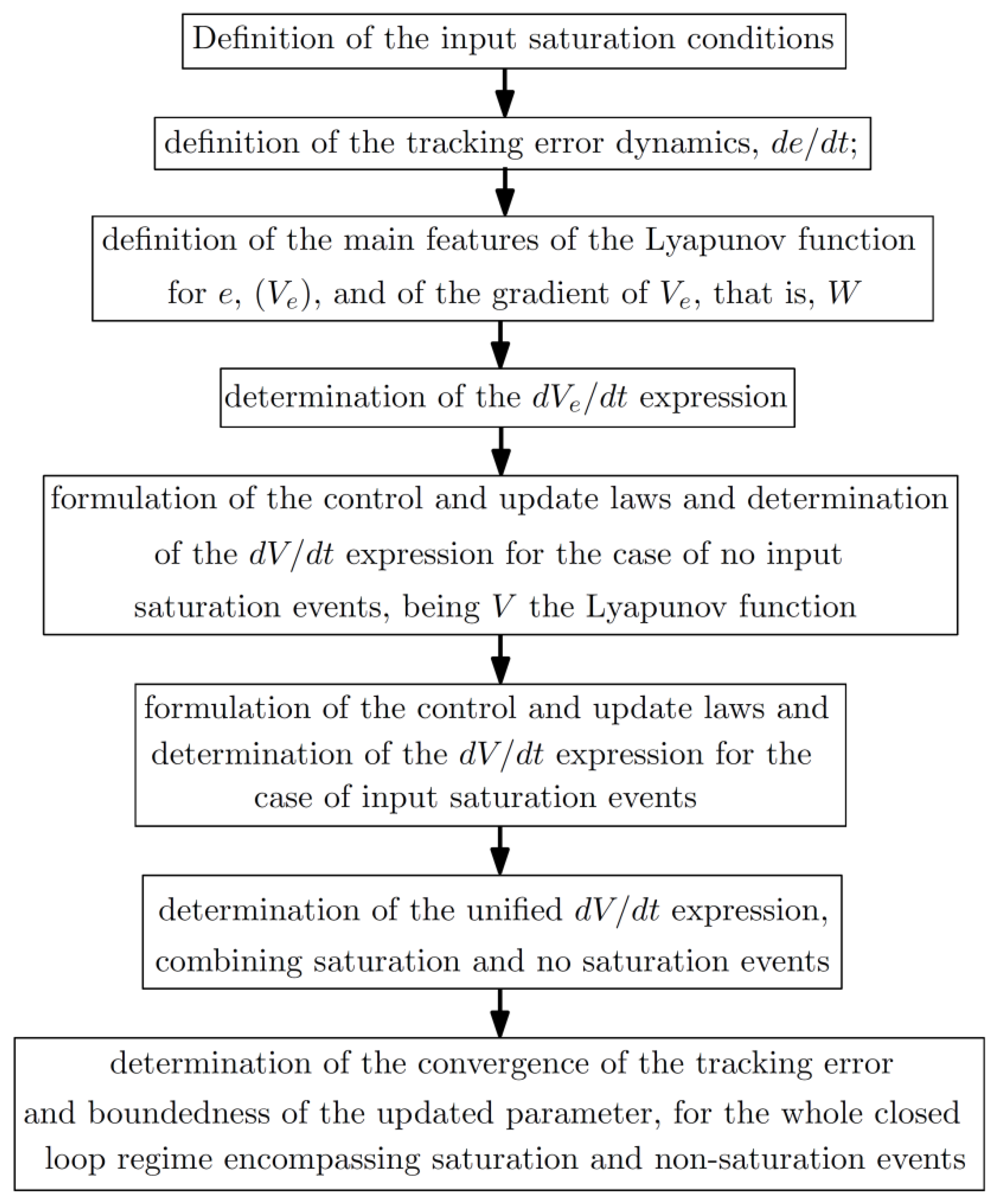
2.3. Materials and Methods: Overview of the Method for Control Design and Stability Analysis

The controller design and stability analysis considered a model for biomass and substrate concentrations (1), considering: (i) the model for biomass and substrate concentrations (1) subject to time varying inflow substrate concentration $S_{in}$, saturation of the input $D$ according to saturation condition (2); (ii) desired output $y_d$ given by the reference model (3), featuring time varying but settling behavior and high $d{y}_d/dt$ values during some time lapses. Both saturation and non-saturation events were considered. The main goals of the control design were: (i) to ensure convergence of the tracking error to a compact set whose width is user-defined; (ii) to ensure boundedness of the updated parameter $\widehat{\theta }$; (iii) to avoid discontinuous signals in the control signals.

The overall steps of the procedure are (see Figure 1):

−

Definition of the input saturation conditions;

−

Definition of the tracking error dynamics, $de/dt$;

−

Definition of the main features of the Lyapunov function for $e$, $\left(V_e\right)$, and of the gradient of $V_e$, that is, $W$;

−

Determination of the $d{V}_e/dt$ expression;

−

Formulation of the control and update laws and determination of the $dV/dt$ expression for the case of no input saturation events, being $V$ the Lyapunov function;

−

Formulation of the control and update laws and the determination of the $dV/dt$ expression for the case of input saturation events;

−

Determination of the unified $dV/dt$ expression, combining saturation and no saturation events;

−

Determination of the convergence of the tracking error and boundedness of the updated parameter, for the whole closed-loop regime encompassing saturation and non-saturation events.

The controller formulation and the stability analysis were performed by the theory of dead zone Lyapunov functions, Lyapunov stability, and model reference adaptive control. The controller design aimed at achieving non-positiveness features in the time derivative $dV/dt$, considering saturation and non-saturation events. Dead zone modifications were used in the Lyapunov functions with the following aims: (i) to facilitate the study of the convergence of the tracking error to a compact set whose width was user-defined and constant, (ii) to avoid the use of discontinuous signals in the controller design for no saturation moments. Dead-zone Lyapunov functions have been mainly used for robust control design. Early studies are presented in [25,27,28], and recent studies in [29,30,31,32,33].

The $dV/dt$ expression for the overall closed loop regime was obtained by combining that of the saturation events and that of the non-saturation events. During input saturation events the controller becomes an on–off type, so that it takes on either of the values $D_{max}$, $D_{min}$.

3. Control Algorithm, Controller Design, and Stability Analysis

In this section, the control algorithm, controller design, and stability analysis are presented, including the results mentioned as contributions in the Introduction, that is:

−

The asymptotic convergence of the tracking error $e$ to the compact set ${\mathsf{\Omega }}_e=\left\{e:\left|e\right|\le \epsilon \right\}$ is guaranteed, during the whole closed-loop regime in presence of input saturation events, and also it is guaranteed during input saturation events, considering high $d{y}_d/dt$ values occurring during some time lapses.

−

The condition for computing the limit for the input constraint $D_{max}$ is determined, which leads to asymptotic convergence of the tracking error in presence of input saturation events and is independent of $d{y}_d/dt$.

−

A new dead zone Lyapunov function is proposed which allows proving the asymptotic convergence of the tracking error during input saturation events, considering desired output featuring settling behavior with a steep section.

These results are included in Theorem 1, control algorithm, and stability analysis.

3.1. Control Algorithm

The control and update laws are:

$$D_{cr}=\{\begin{array}{c}\frac{r_{sk}}{b_2}+\frac{{\dot{y}}_d}{b_{12}}-\frac{\left(k_{1}e+\widehat{\theta }{\phi }_{drs}sa{t}_s\right)}{b_3}for uncertain S_{in}\\ \frac{1}{S_{in}-S}\left(r_{sk}+{\dot{y}}_d-k_{1}e-\widehat{\theta }{\phi }_{drs}sa{t}_s\right) for accurate knowledge on S_{in}\end{array},$$

(4)

$$\frac{d\widehat{\theta }}{dt}=\{\begin{array}{c}{\gamma }_{\theta }{\phi }_{drs}\left|W\right| if D_{cr}\in \left[D_{min}{D}_{max}\right] \\ 0 otherwise\end{array},$$

(5)

where $D_{min}$, $D_{max}$ are positive constants satisfying

$$D_{max}>\frac{y_s\mu X}{S_{in}-S}>0, D_{min}=0,$$

(6)

$$sa{t}_s=\{\begin{array}{c}sgn\left(e\right) for e\notin \left[-\epsilon ,\epsilon \right]\\ \frac{1}{\epsilon }e for e\in \left[-\epsilon ,\epsilon \right]\end{array},$$

$$W=\frac{e_T}{\left|e_T\right|+k_i},$$

(7)

$$e_T=\{\begin{array}{c}e-\epsilon for e\ge \epsilon \\ 0 for e\in \left[-\epsilon ,\epsilon \right]\\ e+\epsilon for e\le -\epsilon \end{array},$$

(8)

$$b_2=\{\begin{array}{c}{b}_u for W>0\\ b_l for W<0\end{array},b_3=b_l,b_{12}=\{\begin{array}{c}{b}_2 if {\dot{y}}_d\ge 0\\ b_1 if {\dot{y}}_d\le 0\end{array},b_1=\{\begin{array}{c}{b}_l for W>0\\ b_u for W<0\end{array}$$

(9)

The terms $b_u$, $b_l$ are known and satisfy

$$b_u>S_{in}-S>0;b_l<S_{in}-S,b_l>0.$$

The term $r_{sk}\ge 0$ is an inaccurate estimate of $y_s\mu X$. Some possible choices of $r_{sk}$ are:

$$r_{sk}={\overline{y}}_s\overline{\mu }X;r_{sk}={\overline{y}}_s\overline{\mu }\overline{X};r_{sk}={\overline{y}}_s{\mu }^{\#}X;r_{sk}={\overline{y}}_s{\mu }^{\#}\overline{X};r_{sk}=\overline{r};$$

(10)

where ${\overline{y}}_s,\overline{\mu },\overline{X},\overline{r}$are positive constant estimates of $y_s,\mu ,X,r_s$, respectively, whereas ${\mu }^{\#}$ is an inaccurate estimate function of $\mu$.

The function ${\phi }_{drs}$ is a known positive function resulting from

$$\left|d_{rs}\right|\le {\phi }_{drs}{\theta }_{drs},d_{rs}=-\left(y_s\mu X-r_{sk}\right)$$

(11)

where ${\theta }_{drs}$ is an unknown positive constant. When $y_s\mu X$ is totally unknown and no upper bound is known, the choice $r_{sk}=0$, ${\phi }_{drs}=1$ can be used. In addition, ${\gamma }_{\theta }$, $k_1$ are user-defined positive constants, and $\epsilon$ is the user-defined width of the convergence compact set of the tracking error $e$.

Some choices of $D_{max}$ that satisfy $D_{max}>y_s\mu X/\left(S_{in}-S\right)$ can be expressed as:

$$D_{max}=\frac{r_{smax}}{b_{low}}+k_{dmax}$$

where the term $r_{smax}$ satisfies any of the following:

$$\begin{gathered} r_{smax}=\underset{t}{\max } y_s\mu X; \\ {r}_{smax}=y_s\left(\underset{S<S_d}{\max } \mu \right)\left(\underset{t\ge t_o}{\max } X\right); \\ {r}_{smax}isapositiveconstantsuchthat{y}_s\mu X\le r_{smax}. \end{gathered}$$

and the term $b_{low}$ satisfies any of the following:

$$\begin{gathered} b_{low}=\left(\underset{t}{\min } S_{in}\right)-\left(\underset{t}{\max } y_d\right)\mathrm{for}\mathrm{varying}{S}_{in} \\ {b}_{low}=S_{in}-\left(\underset{t}{\max } y_d\right)\mathrm{for}\mathrm{constant}{S}_{in} \end{gathered}$$

and $k_{dmax}$ is a positive constant. The block diagram of the controller is shown in Figure 2.

Remark 2.

Notice that $D_{max}$ (6) is independent of $d{y}_d/dt$ and its limits, as mentioned in contribution Cii (Introduction).

3.2. Controller Design and Stability Analysis

Theorem 1.

Consider the desired output$y_d$ provided by the reference model (3), the tracking error $e=S-y_d$, the bioreactor model (1), subject to assumptions 1 to 3, and input constraint (2), and a step-type reference signal, and the controller (4)–(11). Then: (Ti) the updated parameter$\widehat{\theta }$remains bounded, despite input saturation events; (Tii) the tracking error$e$converges asymptotically to the compact set${\mathsf{\Omega }}_e=\left\{e:\left|e\right|\le \epsilon \right\}$ considering the whole closed-loop regime, including moments of input saturation and moments of no input saturation. The width $\epsilon$ is constant and user-defined, so that it depends on neither model terms, modeling error, model coefficients, nor controller parameters.

Proof: 

Task 1:

Determination of input saturation conditions and definition of the tracking error dynamics, $de/dt$.

The input saturation conditions are obtained from the control law (4):

$$\begin{gathered} e<0\mathrm{and}W\le 0\mathrm{when}{D}_{cr}>D_{max}, \\ e>0\mathrm{and}W\ge 0\mathrm{when}{D}_{cr}<D_{min}. \end{gathered}$$

(12)

where $W$ is defined in Equation (7). Differentiating the tracking error $e$ with respect to time, incorporating the time derivative $dS/dt$ (1b), yields:

$$\frac{de}{dt}=\left(S_{in}-S\right)D-y_s\mu X-{\dot{y}}_d$$

(13)

Task 2:

Definition of the main features of the Lyapunov function for$\left(V_e\right)$, and its gradient$W$.

To define the Lyapunov function $\left(V_e\right)$ for the tracking error, we need to consider the tracking error dynamics of both saturation and non saturation events. Thus, we only set the main features of $V_e$ at this point, namely:

$$\begin{gathered} V_e=0 for e_T=0 \\ {V}_e>0 for e_T\ne 0 \\ {V}_e iscontinuouswithrespectto{e}_T \\ {V}_e isnon-decreasingwithrespectto{e}_T \end{gathered}$$

(14)

where

$$e_T=\{\begin{array}{c}e-\epsilon for e\ge \epsilon \\ 0 for e\in \left[-\epsilon , \epsilon \right]\\ e+\epsilon for e\le -\epsilon \end{array}$$

(15)

The main properties of $e_T$ are:

$$\begin{gathered} e_T=0 for e\in \left[-\epsilon , \epsilon \right] \\ {e}_T\ne 0 for e\notin \left[-\epsilon , \epsilon \right] \\ sign\left(e_T\right)=sign\left(e\right)\ne 0 for e\notin \left[-\epsilon , \epsilon \right] \\ {e}_T is continuous with respect to e \end{gathered}$$

Guaranteeing negative features of $d{V}_e/dt$ during input saturation moments is difficult because the input takes on constant values. To this end, we define $V_e$ in terms of its gradient $W$ instead of proposing a particular function. We require the gradient of $V_e$ with respect to $e_T$,

$$W=\frac{d{V}_e}{d{e}_T}$$

(16)

to be a function of $e_T$ and satisfy the following properties:

$$\begin{gathered} W=0 for e_T=0 \\ W \ne 0 for e_T\ne 0 \\ W is continuous with respect to e_T \\ sign\left(W\right)=sign\left(e_T\right)\ne 0 for e_T\ne 0 \\ Wisnon-decreasingwithrespectto{e}_T \end{gathered}$$

(17)

These properties can be rewritten in terms of $e$:

$$\begin{gathered} W=0 for e\in \left[-\epsilon , \epsilon \right] \\ W \ne 0 for e\notin \left[-\epsilon , \epsilon \right] \\ W is continuous with respect to e \\ sign\left(W\right)=sign\left(e\right)\ne 0 for e\notin \left[-\epsilon , \epsilon \right] \\ Wisnon-decreasingwithrespecttoe \end{gathered}$$

(18)

To define $V_e$ and $W$, it is convenient to propose a $W$function that fulfills properties (17) and then determine $V_e$from the integrated form of Equation (15), that is:

$$V_e={{\displaystyle \int }}_0^{e_T}Wd{e}_T$$

(19)

The resulting $V_e$ function fulfills properties (14). For instance, in the case that $W$ were chosen as $W=e_T$, the resulting $V_e$ would be $V_e=\left(1/2\right)e_T^2$.

Task 3:

Determination of the$d{V}_e/dt$expression.

The time derivative of $V_e$ can be expressed as:

$$\frac{d{V}_e}{dt}=\frac{d{V}_e}{de}\frac{de}{dt}$$

The gradient $d{V}_e/de$ is determined using the properties of $W$ (17) and the definition of $e_T$ (15):

$$\frac{d{V}_e}{de}=W$$

Therefore,

$$\frac{d{V}_e}{dt}=W\frac{de}{dt}$$

Combining with the $de/dt$ expression (13), yields:

$$\frac{d{V}_e}{dt}=W\left[\left(S_{in}-S\right)D-{\dot{y}}_d\right]-y_s\mu XW$$

(20)

Task 4:

Formulation of the control and update laws for the case of no input saturation events, ($D_{cr}\in \left[D_{min} D_{max}\right]$) and the determination of the corresponding time derivative of the overall Lyapunov function$\left(dV/dt\right).$

During no saturation events, that is, $D_{cr}\in \left[D_{min}{D}_{max}\right]$, the controller (4)–(11) yields

$$\frac{d{V}_e}{dt}+\frac{d{V}_{\theta }}{dt}\le -k_{1}eW$$

(21)

where $V_e$ is given by Equation (19), the $W$ function satisfies properties (17), and

$$V_{\theta }=\frac{1}{2}{\gamma }_{\theta }^{-1}{\tilde{\theta }}^2$$

(22)

The proof is presented in Appendix A.

Task 5:

Formulation of the update laws and determination of$dV/dt$, the time derivative of the Lyapunov function$V$, for the case of saturation events with$D=D_{max}$.

During input saturation events, with $D_{cr}>D_{max},$ the control input is $D=D_{max}$, and $e<0$, and $W\le 0$ according to Equation (12), where $D_{cr}$ (4) is the unconstrained control law, and $D_{max}$ is a constant positive value satisfying $D_{max}>\left(y_s\mu X/\left(S_{in}-S\right)\right)>0$. Using the input value $D=D_{max}$, the $d{V}_e/dt$ expression (20) leads to:

$$\frac{d{V}_e}{dt}=W\left[\left(S_{in}-S\right)D_{max}-y_s\mu X\right]-W{\dot{y}}_d$$

(23)

where the term $W\left[\left(S_{in}-S\right)D_{max}-y_s\mu X\right]$ can be rewritten as follows:

$$W\left[\left(S_{in}-S\right)D_{max}-y_s\mu X\right]=\left(-1\right)\left(S_{in}-S\right)\left(-W\right)\left[D_{max}-\frac{y_s\mu X}{S_{in}-S}\right]$$

Using condition $W\le 0$, yields:

$$W\left[\left(S_{in}-S\right)D_{max}-y_s\mu X\right]<0$$

$for{D}_{cr}>D_{max}$and $D_{max}>y_s\mu X/\left(S_{in}-S\right)>0$,

Some choices of $D_{max}$ that satisfy $D_{max}>y_s\mu X/\left(S_{in}-S\right)$ can be expressed as follows:

$$D_{max}=\frac{r_{smax}}{b_{low}}+k_{dmax}$$

where the term $r_{smax}$ satisfies any of the following:

$$\begin{gathered} r_{smax}=\underset{t}{\max } y_s\mu X; \\ {r}_{smax}=y_s\left(\underset{S<S_d}{\max } \mu \right)\left(\underset{t\ge t_o}{\max } X\right); \\ {r}_{smax} isapositiveconstantsuchthat{y}_s\mu X\le r_{smax}, \end{gathered}$$

and the term $b_{low}$ satisfies any of the following:

$$\begin{gathered} b_{low}=\left(\underset{t}{\min } S_{in}\right)-\left(\underset{t}{\max } y_d\right)\mathrm{for}\mathrm{varying}{S}_{in} \\ {b}_{low}=S_{in}-\left(\underset{t}{\max } y_d\right)\mathrm{for}\mathrm{constant}{S}_{in} \end{gathered}$$

and $k_{dmax}\ge 0$ is constant.

To avoid an excessive increase in the updated parameter $\widehat{\theta }$during saturation events with $D_{cr}>D_{max}$, we consider the update law:

$$\frac{d\widehat{\theta }}{dt}=0 for{D}_{cr}>D_{max}$$

Differentiating the quadratic form $V_{\theta }$ (22) with respect to time and using the above update law, yields:

$$\frac{d{V}_{\theta }}{dt}=0 for{D}_{cr}>D_{max}$$

Combining with Equation (23), yields:

$$\begin{array}{cc}\begin{array}{c}\frac{d{V}_e}{dt}+\frac{d{V}_{\theta }}{dt}=W\left[\left(S_{in}-S\right)D_{max}-y_s\mu X\right]-W{\dot{y}}_d\\ W\left[\left(S_{in}-S\right)D_{max}-y_s\mu X\right]<0\end{array}& for{D}_{cr}>D_{max}\end{array}$$

(24)

Task 6:Formulation of the update laws and determination of$dV/dt$, for the case of input saturation events with$D=D_{min}$.

During input saturation events with $D_{cr}<D_{min},$ the input signal value is $D=D_{min}$, and $e>0$, and $W\ge 0$ according to Equation (12), where $D_{cr}$ (4) is the unconstrained control law and $D_{min}=0$. Using the input value $D=D_{min}$, the $d{V}_e/dt$ expression (20) leads to:

$$\frac{d{V}_e}{dt}=-y_s\mu XW-W{\dot{y}}_d$$

(25)

Recall that $-y_s\mu XW\le 0$. To avoid an excessive increase in the updated parameter $\widehat{\theta }$during saturation events with $D_{cr}<D_{min}$, we consider the update law

$$\frac{d\widehat{\theta }}{dt}=0for{D}_{cr}<D_{min}$$

Using the quadratic form $V_{\theta }$ (22), differentiating with respect to time and using the above update law, yields:

$$\frac{d{V}_{\theta }}{dt}=0for{D}_{cr}<D_{min}$$

Combining with Equation (25), yields:

$$\frac{d{V}_e}{dt}+\frac{d{V}_{\theta }}{dt}=-y_s\mu XW-W{\dot{y}}_{d}for{D}_{cr}<D_{min}$$

(26)

where $y_s\mu XW>0$.

Task 7:

Determination of the unified time derivative$d\left(V_e+V_{\theta }\right)/dt$, for the overall closed-loop period, involving both saturation and no saturation events.

Combining the $\left(d{V}_e/dt+d{V}_{\theta }/dt\right)$ expression for events of input saturation and events of no input saturation, Equations (21), (24) and (26), yields:

$$\frac{d{V}_e}{dt}+\frac{d{V}_{\theta }}{dt}\le -\left|W\right|F_G-W{\dot{y}}_d$$

(27)

where

$$\begin{gathered} F_G=\{\begin{array}{c}-y_s\mu X+\left(S_{in}-S\right)D_{max}>0 for D_{cr}>D_{max}\\ y_s\mu X for D_{cr}<D_{min}\\ k_1\left|e\right| for D_{cr}\in \left[D_{min},D_{max}\right]\end{array} \\ {F}_G>0 \end{gathered}$$

To cope with the bounded time varying nature of $d{y}_d/dt$, we choose:

$$W=\frac{e_T}{\left|e_T\right|+k_i}$$

(28)

which fulfills properties (17). The Lyapunov function can be determined by using Equation (19), that yields:

$$V_e=\left|e_T\right|-k_{i}ln\left(\frac{\left|e_T\right|+k_i}{k_i}\right)$$

which fulfills properties (14). In addition, $W$(28) satisfies $\left|W\right|\in [0,1)$ that leads to $W^2\le \left|W\right|$, so that $-F_G\left|W\right|\le -F_G{W}^2$. Substituting this into Equation (27), yields:

$$\frac{d{V}_e}{dt}+\frac{d{V}_{\theta }}{dt}\le -F_G{W}^2-W{\dot{y}}_d$$

Hence,

$$\frac{d{V}_e}{dt}+\frac{d{V}_{\theta }}{dt}\le -W^2\underset{t}{\min }\left(F_G\right)-W{\dot{y}}_d$$

(29)

Task 8:

Determination of the convergence of the tracking error and boundedness of the updated parameter, for the whole closed-loop regime encompassing the saturation and non-saturation events.

Integrating and arranging Equation (29), yields:

$$V_e+\underset{t}{\min }\left(F_G\right){{\displaystyle \int }}_{to}^t{W}^{2}dt+V_{\theta }\le {{\displaystyle \int }}_{to}^t\left|\frac{d{y}_d}{dt}\right|dt+V_{e0}+V_{\theta 0}$$

(30)

where $V_{e0}$, $V_{\theta 0}$ are the values of $V_e$ and $V_{\theta }$ at initial time, and ${{\displaystyle \int }}_{to}^t\left|d{y}_d/dt\right|dt$ is obtained from the reference model (3) with a step change in $r$:

$$\begin{gathered} {{\displaystyle \int }}_{to}^t\left|\frac{d{y}_d}{dt}\right|dt\le a_m(2\left|r_{fo}-r_{end}\right|\left(t_{st}-t_o\right)+\frac{1}{a_m}\left|y_{dto}-r_{fo}\right|\left(1-e^{-a_m\left(t_{st}-t_o\right)}\right) \\ +\frac{1}{a_m}\left|y_{dst}-r_{end}\right|\left(1-e^{-a_m\left(t-t_{st}\right)}\right)) \\ \mathrm{for}r \mathrm{defined}\mathrm{as} r=\{\begin{array}{c}{r}_{fo} for t \in \left[t_o{t}_{st}\right]\\ r_{end} for t \in \left(t_{st}\infty \right)\end{array} \end{gathered}$$

(31)

where $y_{dto}$ is the $y_d$ value at initial time $t_o$, and $y_{dst}$is the $y_d$ value at time $t_{st},$ whereas $r_{fo}$, $r_{end}$ are the initial and end values of $r$, and $t_{st}$ is the time for the step change. From Equation (30) it follows that

$$V_{\theta }\le {{\displaystyle \int }}_{to}^t\left|\frac{d{y}_d}{dt}\right|dt+V_{e0}+V_{\theta 0}$$

This result and the definition of $V_{\theta }$ (22) imply that $\tilde{\theta }\in {ℒ}_{\infty }$, and consequently $\widehat{\theta }\in {ℒ}_{\infty }$. This completes the proof of Ti.

In addition, from Equation (30) it follows that

$$\underset{t}{\min }\left(F_G\right){{\displaystyle \int }}_{to}^t{W}^{2}dt\le {{\displaystyle \int }}_{to}^t\left|\frac{d{y}_d}{dt}\right|dt+V_{e0}+V_{\theta 0}$$

That is, $W^2\in {ℒ}_1$. From the definition of $W$ (28) it follows that $W\in {ℒ}_{\infty }$, and consequently $W^2\in {ℒ}_{\infty }$. From the definition of $W$ (28) and properties (17), it follows that $W=0fore\in \left[-\epsilon ,\epsilon \right]$; $d\left(W^2\right)/de=0fore\in \left[-\epsilon ,\epsilon \right]$; and $d\left(W^2\right)/de\in {ℒ}_{\infty }fore\notin \left[-\epsilon ,\epsilon \right]$. Consequently, $d\left(W^2\right)/de\in {ℒ}_{\infty }fore\in {ℒ}_{\infty }$. So far, we have deduced that $W^2\in {ℒ}_1$, $W^2\in {ℒ}_{\infty }$, $d\left(W^2\right)/de\in {ℒ}_{\infty }$. Applying the Barbalat’s lemma ([34]), we obtain $\underset{t\to \infty }{\lim }{W}^2=0$. This result and the definition of $W$ (28) imply that $\underset{t\to \infty }{\lim }W=0$, and $\underset{t\to \infty }{\lim }{e}_T=0$, and consequently $e$ converges asymptotically to ${\mathsf{\Omega }}_e=\left\{e:\left|e\right|\le \epsilon \right\}$. This completes the proof of Tii. □

3.3. Discussion of Results

The controller (4)–(11), with updated parameter $\widehat{\theta }$ provided by Equation (5) was designed considering: (i) the model for biomass and substrate concentrations (1) subject to time-varying inflow substrate concentration $S_{in}$, saturation of the input $D$ according to saturation condition (2) with $D_{max}$ value fulfilling condition (6); (ii) desired output $y_d$ given by reference model (3), featuring time varying but settling behavior and high $d{y}_d/dt$ values in some regions. Saturation and non-saturation events were considered in the controller design. The main results of the controller design related to the contributions sated in Introduction were:

−

The asymptotic convergence of the tracking error $e$ to the compact set ${\mathsf{\Omega }}_e=\left\{e:\left|e\right|\le \epsilon \right\}$ is guaranteed, during the whole closed-loop regime in the presence of input saturation events, and also it is guaranteed during input saturation events, which is stated in Theorem 1, Tii.

−

The absence of an excessive increase in the updated parameter $\widehat{\theta }$, is guaranteed, in the presence of input saturation events and high $d{y}_d/dt$ values occurring during some time lapses, which is stated in Theorem 1, Ti.

−

The condition (6) for computing $D_{max}$ is determined, which leads to an asymptotic convergence of the tracking error in the presence of input saturation events and is independent of $d{y}_d/dt$. Condition (6) is included in Theorem 1.

Other results of the controller design were:

−

The convergence rate of the tracking error during no saturation input events is achieved by properly setting the controller parameters;

−

The uncertainty on the substrate consumption rate $y_s\mu X$ is tackled by means of the updated parameter $\widehat{\theta }$;

−

The uncertainty on $s_{in}$ is tackled through the robustness strategy.

The main goals of the control design were: (i) to ensure the convergence of the tracking error to a compact set whose width was user-defined; (ii) to ensure boundedness of the updated parameter $\widehat{\theta }$; (iii) to avoid discontinuous signals in the control signals. Several modifications were incorporated in the Lyapunov-based design, including: (i) the update law was turned off during saturation events; (ii) $V_{e1}$, the Lyapunov function for the tracking error, was expressed as an integral in terms of its gradient $W$; (iii) the analysis of $dV/dt$, the time derivative of the overall Lyapunov function, was performed separately from the saturation and non-saturation events; (iv) the $dV/dt$ expression for the overall closed loop regime was obtained by combining that of the saturation and that of the no saturation events; (v) to prove the stability features, a new Lyapunov function of the tracking error was proposed, and it was bounded for infinite values of the tracking error. The convergence of the tracking error and the parameter boundedness were also ensured for the case that the system exhibited permanent input saturation. The simulations illustrate the advantages of the controller.

The $dV/dt$ expression for the overall closed-loop regime was obtained by combining that of the saturation events and that of the non-saturation events, so that it involved the addition of a non-positive and a $d{y}_d/dt$ term:

−

During input saturation events featuring $D=D_{min}$, the first term of the $dV/dt$ expression is negative for zero $D_{min}$;

−

During input saturation events featuring $D=D_{max}$, the first $dV/dt$ term depends on the upper saturation limit $D_{max}$, the inflow concentration and the substrate consumption rate, and is rendered negative by using high enough values of $D_{max}$. In the determination of $D_{max}$, it is considered that the dilution rate must overcome the biological substrate consumption, to avoid substrate depletion, but the time varying nature of the feed substrate concentration is also taken into account. However, neither $d{y}_d/dt$ nor its bound are accounted in the $D_{max}$ value, because $d{y}_d/dt$ is vanishing;

−

The $d{y}_d/dt$ term of the $dV/dt$ expression may take on positive values, thus leading to positive $dV/dt$. However, the tracking error convergence and parameter boundedness are yet to be obtained, due to the vanishing nature of $d{y}_d/dt$. To prove these stability features, a new Lyapunov function of the tracking error is proposed, which is bounded for infinite values of the tracking error. The convergence of the tracking error is achieved even in the case of permanent input saturation.

Future research work. Some directions of future research work are: (i) to extend the developed controller design to systems in strict feedback nonlinear form, of second order and general order; (ii) to consider the lack of knowledge on the upper and lower bounds of $\left(S_{in}-S\right)$, by means of additional updated parameters; (iii) to consider the presence of time-varying delay, which is due to the reaction time of sensors and actuators, and signal sampling and transmission ([35]); (iv) to consider external disturbances an additional uncertain model term ([35]); (v) to use finite time control strategy with power type reaching law (see [36]).

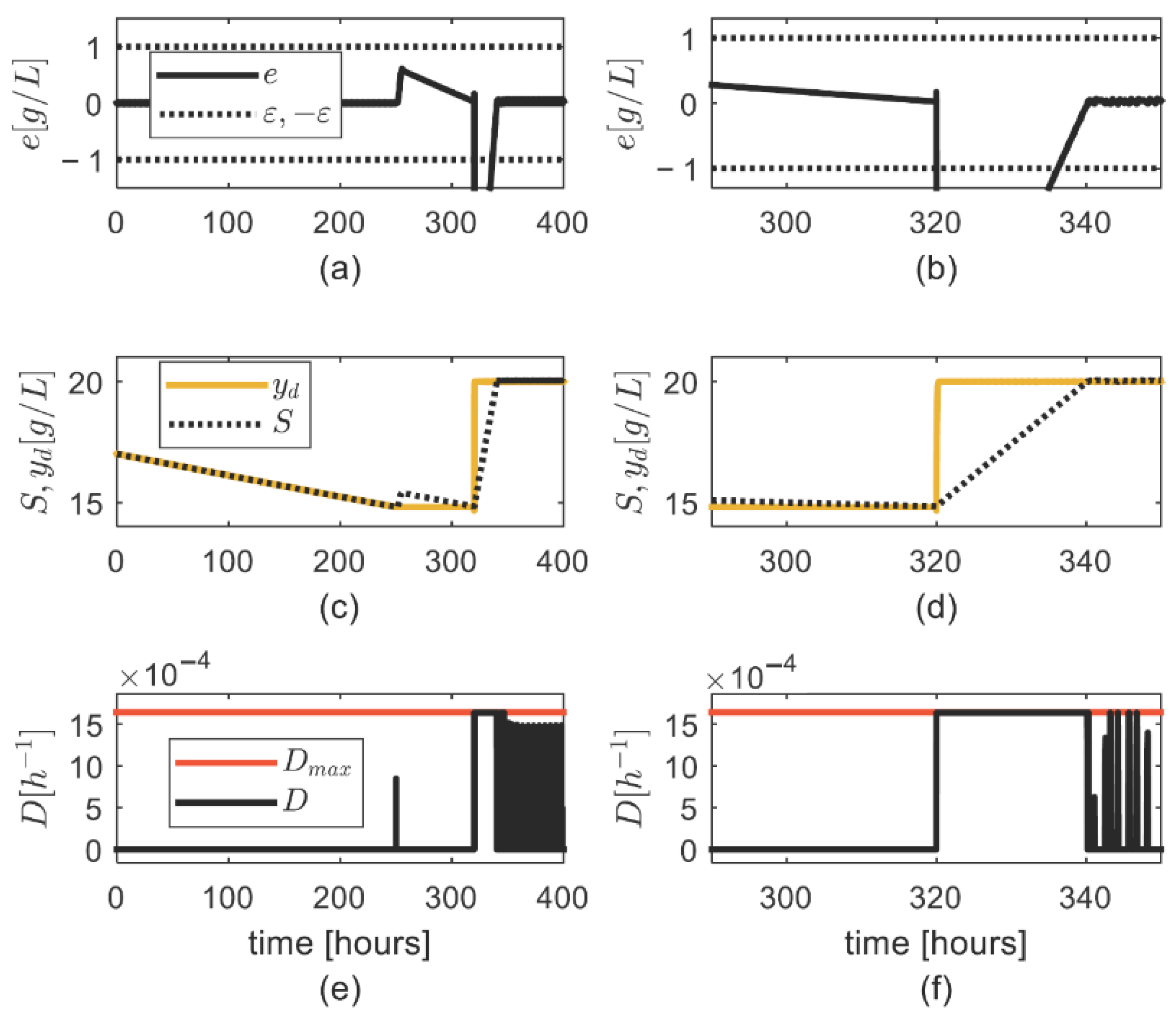
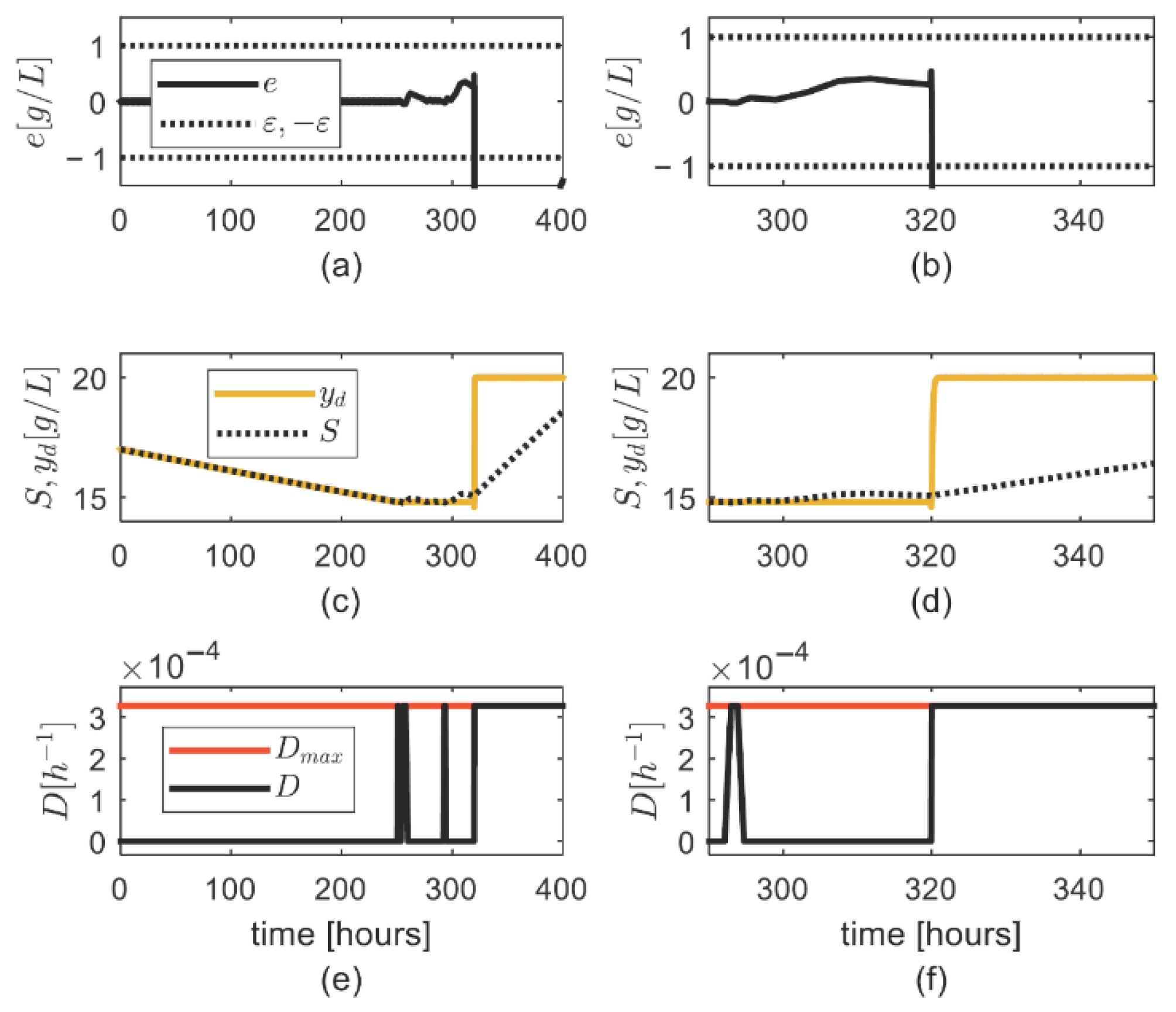
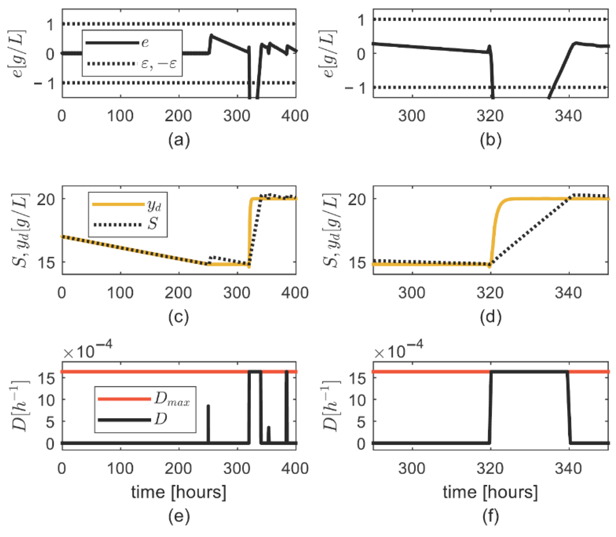
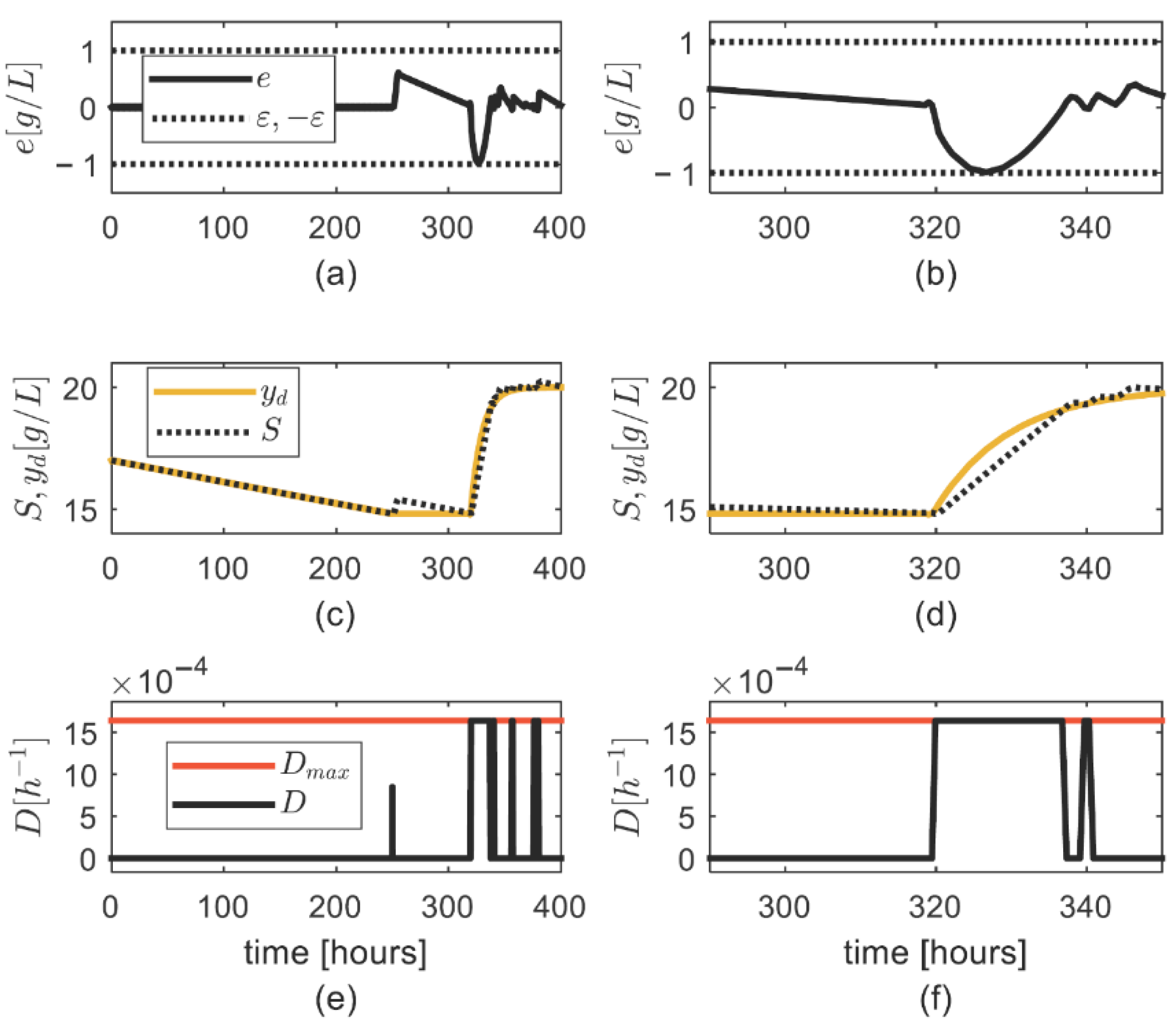
4. Numerical Simulation

In this section, the controller and convergence results stated in Theorem 1 are illustrated through simulation, using bioreactor model (1) subject to Assumptions 1 to 3, the reference model (3), and the controller (4)–(11). We considered the continuous cultivation of Gluconacetobacter diazotrophicus, whose conditions are those of the batch culture described in [37], including initial medium composition, temperature, pH, dissolved oxygen concentration, mixing conditions. The specific growth rate expression is:

$$\mu ={\mu }_{max}{\left(1-\frac{X}{X_{max}}\right)}^f$$

and the parameters of model (1) are fitted to the measurements provided in [37]:

${\mu }_{max}=0.01484$ h⁻¹; $X_{max}=0.32$ g/L; $f=1.607$; $y_s=0.0234$; $m_s=0.22425$ h⁻¹; $x_{to}=0.09$ g/L; $s_{to}=49.6$ g/L; $D=0.005$ h⁻¹. However, the value $s_{in}=53$ g/L was used in controller simulations. The width of the convergence set was chosen to be $\epsilon =1$, and the controller parameters were chosen as follows:

$$\begin{gathered} r_{sk}=0.01; {\phi }_{drd}=1 \\ {k}_1=60;{\gamma }_{\theta }=0.1;k_i=0.1 \end{gathered}$$

The values of $D_{max}$ and $a_m$ were defined according to the simulation cases, defined in

Table 1. Values of $D_{max}$ and $a_m$, for each simulation case.

Simulation Case	${\mathit{D}}_{\mathit{m}\mathit{a}\mathit{x}}\mathbf{Value}$	${\mathit{a}}_{\mathit{m}}\mathbf{Value}$
Case 1	0.0016	20
Case 2	0.0016	0.1
Case 3	0.000327	7
Case 4	0.0016	1

. The $D_{max}$value for each simulation case satisfied condition (6).

As can be deduced from controller (4)–(11), $k_1$ determined the sensitivity of the control signal $D_{cr}$ to the tracking error $e$ according to Equation (4); ${\gamma }_{\theta }$ determined the increase rate of the updated parameter $\widehat{\theta }$, according to Equation (5); $k_i$determined the value of the $W$ signal (7), which, in turn, affected the increase rate of $\widehat{\theta }$, according to Equation (5). The exact values of controller parameters $k_1$, ${\gamma }_{\theta }$, $k_i$, were chosen in accordance with these criteria, and by using some trial and error effort, which is common in adaptive control design based on the Lyapunov function.

Simulations (Figure 3) show that: (i) the tracking error $e$ was inside the residual set ${\mathsf{\Omega }}_e=\left\{e:\left|e\right|\le \epsilon \right\}$ at the initial time, and it is outside ($e<-\epsilon$) for $t\in \left[320336\right]$ h, which was related to the steep increase in the desired output $y_d$ (Figure 3a–d); (ii) there was an saturation event ($D=D_{max}$) associated with the decrease in the tracking error (Figure 3e,f).

Simulations (Figure 4) showed that: (i) the tracking error $e$ was inside the residual set ${\mathsf{\Omega }}_e=\left\{e:\left|e\right|\le \epsilon \right\}$ at the initial time, and remained inside (Figure 4a,b); (ii) there was an upper saturation event for $t\in \left[320 337\right]$ h, featuring $e<0$ and $D=D_{max}$ (Figure 4b,f). Few upper saturation events occurred afterward.

Simulations (Figure 5) show that: (i) the tracking error $e$ is inside the residual set ${\mathsf{\Omega }}_e=\left\{e:\left|e\right|\le \epsilon \right\}$ at initial time, and it is below ($e<-\epsilon$) for $t\in \left[320 400\right]$ h (Figure 5a,b), what is related to a steep increase in the desired output $y_d$, see Figure 5c,d; (ii) there is a sustained upper saturation event ($D=D_{max}$) related to the decrease in $e$ (Figure 5a,b,e,f).

Simulations (Figure 6) show that: (i) the tracking error $e$ is inside the residual set ${\mathsf{\Omega }}_e=\left\{e:\left|e\right|\le \epsilon \right\}$ at initial time, and it is below for $t\in \left[320 336\right]$ h (Figure 6a,b), what is related to the steep increase in the desired output $y_d$ (Figure 6c,d); (ii) there is a sustained upper saturation event ($D=D_{max}$) related to the decrease in the tracking error ($e<-\epsilon$) (Figure 6a,b,e,f).

General Discussion on the Simulation Results

In summary, the simulations showed the performance of controller (4)–(11), with updated parameter $\widehat{\theta }$ provided by Equation (5), considering: (i) the system (1) subject to input saturation condition (2) with $D_{max}$ value fulfilling condition (6) and shown in Figure 3e, Figure 4e, Figure 5e and Figure 6e; (ii) desired output $y_d$ given by reference model (3), featuring time varying but settling behavior and high $d{y}_d/dt$ values during some time lapses, see Figure 3c, Figure 4c, Figure 5c and Figure 6c. It can be noticed that asymptotic convergence of the tracking error $e$ to the compact set ${\mathsf{\Omega }}_e=\left\{e:\left|e\right|\le \epsilon \right\}$ and boundedness of updated parameter $\widehat{\theta }$ were achieved, despite input saturation events, see Figure 3a, Figure 4a, Figure 5a and Figure 6a. The main features of the simulations related to Contributions stated in Introduction were:

−

Asymptotic convergence of the tracking error was achieved during input saturation events (see Figure 3d,f, Figure 4d,f and Figure 6d,f), during time lapses with repeated input saturation events (see Figure 4e,c) and during time lapses featuring high $d{y}_d/dt$ values.

−

Condition (6) for computing $D_{max}$ was adequate, as the asymptotic convergence of the tracking error was achieved.

Other features were:

−

There was no excessive increase in the updated parameter $\widehat{\theta }$, which was also noticed during high $d{y}_d/dt$ values,

−

A fast convergence of the tracking error was achieved by properly setting the controller parameters,

−

The uncertainty on the substrate consumption rate $y_s\mu X$ was properly tackled by means of the updated parameter $\widehat{\theta }$;

−

The uncertainty on $s_{in}$ was properly tackled through the robustness strategy.

During no input saturation events, $D=D_{cr}$ given by Equation (4), and the asymptotic convergence of the tracking error and the control effort corresponded to the case that the adaptive controller was designed for the system with no saturation. During input saturation events, the control input $D$ took on two values, $D\in \left\{D_{min},D_{max}\right\}, D_{min}=0$, and the convergence rate of the tracking error depended on the $D_{max}$ value, model terms, and $d{y}_d/dt$. During a single input saturation event, $D$ remained constant, either $D=D_{min}$ or $D=D_{max}$, so that the system behavior was a case of open loop and the convergence of the tracking error may be slow, see for instance Figure 6d,f.

During the time lapses with large $d{y}_d/dt$ values, a high control effort was required in order to achieve the convergence of the output $y$ to $y_d$. However, the limitation of the control effort through input saturation led to a limited speed of output convergence, so that the tracking error remained outside the target compact set ${\mathsf{\Omega }}_e$ during those time lapses.

In Figure 4c and Figure 6c there was a steep variation in $y$ and $y_d$. The variation rate of $y_d$ was determined by the $a_m$ value, which was noted from the reference model (3); recall that the $a_m$ values are given in Table 1. The high variation rate of $y$ occurred during a time-lapse of fast $y_d$ variation, that is, high $d{y}_d/dt$ values. The fast $y_d$ variation led to a higher tracking error $e$, thus leading to larger control signals $D_{cr}$and $D$, and consequently, a faster change in the output $y$. In summary, a fast change in $y_d$ implies a fast change in $y$, which is related to the control action to achieve convergence of the tracking error. The physical meaning of this steep variation is that a fast change in the desired output $y_d$ implies a fast change in the measured output $y$, which is caused by the response of the actuator to the tracking error signal.

5. Conclusions

In this work, a controller was developed for a continuous bioreactor subject to input saturation, and the convergence of the tracking error and the boundedness of the updated parameter were determined, considering the input saturation events. The substrate concentration and the dilution rate were chosen as output and input, respectively. The asymptotic convergence of the tracking error during input saturation events was determined as a function of the terms and parameters of the reference and system models. The main contributions over closely related works are:

−

Contribution Ci. The effect of input constraint limits and desired output on the convergence of the tracking error during input saturation events was determined.

−

Contribution Cii. The upper limit of the input constraint guaranteeing output convergence during input saturation events was defined as a function of the model terms, but was independent of the time derivative of the desired output and its limit.

−

Contribution Ciii. A new dead zone Lyapunov function was proposed which allows proving the convergence of the tracking error during input saturation events, considering fast variation in the desired output.

The main limitations of the work are: (i) systems in strict feedback nonlinear form of second order and general order were not considered; (ii) the lack of knowledge on the upper and lower bounds of $\left(S_{in}-S\right)$ was not considered; (iii) the presence of time-varying delay caused by reaction time of sensor and actuators, and signal sampling and transmission was not considered; (iv) finite time control strategy and power type reaching law were not considered.

References

1. Alshammari, O.; Mahyuddin, M.N.; Jerbi, H. A Survey on Control Techniques of a Benchmarked Continuous Stirred Tank Reactor. J. Eng. Sci. Technol. 2018, 13, 3277–3296. [Google Scholar]
2. Franco-de los Reyes, H.A.; Alvarez, J. Saturated Output-Feedback Control and State Estimation of a Class of Exothermic Tubular Reactors. J. Process Control 2022, 112, 78–95. [Google Scholar] [CrossRef]
3. Bastin, G.; Dochain, D. On-Line Estimation and Adaptive Control of Bioreactors; Elsevier: Amsterdam, The Netherlands, 1990. [Google Scholar]
4. Méndez-Acosta, H.O.; Campos-Delgado, D.U.; Femat, R.; González-Alvarez, V. A Robust Feedforward/Feedback Control for an Anaerobic Digester. Comput. Chem. Eng. 2005, 29, 1613–1623. [Google Scholar] [CrossRef]
5. Méndez-Acosta, H.O.; Palacios-Ruiz, B.; Alcaraz-González, V.; González-Álvarez, V.; García-Sandoval, J.P. A Robust Control Scheme to Improve the Stability of Anaerobic Digestion Processes. J. Process Control 2010, 20, 375–383. [Google Scholar] [CrossRef]
6. Hägglund, T.; Shinde, S.; Theorin, A.; Thomsen, U. An Industrial Control Loop Decoupler for Process Control Applications. Control Eng. Pract. 2022, 123, 105138. [Google Scholar] [CrossRef]
7. Zhou, Z.; Tang, G.; Huang, H.; Han, L.; Xu, R. Adaptive Nonsingular Fast Terminal Sliding Mode Control for Underwater Manipulator Robotics with Asymmetric Saturation Actuators. Control Theory Technol. 2020, 18, 81–91. [Google Scholar] [CrossRef]
8. Shahriari-Kahkeshi, M. Dead-Zone Model-Based Adaptive Fuzzy Wavelet Control for Nonlinear Systems Including Input Saturation and Dynamic Uncertainties. Int. J. Fuzzy Syst. 2018, 20, 2577–2592. [Google Scholar] [CrossRef]
9. Polycarpou, M.; Farrell, J.; Sharma, M. On-Line Approximation Control of Uncertain Nonlinear Systems: Issues with Control Input Saturation. In Proceedings of the 2003 American Control Conference, Denver, CO, USA, 4–6 June 2003; pp. 543–548. [Google Scholar]
10. Zhang, W.; Yi, W. Fuzzy Observer-Based Dynamic Surface Control for Input-Saturated Nonlinear Systems and Its Application to Missile Guidance. IEEE Access 2020, 8, 121285–121298. [Google Scholar] [CrossRef]
11. Shao, K.; Tang, R.; Xu, F.; Wang, X.; Zheng, J. Adaptive Sliding Mode Control for Uncertain Euler–Lagrange Systems with Input Saturation. J. Frankl. Inst. 2021, 358, 8356–8376. [Google Scholar] [CrossRef]
12. Gao, S.; Ning, B.; Dong, H. Fuzzy Dynamic Surface Control for Uncertain Nonlinear Systems under Input Saturation via Truncated Adaptation Approach. Fuzzy Sets Syst. 2016, 290, 100–117. [Google Scholar] [CrossRef]
13. Min, H.; Xu, S.; Ma, Q.; Zhang, B.; Zhang, Z. Composite-Observer-Based Output-Feedback Control for Nonlinear Time-Delay Systems with Input Saturation and Its Application. IEEE Trans. Ind. Electron. 2018, 65, 5856–5863. [Google Scholar] [CrossRef]
14. Zeinali, S.; Shahrokhi, M. Observer-Based Singularity Free Nonlinear Controller for Uncertain Systems Subject to Input Saturation. Eur. J. Control 2020, 52, 49–58. [Google Scholar] [CrossRef]
15. Meng, R.; Chen, S.; Hua, C.; Qian, J.; Sun, J. Disturbance Observer-Based Output Feedback Control for Uncertain QUAVs with Input Saturation. Neurocomputing 2020, 413, 96–106. [Google Scholar] [CrossRef]
16. Wang, F.; Zhou, C.; Wang, J.; Hua, C. Adaptive Fuzzy Output Feedback Controller Design for a HAGC System with Input Saturation and Output Error Constraints. J. Frankl. Inst. 2022, 359, 2030–2057. [Google Scholar] [CrossRef]
17. Li, H.; Liu, Q.; Kong, L.; Zhang, X. Design of Adaptive Tracking Controller Using Barrier Functions for Nonlinear Systems with Input Saturation. J. Frankl. Inst. 2020, 357, 12555–12570. [Google Scholar] [CrossRef]
18. Sun, J.; Liu, C. Auxiliary-System-Based Composite Adaptive Optimal Backstepping Control for Uncertain Nonlinear Guidance Systems with Input Constraints. ISA Trans. 2020, 107, 294–306. [Google Scholar] [CrossRef]
19. Askari, M.R.; Shahrokhi, M.; Khajeh Talkhoncheh, M. Observer-Based Adaptive Fuzzy Controller for Nonlinear Systems with Unknown Control Directions and Input Saturation. Fuzzy Sets Syst. 2017, 314, 24–45. [Google Scholar] [CrossRef]
20. Golkani, M.A.; Seeber, R.; Reichhartinger, M.; Horn, M. Lyapunov-based Saturated Continuous Twisting Algorithm. Int. J. Robust Nonlinear Control 2021, 31, 3513–3527. [Google Scholar] [CrossRef]
21. Dochain, D.; Perrier, M.; Guay, M. Extremum Seeking Control and Its Application to Process and Reaction Systems: A Survey. Math. Comput. Simul. 2011, 82, 369–380. [Google Scholar] [CrossRef]
22. de Battista, H.; Jamilis, M.; Garelli, F.; Picó, J. Global Stabilisation of Continuous Bioreactors: Tools for Analysis and Design of Feeding Laws. Automatica 2018, 89, 340–348. [Google Scholar] [CrossRef]
23. Picó, J.; de Battista, H.; Garelli, F. Smooth Sliding-Mode Observers for Specific Growth Rate and Substrate from Biomass Measurement. J. Process Control 2009, 19, 1314–1323. [Google Scholar] [CrossRef]
24. Neria-González, M.I.; Domínguez-Bocanegra, A.R.; Torres, J.; Maya-Yescas, R.; Aguilar-López, R. Linearizing Control Based on Adaptive Observer for Anaerobic Sulphate Reducing Bioreactors with Unknown Kinetics. Chem. Biochem. Eng. Q. 2009, 23, 179–185. [Google Scholar]
25. Slotine, J.-J.; Li, W. Applied Nonlinear Control; Prentice Hall: Englewood Cliffs, NJ, USA, 1991. [Google Scholar]
26. Astrom, K.J.; Wittenmark, B. Adaptive Control; Addison-Wesley Publishing Company: Reading, MA, USA, 1995. [Google Scholar]
27. Koo, K.-M. Stable Adaptive Fuzzy Controller with Time-Varying Dead-Zone. Fuzzy Sets Syst. 2001, 121, 161–168. [Google Scholar] [CrossRef]
28. Wang, X.-S.; Su, C.-Y.; Hong, H. Robust Adaptive Control of a Class of Nonlinear Systems with Unknown Dead-Zone. Automatica 2004, 40, 407–413. [Google Scholar] [CrossRef]
29. Ranjbar, E.; Yaghubi, M.; Abolfazl Suratgar, A. Robust Adaptive Sliding Mode Control of a MEMS Tunable Capacitor Based on Dead-Zone Method. Automatika 2020, 61, 587–601. [Google Scholar] [CrossRef]
30. Hong, Q.; Shi, Y.; Chen, Z. Dynamics Modeling and Tension Control of Composites Winding System Based on ASMC. IEEE Access 2020, 8, 102795–102810. [Google Scholar] [CrossRef]
31. Rincón, A.; Hoyos, F.E.; Candelo-Becerra, J.E. Adaptive Control for a Biological Process under Input Saturation and Unknown Control Gain via Dead Zone Lyapunov Functions. Appl. Sci. 2020, 11, 251. [Google Scholar] [CrossRef]
32. Rincón, A.; Restrepo, G.M.; Hoyos, F.E. A Robust Observer—Based Adaptive Control of Second—Order Systems with Input Saturation via Dead-Zone Lyapunov Functions. Computation 2021, 9, 82. [Google Scholar] [CrossRef]
33. Rincón, A.; Restrepo, G.M.; Sánchez, Ó.J. An Improved Robust Adaptive Controller for a Fed-Batch Bioreactor with Input Saturation and Unknown Varying Control Gain via Dead-Zone Quadratic Forms. Computation 2021, 9, 100. [Google Scholar] [CrossRef]
34. Ioannou, P.A.; Sun, J. Robust Adaptive Control; Prentice-Hall PTR: Upper Saddle River, NJ, USA, 1996. [Google Scholar]
35. Liu, C.; Yue, X.; Zhang, J.; Shi, K. Active Disturbance Rejection Control for Delayed Electromagnetic Docking of Spacecraft in Elliptical Orbits. IEEE Trans. Aerosp. Electron. Syst. 2021, 58, 2257–2268. [Google Scholar] [CrossRef]
36. Shi, K.; Liu, C.; Sun, Z.; Yue, X. Coupled Orbit-Attitude Dynamics and Trajectory Tracking Control for Spacecraft Electromagnetic Docking. Appl. Math. Model. 2022, 101, 553–572. [Google Scholar] [CrossRef]
37. Rincón, A.; Cuellar, J.A.; Valencia, L.F.; Sánchez, O.J. Cinética de Crecimiento de Gluconacetobacter Diazotrophicus Usando Melaza de Caña y Sacarosa: Evaluación de Modelos Cinéticos. Acta Biol. Colomb. 2019, 24, 38–57. [Google Scholar] [CrossRef]
Figure 1. Overall steps of the controller design and stability analysis.
Symmetry 14 01232 g001
Figure 2. Block diagram of the proposed controller.
Symmetry 14 01232 g002
Figure 3. Simulation results for case 1: (a) Trajectory of the tracking error e ; (b) detail of the trajectory of e ; (c) trajectory of substrate concentration S ; (d) detail of the trajectory of S ; (e) trajectory of the control input D ; (f) detail of the trajectory of D .
Symmetry 14 01232 g003
Figure 4. Simulation results for case 2: (a) Trajectory of the tracking error e ; (b) detail of the trajectory of e ; (c) trajectory of substrate concentration S ; (d) detail of the trajectory of S ; (e) trajectory of the control input D ; (f) detail of the trajectory of D .
Symmetry 14 01232 g004
Figure 5. Simulation results for case 3: (a) Trajectory of the tracking error e ; (b) detail of the trajectory of e ; (c) trajectory of substrate concentration S ; (d) detail of the trajectory of S ; (e) trajectory of the control input D ; (f) detail of the trajectory of D .
Symmetry 14 01232 g005
Figure 6. Simulation results for case 4: (a) Trajectory of the tracking error e ; (b) detail of the trajectory of e ; (c) trajectory of substrate concentration S ; (d) detail of the trajectory of S ; (e) trajectory of the control input D ; (f) detail of the trajectory of D .
Symmetry 14 01232 g006