Figure 1.
Incorrect (a,b) and correct wire intersections (c,d).
Figure 1.
Incorrect (a,b) and correct wire intersections (c,d).
Figure 2.
Incorrect (a) and correct (b) setting of the excitation source at the wire intersection.
Figure 2.
Incorrect (a) and correct (b) setting of the excitation source at the wire intersection.
Figure 3.
A wire-gird element (a) and the area of one wire surface (b).
Figure 3.
A wire-gird element (a) and the area of one wire surface (b).
Figure 4.
Modeling a curved surface with a single wire.
Figure 4.
Modeling a curved surface with a single wire.
Figure 5.
The workflow of the developed module (wire-grid).
Figure 5.
The workflow of the developed module (wire-grid).
Figure 6.
Demonstration of the equal area rule [
28] (
a) and its modification (
b).
Figure 6.
Demonstration of the equal area rule [
28] (
a) and its modification (
b).
Figure 7.
The RP of a dipole on a conducting plate modeled using the wire-grid by (1) (a), by (3) (b), and EMPro (c).
Figure 7.
The RP of a dipole on a conducting plate modeled using the wire-grid by (1) (a), by (3) (b), and EMPro (c).
Figure 8.
The RP of a dipole on a conducting plate at θ = 0, 1, …, 180°, φ = 0° (a), 45° (b), and 90° (c) using the wire-grid by (1) (––), by (3) (----), and EMPro (····).
Figure 8.
The RP of a dipole on a conducting plate at θ = 0, 1, …, 180°, φ = 0° (a), 45° (b), and 90° (c) using the wire-grid by (1) (––), by (3) (----), and EMPro (····).
Figure 9.
The conical (a) and the biconical (b) AEs.
Figure 9.
The conical (a) and the biconical (b) AEs.
Figure 10.
A general view of the biconical AE at frequencies of 0.1 (a), 0.5 (b), and 1 GHz (c) (the view is changing because the wire radius reduces with the frequency growth).
Figure 10.
A general view of the biconical AE at frequencies of 0.1 (a), 0.5 (b), and 1 GHz (c) (the view is changing because the wire radius reduces with the frequency growth).
Figure 11.
The normalized RP (|E|N, times) of the biconical AE with a = 508 mm and Θ1 = Θ2 = 53.1° when ka1 = 1.0640 (f1 = 0.1 GHz), calculated by the wire-grid and EMPro.
Figure 11.
The normalized RP (|E|N, times) of the biconical AE with a = 508 mm and Θ1 = Θ2 = 53.1° when ka1 = 1.0640 (f1 = 0.1 GHz), calculated by the wire-grid and EMPro.
Figure 12.
The normalized RP (|E|N, times) of the biconical AE with a = 508 mm and Θ1 = Θ2 = 53.1° when ka2 = 5.3198 (f1 = 0.5 GHz), calculated by the wire-grid and EMPro.
Figure 12.
The normalized RP (|E|N, times) of the biconical AE with a = 508 mm and Θ1 = Θ2 = 53.1° when ka2 = 5.3198 (f1 = 0.5 GHz), calculated by the wire-grid and EMPro.
Figure 13.
The normalized RP (|E|N, times) of the biconical AE with a = 508 mm and Θ1 = Θ2 = 53.1° when ka3 = 10.6395 (f1 = 1 GHz), calculated by the wire-grid and EMPro.
Figure 13.
The normalized RP (|E|N, times) of the biconical AE with a = 508 mm and Θ1 = Θ2 = 53.1° when ka3 = 10.6395 (f1 = 1 GHz), calculated by the wire-grid and EMPro.
Figure 14.
The normalized RP (|
E|
N, times) of the biconical AE when
ka1 = 1.0640 (
f1 = 0.1 GHz), calculated analytically [
61] and by the wire-grid and EMPro at different mesh sizes.
Figure 14.
The normalized RP (|
E|
N, times) of the biconical AE when
ka1 = 1.0640 (
f1 = 0.1 GHz), calculated analytically [
61] and by the wire-grid and EMPro at different mesh sizes.
Figure 15.
The normalized RP (|
E|
N, times) of the biconical AE when
ka2 = 5.3198 (
f1 = 0.5 GHz), calculated analytically [
61] and by the wire-grid and EMPro at different mesh sizes.
Figure 15.
The normalized RP (|
E|
N, times) of the biconical AE when
ka2 = 5.3198 (
f1 = 0.5 GHz), calculated analytically [
61] and by the wire-grid and EMPro at different mesh sizes.
Figure 16.
The normalized RP (|
E|
N, times) of the biconical AE when
ka3 = 10.6395 (
f1 = 1 GHz), calculated analytically [
61] and by the wire-grid and EMPro at different mesh sizes.
Figure 16.
The normalized RP (|
E|
N, times) of the biconical AE when
ka3 = 10.6395 (
f1 = 1 GHz), calculated analytically [
61] and by the wire-grid and EMPro at different mesh sizes.
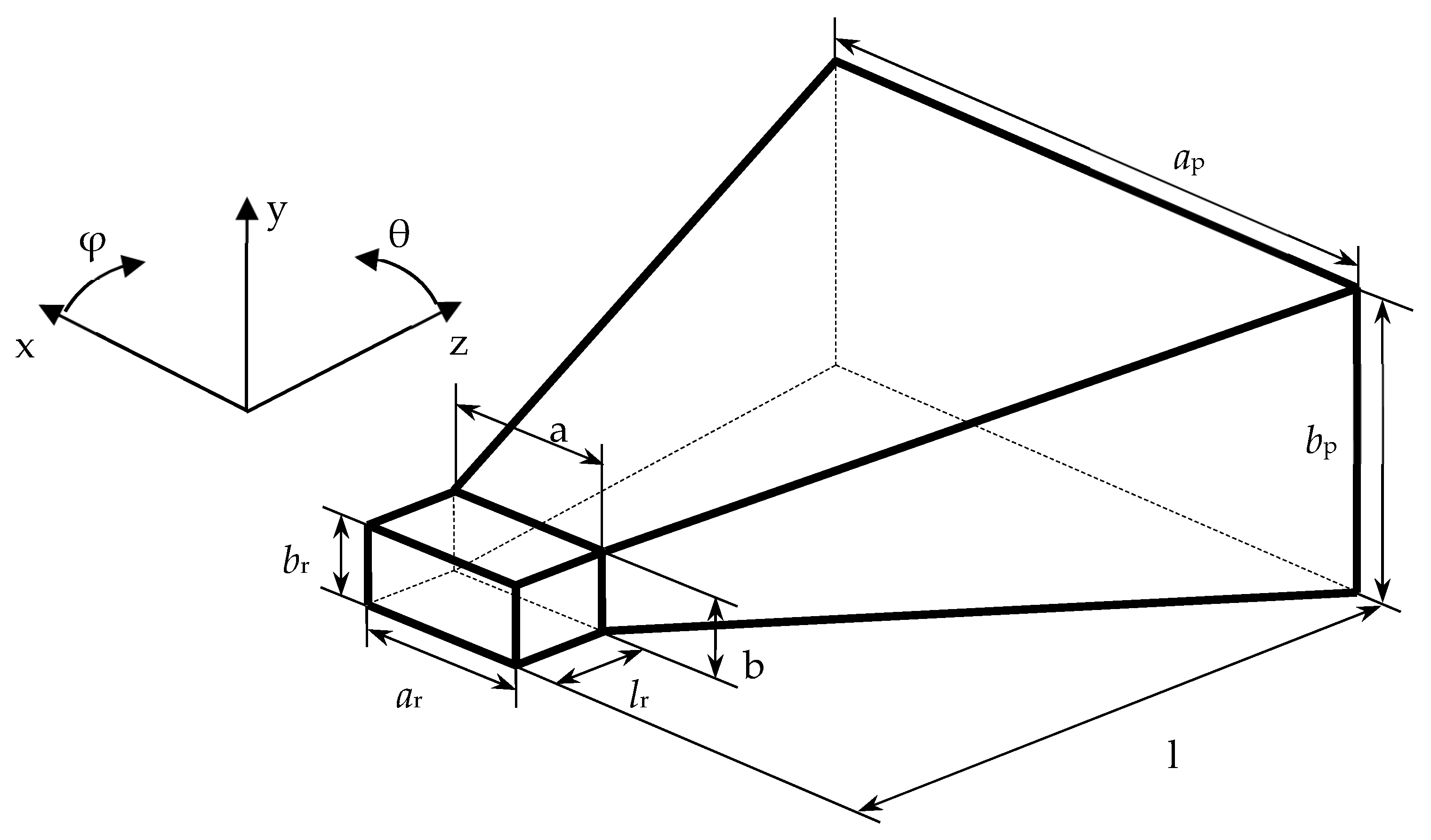
Figure 17.
The isometric view of the inner surface of the horn AE.
Figure 17.
The isometric view of the inner surface of the horn AE.
Figure 18.
General views of AEs with the wire used as an excitation source built in the wire-grid using Le = 16 and Lr = 2 (a), 4 (b), 8 (c), and 16 (d).
Figure 18.
General views of AEs with the wire used as an excitation source built in the wire-grid using Le = 16 and Lr = 2 (a), 4 (b), 8 (c), and 16 (d).
Figure 19.
The RPs (|E|N, dB) of the horn AE at the frequency of 8 GHz in the φ = 90° (a) and φ = 0° (b) planes in the wire-grid with Le = 16 and Lr = 8, n = 10, 20, 40.
Figure 19.
The RPs (|E|N, dB) of the horn AE at the frequency of 8 GHz in the φ = 90° (a) and φ = 0° (b) planes in the wire-grid with Le = 16 and Lr = 8, n = 10, 20, 40.
Figure 20.
The measured (—) and the calculated (····) RPs (|E|N, dB) of the horn AE at the frequency of 8 GHz in the φ = 90° (a) and φ = 0° (b) planes in the wire-grid with Le = 16 and Lr = 8, n = 40. The level of −3 dB (---).
Figure 20.
The measured (—) and the calculated (····) RPs (|E|N, dB) of the horn AE at the frequency of 8 GHz in the φ = 90° (a) and φ = 0° (b) planes in the wire-grid with Le = 16 and Lr = 8, n = 40. The level of −3 dB (---).
Figure 21.
The measured and the calculated RPs (|E|N, dB) of the horn AE at the frequency of 8 GHz in the φ = 90° (a) and φ = 0° (b) planes in the wire-grid with Lr = 8, n = 40, Le = 16, 32, and SZe = SXe or equal to SXe*2±1. The level of −3 dB (---).
Figure 21.
The measured and the calculated RPs (|E|N, dB) of the horn AE at the frequency of 8 GHz in the φ = 90° (a) and φ = 0° (b) planes in the wire-grid with Lr = 8, n = 40, Le = 16, 32, and SZe = SXe or equal to SXe*2±1. The level of −3 dB (---).
Figure 22.
The measured and the calculated RPs (|E|N, dB) of the horn AE at the frequency of 8 GHz in the φ = 90° (a) and φ = 0° (b) planes in the wire-grid with Lr = 16, n = 40, Le = 16, 32, and SZe = SXe or equal to SXe*2±1. The level of −3 dB (---).
Figure 22.
The measured and the calculated RPs (|E|N, dB) of the horn AE at the frequency of 8 GHz in the φ = 90° (a) and φ = 0° (b) planes in the wire-grid with Lr = 16, n = 40, Le = 16, 32, and SZe = SXe or equal to SXe*2±1. The level of −3 dB (---).
Figure 23.
The measured and the calculated RPs (|E|N, dB) of the horn AE at the frequency of 8 GHz in the φ = 90° (a) and φ = 0° (b) planes in the wire-grid with Lr = 32, n = 40, Le = 16, 32, and SZe = SXe or equal to SXe*2±1. The level of −3 dB (---).
Figure 23.
The measured and the calculated RPs (|E|N, dB) of the horn AE at the frequency of 8 GHz in the φ = 90° (a) and φ = 0° (b) planes in the wire-grid with Lr = 32, n = 40, Le = 16, 32, and SZe = SXe or equal to SXe*2±1. The level of −3 dB (---).
Figure 24.
The measured and the calculated RPs (|E|N, dB) of the horn AE at the frequency of 8 GHz in the φ = 90° (a) and φ = 0° (b) planes in the wire-grid with Lr = 8, 16, 32, n = 40, Le = 16, 32, and SZe = SXe or equal to SXe*2±1. The level of −3 dB (---).
Figure 24.
The measured and the calculated RPs (|E|N, dB) of the horn AE at the frequency of 8 GHz in the φ = 90° (a) and φ = 0° (b) planes in the wire-grid with Lr = 8, 16, 32, n = 40, Le = 16, 32, and SZe = SXe or equal to SXe*2±1. The level of −3 dB (---).
Figure 25.
The measured and the calculated RPs (|E|N, dB) of the horn AE at the frequency of 8 GHz in the φ = 90° (a) and φ = 0° (b) planes in the wire-grid with Lr = 8, 16, 32, n = 40, Le = 32, and SZe = SXe. The level of −3 dB (---).
Figure 25.
The measured and the calculated RPs (|E|N, dB) of the horn AE at the frequency of 8 GHz in the φ = 90° (a) and φ = 0° (b) planes in the wire-grid with Lr = 8, 16, 32, n = 40, Le = 32, and SZe = SXe. The level of −3 dB (---).
Table 1.
The matrix Z orders N and their condition numbers, for the biconical AE with a = 508 mm and Θ1 = Θ2 = 53.1° at frequencies of 0.1, 0.2, and 1 GHz and mesh step (segment size) λ/n.
Table 1.
The matrix Z orders N and their condition numbers, for the biconical AE with a = 508 mm and Θ1 = Θ2 = 53.1° at frequencies of 0.1, 0.2, and 1 GHz and mesh step (segment size) λ/n.
| Frequency (GHz) | n | N | cond(Z) |
|---|
| 0.1 | 10 | 257 | 1.4 × 10⁵ |
| 20 | 513 | 2.2 × 10⁶ |
| 40 | 897 | 3.1 × 10⁵ |
| 0.5 | 10 | 1153 | 2.7 × 10⁵ |
| 20 | 2177 | 5.7 × 10⁵ |
| 40 | 4353 | 9.6 × 10⁶ |
| 1 | 10 | 2177 | 8.2 × 10⁴ |
| 20 | 4353 | 1.6 × 10⁵ |
| 40 | 8705 | 6.4 × 10⁵ |
Table 2.
The input impedance values for the biconical AE with a = 508 mm and Θ1 = Θ2 = 53.1° at frequencies of 0.1, 0.2, and 1 GHz and a mesh step (segment size) λ/n.
Table 2.
The input impedance values for the biconical AE with a = 508 mm and Θ1 = Θ2 = 53.1° at frequencies of 0.1, 0.2, and 1 GHz and a mesh step (segment size) λ/n.
| Frequency (GHz) | n | (A1), (A11) | EMPro | Wire-Grid |
|---|
| 0.1 | 10 | 40.40 + j28.32 | 29.73 + j15.78 | 0.46 − j25.48 |
| 20 | 39.51 + j12.95 | 192.31 − j58.89 |
| 40 | – | 28.01 + j25.59 |
| 0.5 | 10 | 101.80 − j9.38 | 117.48 + j64.27 | 114.01 − j6.29 |
| 20 | 112.89 + j74.69 | 102.02 + j33.36 |
| 40 | – | 90.44 + j48.18 |
| 1 | 10 | 88.64 + j16.68 | 116.40 + j89.92 | 103.11 + j41.34 |
| 20 | 117.84 + j112.36 | 88.29 + j56.82 |
| 40 | – | 84.62 + j71.55 |
Table 3.
The deviation (%) of the input impedance magnitudes from
Table 2 calculated using the wire-grid and EMPro compared to those obtained analytically.
Table 3.
The deviation (%) of the input impedance magnitudes from
Table 2 calculated using the wire-grid and EMPro compared to those obtained analytically.
| Frequency (GHz) | n | EMPro | Wire-Grid |
|---|
| 0.1 | 10 | 31.78 | 48.35 |
| 20 | 15.73 | 307.65 |
| 40 | – | 23.10 |
| 0.5 | 10 | 30.99 | 11.69 |
| 20 | 32.41 | 4.99 |
| 40 | – | 0.23 |
| 1 | 10 | 63.08 | 23.16 |
| 20 | 80.52 | 16.41 |
| 40 | – | 22.86 |
Table 4.
The elapsed time and used memory for simulating the biconical AE using the wire-grid, with a = 508 mm and Θ1 = Θ2 = 53.1° at frequencies of 0.1, 0.2, and 1 GHz and a mesh step (segment size) λ/n.
Table 4.
The elapsed time and used memory for simulating the biconical AE using the wire-grid, with a = 508 mm and Θ1 = Θ2 = 53.1° at frequencies of 0.1, 0.2, and 1 GHz and a mesh step (segment size) λ/n.
| Frequency (GHz) | n | T (s) | M (MB) |
|---|
| 0.1 | 10 | 0.34 | 1 |
| 20 | 0.51 | 4 |
| 40 | 0.60 | 12.28 |
| 0.5 | 10 | 1.02 | 20.29 |
| 20 | 4.11 | 72.31 |
| 40 | 19.29 | 289.13 |
| 1 | 10 | 4.03 | 72.31 |
| 20 | 18.29 | 289.13 |
| 40 | 109.06 | 1156.27 |
Table 5.
The elapsed time to obtain the RTC at each frequency, the total simulation time (Tt), and the used memory for simulating the biconical AE using EMPro with a = 508 mm and Θ1 = Θ2 = 53.1° at frequencies of 0.1, 0.2, and 1 GHz and a mesh step (segment size) λ/n.
Table 5.
The elapsed time to obtain the RTC at each frequency, the total simulation time (Tt), and the used memory for simulating the biconical AE using EMPro with a = 508 mm and Θ1 = Θ2 = 53.1° at frequencies of 0.1, 0.2, and 1 GHz and a mesh step (segment size) λ/n.
| n | Frequency (GHz) | T (s) | Tt (s) | Physical/Virtual Memory (MB) | Required (GB) | Problem Size (Cells) |
|---|
| 10 | 0.1 | 159 | 921 | 903/922 | 1.2 | 331 × 311 × 245 |
| 0.5 | 181 |
| 1 | 183 |
| 20 | 0.1 | 567 | 1892 | 4722/4753 | 6 | 584 × 581 × 448 |
| 0.5 | 649 |
| 1 | 676 |
| 40 | 0.1 | – | – | – | 36 | 1126 × 1120 × 855 |
| 0.5 | – | – |
| 1 | – | – |
Table 6.
The maximum differences of normalized RP values obtained at different mesh sizes λ/n and by (A8) at frequencies of 0.1, 0.2, and 1 GHz.
Table 6.
The maximum differences of normalized RP values obtained at different mesh sizes λ/n and by (A8) at frequencies of 0.1, 0.2, and 1 GHz.
| Frequency (GHz) | n | EMPro | Wire-Grid |
|---|
| 0.1 | 10 | 0.0189 | 0.0259 |
| 20 | 0.0189 | 0.0236 |
| 40 | – | 0.0211 |
| 0.5 | 10 | 0.1080 | 0.1869 |
| 20 | 0.1030 | 0.1395 |
| 40 | – | 0.1395 |
| 1 | 10 | 0.1291 | 0.1569 |
| 20 | 0.1268 | 0.1197 |
| 40 | – | 0.1669 |
Table 7.
The geometrical parameters (mm) of the inner surface of the horn AE.
Table 7.
The geometrical parameters (mm) of the inner surface of the horn AE.
| Geometrical Parameter | ap | bp | a | b | ar | br | l | lr |
|---|
| Model | 80 | 60 | 23 | 10 | 23 | 10 | 150 | 10 |
| Prototype | 79.9 | 59.8 | 23.0 | 10.0 | 23.0 | 10.0 | 149.9 | 10.0 |
Table 8.
Total wire number (TWN) and the order N of the SLAE matrix Z for the horn AE at different mesh step of the grid λ/n using the wire-grid and Le = 16, and Lr = 2, 4, 8, 16; the condition number for matrix Z (cond(Z)) and the time consumed to calculate Z (T).
Table 8.
Total wire number (TWN) and the order N of the SLAE matrix Z for the horn AE at different mesh step of the grid λ/n using the wire-grid and Le = 16, and Lr = 2, 4, 8, 16; the condition number for matrix Z (cond(Z)) and the time consumed to calculate Z (T).
| Lr | TWN | n |
|---|
| 10 | 20 | 40 |
|---|
| N | T (s) | cond(Z) | N | T (s) | cond(Z) | N | T (s) | cond(Z) |
|---|
| 2 | 1609 | 3544 | 1.65 | 2.35 × 10⁴ | 5931 | 4.40 | 8.68 × 10⁴ | 11,448 | 16.80 | 3.76 × 10⁵ |
| 4 | 1687 | 3636 | 1.71 | 2.41 × 10⁴ | 6112 | 4.73 | 8.91 × 10⁴ | 11,742 | 17.46 | 1.89 × 10⁶ |
| 8 | 1999 | 3906 | 2.01 | 3.28 × 10⁴ | 6480 | 5.25 | 1.02 × 10⁵ | 12,464 | 19.25 | 4.48 × 10⁵ |
| 16 | 3247 | 5178 | 3.44 | 3.69 × 10⁵ | 7556 | 7.10 | 2.07 × 10⁶ | 13,936 | 24.49 | 9.81 × 10⁵ |
Table 9.
The calculated and measured RTCs of the horn AE.
Table 9.
The calculated and measured RTCs of the horn AE.
| RTC | Wire-Grid | Measured |
|---|
| BW (°), φ = 90° | 25 | 31 |
| BW (°), φ = 0° | 34 | 31 |
| SLmax (dB) | −12.61 | −16.93 |
Table 10.
The calculated RTCs of the horn AE using the wire-grid with different mesh and grid settings.
Table 10.
The calculated RTCs of the horn AE using the wire-grid with different mesh and grid settings.
| | n |
|---|
| | 10 | 20 | 40 |
|---|
| Lr | 8 | 16 | 32 | 8 | 16 | 32 | 8 | 16 | 32 |
|---|
| SXe | 16 | 32 | 16 | 32 | 16 | 32 | 16 | 32 | 16 | 32 | 16 | 32 | 16 | 32 | 16 | 32 | 16 | 32 |
|---|
| SZe | 16 | 32 | 16 | 32 | 16 | 32 | 16 | 32 | 16 | 32 | 16 | 32 | 16 | 32 | 16 | 32 | 16 | 32 | 16 | 32 | 16 | 32 | 16 | 32 | 16 | 32 | 16 | 32 | 16 | 32 | 16 | 32 | 16 | 32 | 16 | 32 |
|---|
| TWN | 1584 + 415 | 3120 + 415 | 3168 + 415 | 6240 + 415 | 1584 + 1663 | 3120 + 1663 | 3168 + 1663 | 6240 + 1663 | 1584 + 6655 | 3120 + 6655 | 3168 + 6655 | 6240 + 6655 | 1584 + 415 | 3120 + 415 | 3168 + 415 | 6240 + 415 | 1584 + 1663 | 3120 + 1663 | 3168 + 1663 | 6240 + 1663 | 1584 + 6655 | 3120 + 6655 | 3168 + 6655 | 6240 + 6655 | 1584 + 415 | 3120 + 415 | 3168 + 415 | 6240 + 415 | 1584 + 1663 | 3120 + 1663 | 3168 + 1663 | 6240 + 1663 | 1584 + 6655 | 3120 + 6655 | 3168 + 6655 | 6240 + 6655 |
| N | 3906 | 5794 | 6674 | 9746 | 5178 | 7066 | 7946 | 11,018 | 10,218 | 12,106 | 12,986 | 16,058 | 6480 | 9120 | 10,688 | 14,464 | 7556 | 10,196 | 11,764 | 15,540 | 12,644 | 15,284 | 16,852 | 20,628 | 12,464 | 15,792 | 20,544 | 24,288 | 13,936 | 17,264 | 22,016 | 25,760 | 18,232 | 21,560 | 26,312 | 30,056 |
| T (s) | 6.42 | 15.12 | 21.60 | 52.72 | 12.43 | 24.05 | 31.47 | 64.34 | 54.28 | 83.22 | 97.87 | 167.24 | 19.10 | 41.30 | 61.06 | 131.29 | 27.56 | 55.39 | 77.57 | 157.34 | 92.08 | 154.39 | 186.79 | 311.35 | 90.19 | 161.69 | 311.84 | 473.22 | 121.86 | 202.88 | 372.68 | 542.52 | 219.29 | 352.75 | 570.93 | 851.60 |
|
cond (Z) | 3.28 × 10⁴ | 5.02 × 10⁴ | 7.37 × 10⁴ | 1.50 × 10⁵ | 3.69 × 10⁵ | 4.50 × 10⁵ | 4.72 × 10⁵ | 6.05 × 10⁵ | 2.75 × 10⁷ | 3.12 × 10⁷ | 5.10 × 10⁷ | 5.91 × 10⁷ | 1.03 × 10⁵ | 1.26 × 10⁵ | 1.80 × 10⁵ | 2.60 × 10⁵ | 2.07 × 10⁶ | 2.49 × 10⁶ | 2.56 × 10⁶ | 3.15 × 10⁶ | 5.28 × 10⁶ | 5.80 × 10⁶ | 5.96 × 10⁶ | 6.77 × 10⁶ | 4.48 × 10⁵ | 4.58 × 10⁵ | 8.76 × 10⁵ | 7.89 × 10⁵ | 9.81 × 10⁵ | 1.07 × 10⁶ | 1.40 × 10⁶ | 1.44 × 10⁶ | 2.94 × 10⁶ | 3.15 × 10⁶ | 3.50 × 10⁶ | 3.72 × 10⁶ |
| R (Ohm) | 227.18 | 298.17 | 231.90 | 303.70 | 217.05 | 287.70 | 224.36 | 290.93 | 217.33 | 287.74 | 222.93 | 289.09 | 215.68 | 274.68 | 226.40 | 293.19 | 205.07 | 264.48 | 216.17 | 279.08 | 204.48 | 263.96 | 2113.53 | 275.19 | 210.86 | 242.17 | 221.74 | 275.12 | 199.63 | 234.12 | 212.97 | 266.42 | 193.60 | 228.65 | 207.58 | 259.63 |
| X (Ohm) | 267.54 | 274.63 | 267.14 | 288.83 | 275.49 | 290.37 | 275.55 | 304.27 | 277.11 | 292.70 | 276.17 | 305.65 | 330.36 | 306.99 | 326.06 | 321.58 | 341.40 | 328.61 | 339.68 | 346.79 | 345.87 | 335.80 | 342.88 | 352.96 | 400.66 | 366.40 | 389.78 | 368.76 | 415.03 | 388.28 | 407.21 | 399.02 | 419.44 | 395.82 | 413.16 | 409.90 |
| |Z| (Ohm) | 349.05 | 405.37 | 353.76 | 419.12 | 350.73 | 408.76 | 355.34 | 420.98 | 352.16 | 410.44 | 354.92 | 167.24 | 394.50 | 411.94 | 396.95 | 435.17 | 398.26 | 421.83 | 402.63 | 445.14 | 401.79 | 427.13 | 403.93 | 447.57 | 452.75 | 439.20 | 448.43 | 460.08 | 460.55 | 453.40 | 459.54 | 479.79 | 461.96 | 457.11 | 462.38 | 485.20 |


 ,
, 


