Abstract
Aiming at the problems of difficult handling of three-dimensional flight conflicts and unfair distribution of resolution costs, we propose a multi-aircraft conflict resolution method based on the network cooperative game. Firstly, we establish a flight conflict network model with aircraft as nodes and the conflict relationship between node pairs as edges. After that, we propose a comprehensive network index that can evaluate the effect of resolution strategy. Based on the concept of “nucleolus solution”, we establish a conflict network alliance with all nodes as participants, and balance the interests of all participants through the resolution cost function. In order to improve the timeliness of the method, we propose two optimization methods: adjusting high-priority nodes and customizing the initial resolution scheme. Finally, we combine the NSGA-II algorithm to solve the optimal conflict resolution scheme. The simulation results show that our method can adjust 10 aircraft in 15.17 s and resolve 12 flight conflicts in a complex conflict scenario containing 40 aircraft; our method reduces the resolution cost by more than 22.1% on average compared with the method without considering the resolution cost. The method ensures both the conflict resolution capability and the reduction in resolution cost.
1. Introduction
In recent years, with the continuous increase in air traffic flow, the contradiction between limited airspace resources and growing shipping demand has become increasingly prominent. The congested airspace leads to an increased possibility of flight conflicts, and flight conflicts are an essential cause of flight accidents. Therefore, effectively avoiding flight conflicts, especially in a complex environment with crowded airspace and a large number of potential flight conflicts, provides controllers with effective and feasible conflict resolution solutions, which has become an urgent problem to be solved.
At present, common conflict resolution methods include: the geometric method, artificial potential field method, swarm intelligence algorithm, optimal control method, game theory, complex network method, etc. Durand et al. apply the velocity obstacle method in the field of robot obstacle avoidance to the study of aircraft collision avoidance, and derives an optimal obstacle avoidance strategy for two-aircraft conflict resolution at the same altitude level [1]. Zhang et al. derive a collaborative aircraft conflict resolution scheme in air crash rescue [2]. Wu et al. build a geometric optimization model to solve the flight conflicts at the same altitude level [3]. Fan et al. apply the artificial potential field method to plan the optimal path of an underwater vehicle, and the underwater vehicle can avoid obstacles according to its own state and the movement of obstacles [4]. Tomlin et al. applied the artificial potential field method to the field of flight conflict resolution, but it requires the aircraft to maneuver continuously at a large angle, which will result in an “unrealistic” solution [5]. Based on ADS-B surveillance data, Tang et al. propose an airborne UAV conflict detection and deconfliction method based on a linear extrapolation method to provide early warning for possible conflicts [6]. Cai et al. resolved the flight conflict by adjusting the aircraft speed and altitude, and transformed the conflict resolution problem into a non-linear programming problem [7]. Hong et al. introduce flow measurement constraints and conflict separation constraints into the objective function together, and use the particle swarm algorithm to solve the problem, which not only achieves conflict resolution, but also conducts flow management [8]. For the conflict resolution problem of several aircraft under fixed airway, Han et al. propose a flight strategy to change the heading and compare the optimal conflict resolution model under free flight and fixed airway [9]. Based on an optimized static single heading angle or ground speed adjustment strategy, Tang et al. propose an optimized dynamic hybrid conflict resolution strategy based on backward horizon control that takes into account the possibility of single aircraft ground speed variation [10]. Xiang et al. derive four-dimensional flight prediction by building a flight performance prediction model, extracting flight plan data, and calculating the time for an aircraft to pass a specified waypoint [11].
The advantage of game theory is that it can balance the resource allocation of the solution [12]. In the study of applying game theory to solve the flight conflict resolution problem, Tomlin et al. and Teo et al. combine game theory to deconflict a two-aircraft flight conflict [13,14]. Archibald et al. established a conflict resolution model based on satisfactory game theory, and resolved multi-aircraft conflicts at the same altitude by adjusting the heading [15]. Based on conditional probability, Guan et al. establish a “social relationship” for aircraft, and the release decision of each aircraft will be affected by the priority, which controls the economic cost while ensuring flight safety [16]. Kim et al. [17] proposed a cooperative collision avoidance method for UAVs based on satisfaction game theory, in which UAVs coordinately resolve conflicts by adjusting the heading after weighing the overall and individual satisfaction levels. Chen et al. studied the collision avoidance performance of a multi-aircraft scenario and innovatively proposed a cooperative optimization method for a collision avoidance system based on aircraft state prediction [18]. Sislak et al. propose two collaborative conflict resolution methods, an iterative peer-to-peer algorithm and multi-party algorithm, and the aircraft needs to make maneuver decisions in combination with the flight plan [19]. Jiang et al. proposed a cooperative game-based flight conflict resolution model, which uses the alliance utility function to balance the interests of the participants, and this model improves the fairness of understanding while ensuring the overall benefits of the alliance [20]. Sun et al. obtain the optimal flight conflict resolution scheme by determining the benefits balance point when the alliance benefits are maximized [21].
Complex network theory has the advantages of macroscopic and small world theory [22]. In recent years, complex network theory has been used in the study of some complex problems in the aviation field, such as airspace complexity analysis [23,24], key node identification [25,26], macro conflict deployment [27], optimization of air traffic systems [28], flight situation forecast [29], and flight conflict detection [30]. In the area of conflict resolution, Zhang et al. help improve air traffic safety by coordinating route conflicts for specific areas and times of the day based on the route network [31]. Chen et al. established a network structure for automatic conflict detection and resolution based on the air transportation system [32]. Huang et al. applied complex network theory to UAV conflict resolution. After screening key UAV nodes, it resolved conflicts toward least robustness [33]. Wan et al. propose a UAV conflict resolution algorithm based on key node selection and policy coordination, which coordinates the UAV’s strategy combination according to the principle of maximum robustness [34].
Some studies [1,2,3,4,5,6,7,8,9,10,11] focus on the research status of geometric methods, artificial potential field methods, swarm intelligence methods, and optimal control methods. The geometric method is the most widely used. In [1,2,3], authors use the geometric method to predict the trajectory through linear derivation and keep the aircraft at a safe distance. When the number of flight conflicts is small, it has a good relief effect, but in the multi-aircraft conflict scenario, it is difficult to obtain the optimal conflict resolution strategy. From [4,5], we can see that the artificial potential field method has the advantages of short response time and adaptability to complex environments, but it requires the aircraft to maneuver continuously at a large angle, which will result in an “unrealistic” solution. In [6,7,8], the heuristic algorithm improves the accuracy of the escape strategy. However, due to the large solution space, the computation time for applying the heuristic algorithm to deconflict the flight is often long. In [9,10,11], the optimal control method is used to resolve flight conflicts on the flight path route, but the resolution time will increase with the extension of the flight path.
The studies [12,13,14,15,16,17,18,19,20,21] are the studies related to the application of game theory to deconfliction of flight conflicts. Initially, it was used in the study of two-aircraft conflict resolution [13,14]. In recent years, game theory has been gradually applied to the study of multi-aircraft conflict resolution. Research on the application of game theory to multi-aircraft conflict resolution can be broadly divided into two categories: satisfactory game theory and cooperative game theory. From [15,16,17], we can see that the main idea of satisfaction game theory is that decision makers gradually form their own maneuvering preferences based on other aircraft preferences, which improves the ability of aircraft to collaboratively resolve flight conflicts. However, planes often have to pay attention to the impact of all other aircraft actions before maneuvering, which prolongs the aircraft’s decision-making time. Compared with satisfaction game theory, cooperative game theory pays more attention to the benefits balance between alliance welfare and individual interests. In [18,19,20,21], the authors use cooperative games to solve the multi-machine conflict problem. Applying game theory to the study of flight conflict relief optimizes the resource allocation of relief strategies and improves the fairness of understanding. However, these methods often have a problem: in resolving conflicts, they only focus on a few aircraft in conflict. They do not consider the overall situation, possibly leading to secondary flight conflicts.
Some studies [22,23,24,25,26,27,28,29,30,31,32,33,34] describe the research content and status of research on complex networks in the field of aviation. From the analysis of the above literature, it is clear that complex network theory has a macroscopic nature, and it can find a suitable solution from the entire network when dealing with the problem of flight conflict resolution. Undirected complex networks are macroscopic and symmetric, and flight conflicts are generated by two aircraft in pairs. In dealing with multiple aircraft conflicts, it can consider the overall situation, extract the network topology index to reflect the overall relief effect of multiple aircraft conflicts, and abstract the aircraft without flight conflicts in the airspace as isolated nodes, so as to avoid the secondary conflict between the isolated aircraft nodes and the aircraft with conflicts. In the study of flight conflict resolution, the following areas can be improved: (1) the dimension of conflict resolution is limited to the two-dimensional horizontal plane, and it is difficult to resolve flight conflicts at different altitudes effectively. (2) Neglecting the influence of aircraft without flight conflicts or potential flight conflicts on conflict resolution in the airspace, which is likely to cause secondary conflicts. (3) There is the problem of unfair individual cost in the process of liberation. In this way, although the search time of the algorithm is shortened, a feasible solution is often obtained rather than an optimal fair solution.
In view of the above problems, this paper combines the advantages of complex network theory and game theory. It proposes a multi-machine conflict resolution model based on cooperative games to obtain a conflict resolution solution that combines three-dimensional conflict resolution capabilities and individual fairness. In the first part of this paper, we establish a flight conflict network model, which is an undirected symmetric network, and it can reflect the number and urgency of flight conflicts in the airspace through the network edge and edge weight. In the second part, we establish a cooperative game conflict resolution model and extract a comprehensive network index that can evaluate the conflict resolution scheme’s overall effect in the network to reflect the alliance’s overall welfare. Then, based on the concept of “nucleolar solution”, we propose the alliance cost function to balance the benefits of the network alliance and each participant and demonstrate it. In the third part, we put forward three conflict resolution methods of heading, speed, and compounding, combined with the NSGA-II algorithm to specify the conflict resolution process and shorten the calculation time by injecting the initial value of the resolution into the initial population. In the fourth part, we conduct simulation experiments to compare the release effects of the three release methods and verify the algorithm’s timeliness and the release strategy’s fairness.
2. Flight Conflict Network Model
The flight conflict network refers to an undirected weighted graph composed of aircraft as nodes and the conflict relationship between aircraft pairs as edges. stands for the set of nodes in the network, and the nodes correspond one-to-one with the aircraft in the airspace. is a collection of network edges, edge weights reflect the urgency of flight conflicts or potential conflicts in the flight conflict network.
2.1. Determine Network Edges
In the traditional aircraft state network model [23], the innermost airspace wrapped around the aircraft is a cylindrical flight protection zone. However, due to the limitation of numerical calculation of the cylindrical flight protection zone, the conflict relationship between aircraft pairs is often determined based on the positional relationship at the same altitude, and the method for judging this conflict relationship is limited. As shown in Figure 1, three aircraft are flying in airspace with different courses. When their positions are the same, the position-based aircraft state network cannot distinguish the convergence situation in Figure 1a and the separation situation in Figure 1b. However, the threats to flight safety from these two situations are quite different, resulting in the unnecessary allocation of controller energy. Therefore, we adopt an ellipsoid-shaped flight protection zone (in Figure 2), which is more practical and easier for collision detection, to overcome the non-steerable feature of the plane junction of the cylinder. To comply with the ATC standard, we define the long focal length of the ellipsoid as and the short focal length as [35].
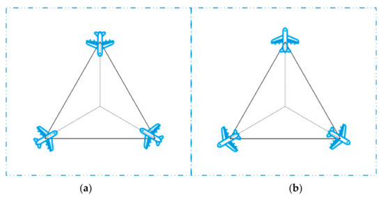
Figure 1.
Different flight trends of aircraft. (a) Convergence trend. (b) Separation trend.
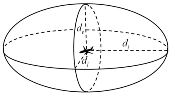
Figure 2.
Ellipsoid flight reserve.
In order to further reflect the conflict relationship between aircraft in the airspace, we derive the three-dimensional speed obstacle method to determine potential flight conflicts. Then, we build a flight conflict network based on the conflict relationship between the aircraft. In the flight conflict network, heading and speed are also important factors for forming the network edge. When a pair of aircraft nodes in the network form a conflict relationship, the two nodes form an edge.
The speed obstacle method essentially divides the speed space between two aircraft into a collision area and a non-collision area. When the relative speed falls into the collision area, it is regarded as a conflict or potential conflict between the two aircraft [36]. This idea is simple and easy to implement. In the following, we introduce the principle of the two-dimensional velocity obstacle model and then build a conflict detection model based on the three-dimensional velocity obstacle method. This method detects the flight conflict between nodes in the flight conflict network and builds the network edge.
Figure 3 shows the principle of the two-dimensional conflict detection model based on the speed obstacle method. Aircrafts and are flying at the same altitude, and the speeds are and , respectively, and the speed of relative to is . Since the two planes are at the same level, the section of the flight protection area of at this level is with point as the center and as the radius.
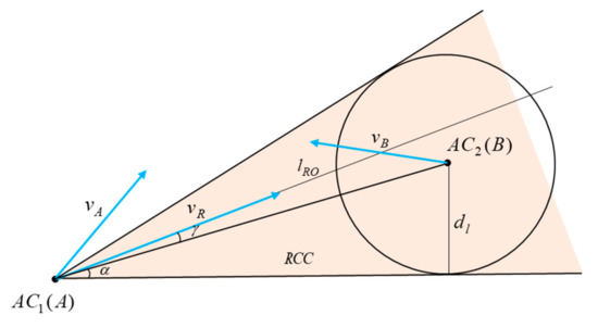
Figure 3.
Two-dimensional collision detection model.
According to the description of the velocity obstacle method above, we can know that there exists a collision cone between two aircraft, and a potential flight conflict occurs when the relative velocity falls in this region. When the initial attitude information of two aircraft is certain, the range of relative velocities that will lead to flight conflict is also determined. In this paper, we define the set of relative velocities that would lead to an aircraft collision as the relative collision cone, and denote it as . The in Figure 3 is the area surrounded by vertex and the tangents between and . When there is an intersection of the extension cord of the relative speed and , it is considered that there is a conflict between two aircraft on the same level.
The above detection method can only detect potential flight conflicts at the same altitude, and it is difficult to judge the conflict relationship between aircraft pairs at different altitudes. Therefore, we combine the ellipsoid flight protection zone and the speed obstacle method to build a three-dimensional conflict detection model. The specific steps are as follows.
The ellipsoid flight protection area around the aircraft is denoted as :
is the coordinates of the target aircraft at the center of the ellipsoid, is the coordinates of the potential conflict aircraft.
As shown in Figure 4, nodes and are flying forward at speeds and , respectively. In the speed obstacle model, the conflict is only related to the aircraft’s relative position and current flight status. Taking as the reference point, makes relative motion, and the relative speed is , and is the extension line of the direction vector . is the set of relative velocities at which collisions occur.
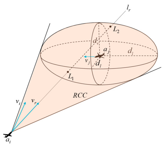
Figure 4.
Three-dimensional collision detection model.
In Figure 4, it is evident that when , and have 2 intersection points. If the extension line of is combined with the ellipsoid surface equation, the intersection point of and the ellipsoid satisfies the following equation system:
The 2 equations in Equation System (3) are in the same coordinate system, which has as the origin point, and is the coordinate of . are the components of the direction vector of on the , , axes.
Let be the number of intersections between and , let be the edge connection discriminant of nodes and .
where, , , are the coefficients of , , and in the polynomial Equation (4), respectively.
Therefore, we can make the following judgments: when , , , the relative speed leaves the relative collision cone; when , , the relative speed does not leave the relative collision cone.
However, there is a problem: when , the relative speed deviating from is also considered to have a conflict risk, and it is necessary to make a supplementary judgment based on Equation (5).
Figure 5 shows the top view of the conflict detection model (in Figure 4). is the projection of the line between nodes and on the horizontal plane . is a circle with as the center and as the radius. and are the included angles between and the tangent and , respectively, then when , the relative speed will not deviate from .
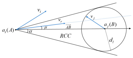
Figure 5.
Top view of the conflict detection model.
Where and are given by:
is the horizontal distance between nodes and .
Through the above analysis, for the flight conflict network, the following judgment can be made: when the two conditions of and are satisfied at the same time, the relative speed will fall within , and there is a risk of conflict between nodes and . At this time, , and nodes and form a connecting edge. Otherwise, , there is no conflict risk between nodes and , and no connecting edge is formed.
2.2. Determine the Edge Weight
The edge weight of network nodes is an indicator used to indicate whether the relationship between nodes at both ends of the edge is vital. In the flight conflict network, the edge weight needs to reflect the urgency of the conflict between the aircraft nodes, and the estimated conflict time can intuitively reflect the intensity of the conflict urgency. When the estimated conflict time is shorter, the conflict urgency is stronger, and this relationship is non-linear. This paper defines the edge weight of a node as:
is the estimated conflict time, which is measured in minutes, and is the edge weight between nodes and .
It can be seen from Equation (8) that the value range of is . has the opposite trend to , when is smaller, is larger; when there is no edge between nodes and , ; when a flight conflict has occurred between nodes and , . This is assuming that the flight protection zone for all aircraft is the ellipsoidal protection zone in Figure 2, and that and . Since the flight conflict network is undirected, it can be obtained that .
Figure 6 shows the positional relationship and conflict relationship of six aircraft in the flight conflict network at the same altitude and within a 30 km × 30 km airspace. In the flight conflict network, the horizontal safety interval is the long radius of the ellipsoidal flight protection zone of 9.26 km. As shown in Figure 6, we can see that the interval between nodes 2 and 6 is less than the horizontal safety interval, and a flight conflict has occurred. There is a potential flight conflict between nodes 1 and 4, 2 and 5, 3 and 5, respectively. As shown in the matrix (9), in the flight conflict network, the edge weight matrix is a symmetric matrix, that is, . The elements not 0 in the matrix represent the flight conflict formed by a pair of aircraft. The larger the element value is, the more urgent the flight conflict is.
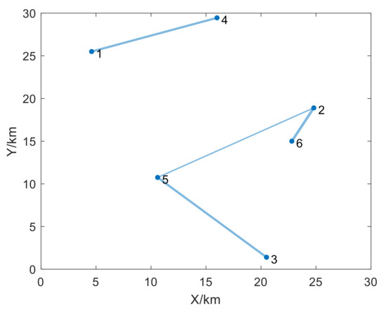
Figure 6.
Flight conflict network (6 nodes).
3. Conflict Resolution Theory Based on “Nucleolar Solution” of Cooperative Game
In the above, we have established a flight conflict network, and the edges and edge weights between nodes in the network can reflect the number and urgency of flight conflicts in the airspace. When the flight status of aircraft nodes in the network changes, the network changes accordingly. Therefore, the change in some indicators in the network before and after conflict resolution can reflect the overall release effect of the resolution strategy. Network efficiency is an indicator to measure the ability of network information communication [37]. When the number of edges in the network is less, and the network efficiency is lower, the strategy has a better resolution effect. In the process of conflict resolution, the entire flight conflict network will pursue the best overall resolution efficiency in order to achieve the purpose of resolving multi-aircraft flight conflicts but ignore the issues of individual fairness and priority. To solve this problem, we introduce the idea of “nucleolar solution” of the cooperative game to realize the benefits balance between the whole network and each aircraft node.
Schmeidler [38] first proposed the concept of nucleolar solution. Its essence is to minimize the degree of dissatisfaction of the alliance while ensuring the optimal welfare of the alliance, so as to achieve a balance between the overall and individual interests [21]. In this paper, all nodes in the entire network are participants in the alliance , and different conflict resolution strategies that satisfy the optimal welfare of the alliance form a strategy set . Let be the alliance cost function, which can reflect the overall satisfaction of the alliance. The smaller is, the higher the overall satisfaction of the alliance. In the process of the game, on the one hand, from the perspective of individuals, they all hope that their avoidance costs are low; on the other hand, from the perspective of the alliance as a whole, it is hoped that the adjusted network conflict will have the best effect. The pursuit of optimal alliance welfare and minimum dissatisfaction among players is consistent with the “nucleolus solution”, taking into account the group’s and individuals’ rationality.
3.1. Network Evaluation Index for Conflict Resolution Performance
In the flight conflict network alliance composed of aircraft nodes, the alliance welfare is related to the overall effect of the conflict resolution strategy. The better the overall conflict resolution effect, the higher the alliance welfare. Therefore, defining an evaluation index that can reflect the overall conflict resolution effect is necessary.
In the study of multi-aircraft conflict resolution, people often take the length of the interval between aircraft pairs as the standard to test the effectiveness of the resolution strategy. They determine that a flight conflict will occur when either the horizontal or vertical interval of the aircraft is less than the safe separation in a future period. However, the network edge can directly reflect the conflict relationship between a pair of aircraft nodes in the flight conflict network. When there is no edge between the two nodes, there is no conflict with the aircraft. Therefore, for the flight conflict network, the following judgment can be made: when the number of edges in the network decreases, the conflict resolution strategy in this scenario is effective. However, there is a problem: although the number of network edges can reflect the number of flight conflicts in the network, it cannot reflect the conflict urgency in the whole network. As shown in Figure 7, both flight conflict networks in Figure 7a,b have 22 edges, but the average edge weight in Figure 7a is 0.3542 and the average edge weight in Figure 7b is 0.3960. In the same flight conflict network, even if the number of edges is the same, the urgency of flight conflicts in the network is different. Taking the number of connected edges of the network as the objective function of conflict resolution lacks gradient.
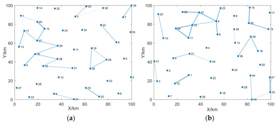
Figure 7.
Flight conflict network with the same number of edges. (a) Flight conflict network A. (b) Flight conflict network B.
In response to the above problems, we extract the comprehensive network index () composed of robustness (), network efficiency (), and clustering coefficient ().
- 1.
- Robustness (R)
In the flight conflict network, the edge weight represents the potential conflict strength of the aircraft nodes at both ends of the edge. The sum of the network’s edge weights can reflect the airspace’s overall flight conflict situation. The definition of robustness is the ability of the system to maintain a normal working state after an error or attack occurs.
is the number of nodes in the network and is the number of nodes that are removed. We did not move nodes out of the network after conflict resolution, and took 0 when performing static analysis on network robustness. The lower the robustness, the less responsive the network is to external disturbances. The node strength is the sum of edge weights of edges connected to a node. In the flight conflict network, the smaller the number of edges and the strength of nodes, the easier it is to resolve them. Therefore, robustness is essential for resolving conflict networks and is the most important relative to the other two indicators.
- 2.
- Network Efficiency (NE)
Network efficiency refers to the structural form of information channels in the communication process and is an indicator to measure the ability of network information communication. The efficiency of information communication between nodes is negatively related to their consumption in the communication channel. In the undirected weighted graph, the closer the relationship between the node pairs is, the greater the edge weight is, so the formula of its network efficiency is:
is the number of connected edges on the shortest path between nodes and , and is the sum of the weights of all edges on the shortest path. In the flight conflict network, the network efficiency reflects the number and intensity of cascading conflicts between aircraft. The higher the , the higher the network complexity, which is the second most important indicator.
- 3.
- Clustering Coefficient (CC)
The agglomeration coefficient is an indicator that reflects the completeness of the connection of small groups of nodes in the network. In an unweighted network, the clustering coefficient can reflect the proportion of node triangles in the network to node triples. For weighted networks with different edge weights, the clustering coefficient of the node can be expressed as:
Equation (12) was proposed by Barthelemy et al. in 2005 [39], where is the clustering coefficient of the node , is the degree of node , and denotes the strength of node . represents the connection between node pairs and . When they form a connected edge, , otherwise . The definition of and is similar to that of .
The agglomeration coefficient of a weighted network is the average value of the agglomeration coefficients of each node in the network, and its formula is:
is the aggregation coefficient value of the i-th node in the network. The agglomeration coefficient in the flight conflict network reflects the proportion of multi-aircraft conflicts in all conflicts. The decrease in its value indicates that the complexity of network conflicts has decreased. Compared with the first two indicators, the importance of the agglomeration coefficient is relatively lower.
In order to determine the weight of each index in , we apply the analytic hierarchy process (AHP) to calculate the weight coefficients of , , and in . The weight vector of robustness, network efficiency, and clustering coefficient is calculated as: [0.5396 0.2970 0.1634], obtaining CI = 0.0046 and simultaneously, and passes the consistency test. Therefore, can be expressed as:
comprehensively considers the number of edges, strength, and node aggregation degree in the flight conflict network. It has both the gradient and the ability to reflect the effect of conflict resolution. It can play an essential role in the process of conflict resolution and help quickly resolve the flight conflict network. When is the smallest, the alliance benefit is the largest.
3.2. Alliance Cost Function
A good conflict resolution strategy should make the resolution cost as small as possible on the premise of ensuring security. In the flight conflict network, the number of participants in the alliance is the number of nodes , nodes in the alliance plays games with each other by adjusting their flight status, and the satisfaction of each aircraft under different escape strategies is different. In this paper, according to the characteristics of the aircraft itself, the cost function is divided into speed cost and heading cost :
is the initial flight speed of node ; and are, respectively, the speed increment and horizontal track inclination of under a certain release strategy; the value ranges of and are both [0, 1].
Then, the alliance cost function can be expressed as:
and are the weight coefficients of the speed term and the angle term in the cost function . The choice of and is a matter of preference selection. For the aircraft itself, compared with increasing or decreasing the speed value, adjusting the heading will make the aircraft deviate from the original trajectory and cause the waste of airspace, and will also involve the problem of trajectory recovery. Therefore, when the conditions are the same, adjusting the heading cost is higher than adjusting the speed. In this paper, we let be 0.7 and let be 0.3.
3.3. Node Priority
In the flight conflict network, some aircraft nodes play a key role in the network, and the priority to release these key nodes will quickly reduce the complexity of the airspace. The edge weight is a network index reflecting the impending effect of node and node , and the node strength is the sum of edge weights of edges connected to a node, which can further reflect the urgency of node conflict. Based on this, we arrange the point strength of each node in descending order. The higher the point strength of the node, the higher its release priority. The point strength of node is:
In the flight conflict network alliance, to make the release strategy fast and reliable, the nodes with high release priority should bear less release cost. That is, the higher the release priority of a node, the higher the cost weight coefficient of the node. We define the cost coefficient of the network node in the alliance as:
According to the definition, the nucleolar solution () of the network alliance after the cooperative game is:
3.4. Consistency of Resolution Strategy Fairness and Optimal Alliance Satisfaction
According to the above description, the basic idea of the “nucleolus solution” is to design a fair solution, which promotes the participants to have higher individual satisfaction without compromising the welfare of the alliance. In Section 3.2, we establish an alliance cost function to reflect the overall satisfaction of the alliance, where the smaller is, the higher the alliance satisfaction. However, there is a problem: if the cost function decreases, the overall satisfaction of the alliance increases, but the individual satisfaction decreases, then the reduction of the alliance cost function will not improve the fairness of the conflict resolution strategy. In order to prove the effectiveness of cost function , we combined the speed obstacle method for mathematical derivation and designed experiments to verify the relationship between cost function and strategy fairness. Specific steps are as follows.
As shown in Figure 8, two aircrafts and at the same altitude fly forward at speeds and , respectively. According to the flight conflict criteria in Section 2, it is obvious that there is a potential flight conflict between the two aircraft in this scenario. According to the definition of the alliance cost function (Equation (17)), the consistency proof of strategy fairness and optimal alliance satisfaction should include: course cost consistency and speed cost consistency.
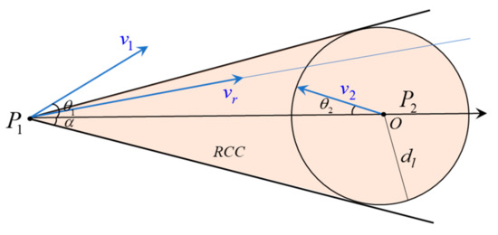
Figure 8.
Flight conflict between two aircraft at the same altitude.
3.4.1. Validation of the Heading Cost Function Consistency
Figure 9a shows the principle of conflict resolution by adjusting the course of . Figure 9b shows the principle of conflict resolution by adjusting the course of . Figure 9c shows the principle of conflict resolution by adjusting the course of and . When the relative speed vectors of the two aircraft coincide with the boundary of after flight state adjustment, the resolution is considered successful.
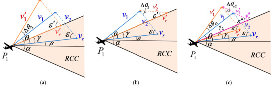
Figure 9.
Principles of course conflict resolution. (a) P1 independently adjusts the heading to resolve the flight conflict. (b) P2 independently adjusts the heading to resolve the flight conflict. (c) P1 and P2 cooperate to resolve the flight conflict by adjusting the course.
The important parameters in the disengagement process are defined as follows: let and be the priority coefficients of and . In the first two resolution modes, let and be their resolution costs, respectively, and let and be the resolution track inclination of and . When and cooperate for course resolution, and are the track inclination of and , respectively, and the cost is .
We first solve for and . As shown in Figure 9a, let and be the initial heading angles of and , respectively, is the angle between and the axis, is the angle between and , is the angle between and , is the angle between and , is the velocity vector of after the course is released, then the heading angle of is after the conflict is resolved.
In the vector triangle , according to the sine theorem, we have:
According to the geometric relationship in Figure 9a, we substitute and into Equation (21). The simplified is:
Next, we substitute Equation (21) into Equation (17) of the cost function. Then, when adjusts the heading independently to resolve the conflict, can be expressed as:
Next, we solve for and . As shown in Figure 9b, the process of independent heading resolution is similar to that of . Let the velocity vector of be and the track inclination of to be after resolution.
According to the geometric relationship in Figure 9a, we have:
By simplifying the above formulas, we can obtain:
In the vector triangle , according to the sine theorem, we have:
Simplified is:
Next, we substitute Equation (27) into Equation (17) of the cost function. When adjusts the heading independently to resolve the conflict, can be expressed as:
Finally, we solve for , , and . As shown in Figure 9c, when and resolve the conflict by cooperatively adjusting their headings, and adjust their respective track inclinations and , so that the relative velocity vector is deflected by angles and ().
According to the geometric relationship in Figure 9c, we have:
In the vector triangle , according to the sine theorem, we have:
We substitute and into Equation (30) and simplify:
Similarly, in the vector triangle , according to the sine theorem, we have:
We substitute Equations (31) and (33) into Equation (17) of the cost function. When and cooperate to adjust the course to resolve the flight conflict, can be expressed as:
In the above, we have derived the alliance cost function of aircraft independent heading conflict resolution and cooperative heading conflict resolution, respectively. In the following, we will design a conflict scenario to verify the consistency of resolution strategy fairness and optimal alliance satisfaction.
As shown in Table 1, we design a conflict scenario. Let us first analyze the relationship between the change in each quantity when the two aircraft cooperate to solve the conflict. is the minimum angle at which the relative speed needs to be deflected when the two aircraft are free from conflict. is the angle at which the relative speed is deflected by adjusting the heading of , and is the angle at which the relative speed is deflected by adjusting the heading of . The units of measurement for , , and are degrees. When two aircraft cooperate to resolve a flight conflict, the total mission can be considered as making the relative velocity deflection of the angle . When is assigned the task of deflecting the relative velocity vector by the angle , then is assigned the task of deflecting the relative velocity vector by the angle . The total task volume is certain, and when the heading deflection angle of gradually increases, increases, and gradually decreases, that is, the task volume undertaken by gradually decreases, and the heading deflection angle of gradually decreases; conversely, when the heading deflection angle of gradually decreases, the task volume undertaken by decreases, and the task volume undertaken by increases, then the heading deflection angle of gradually increases. When , it is considered that the two aircraft have cooperated.

Table 1.
Initial flight status information.
Figure 10 records the change relationship of , , and with on the premise that the aircraft can only adjust the course. The domain of is . It can be seen from Figure 10 that as increases, the two aircraft gradually deepen their cooperation in course release. When they cooperate to resolve the flight conflict, gradually decreases. When is , that is, when aircraft undertakes the task of deflecting the relative velocity vector , the alliance disengagement cost is the smallest, and the is 0.01591; When , , that is, the alliance resolution cost when the two aircraft cooperate to resolve the flight conflict is lower than the alliance release cost when either aircraft or resolves the conflict alone.
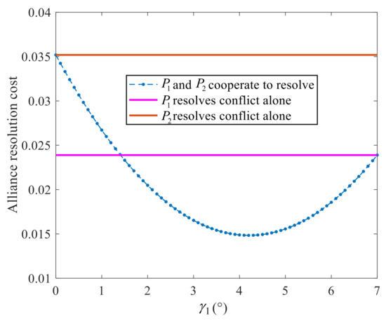
Figure 10.
Heading cost function consistency check.
To sum up, as the degree of cooperation between aircraft pairs in heading and flight conflict resolution gradually deepens, the alliance cost gradually decreases and the alliance satisfaction increases. Therefore, when a pair of aircraft cooperates to adjust the course to resolve the flight conflict, the fairness of the strategy is reflected, the alliance cost is reduced, and the satisfaction is increased. For the heading cost in the alliance cost function , its strategy fairness is consistent with the changing trend of the optimal alliance satisfaction.
3.4.2. Validation of the Speed Cost Function Consistency
Figure 11a shows the principle of conflict resolution by adjusting the speed of . Figure 11b shows the principle of conflict resolution by adjusting the speed of . Figure 11c shows the principle of conflict resolution by adjusting the speed of and . In the process of the first two conditions, let and be the resolution costs of the two scenarios, respectively, and let and be the speed increments of and , respectively. When and cooperate to resolve the flight conflict by adjusting the speed, and are the speed increments of and , respectively, and the cost is .
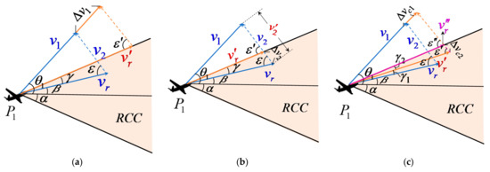
Figure 11.
Principles of speed conflict resolution. (a) P1 independently adjusts the heading to resolve the flight conflict. (b) P2 independently adjusts the heading to resolve the flight conflict. (c) P1 and P2 cooperate to resolve the flight conflict by adjusting the course.
In the vector triangle of Figure 11a, according to the sine theorem, we have:
We substitute into Equation (35) and simplify to obtain:
Next, we substitute the above equation into Equation (17). Then, when adjusts the speed independently to resolve the conflict, can be expressed as:
In the vector triangle of Figure 11b, according to the sine theorem, we have:
We substitute into Equation (38) and simplify to obtain:
can be expressed as:
In the vector triangle of Figure 11c, according to the sine theorem, we have:
We substitute into the above equation and simplify to obtain:
In the vector triangle of Figure 11c, according to the sine theorem, we have:
Next, we simplify the above equation:
We substitute Equations (42) and (44) into Equation (17) of the cost function. When and cooperate to adjust the speed to resolve the flight conflict, can be expressed as:
In the consistency test of speed cost function, we still conduct experiments based on the scenarios in Table 1. Figure 12 records the change relationship of , , and with on the premise that the aircraft can only adjust the speed.
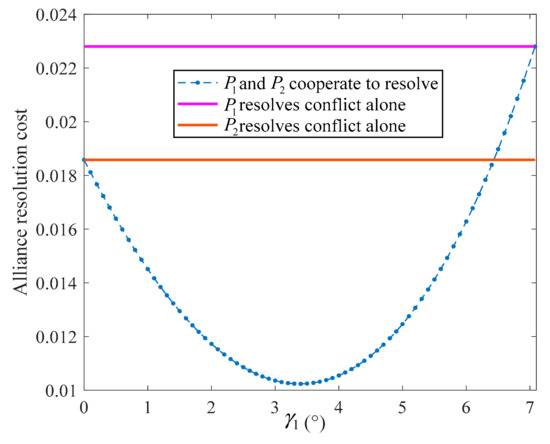
Figure 12.
Speed cost function consistency check.
It can be seen from Figure 12 that as increases, the two aircrafts gradually deepen the cooperation in speed resolution, and the alliance cost under cooperation resolution gradually decreases. When is , reaches the minimum value, and then continues to increase, and the degree of cooperation between the two aircraft gradually decreases. When , , and the speed cost of the two aircrafts cooperating to resolve the conflict is lower than the speed cost of either aircraft or to resolve the conflict alone.
To sum up, with the gradual deepening of the degree of cooperation in speed resolution among the aircraft, the fairness of the resolution strategy is reflected, and the individual satisfaction increases. At the same time, the overall resolution cost of the alliance gradually decreases, and the satisfaction of the alliance increases. Therefore, for speed cost and course cost in alliance cost function , the trend of strategic fairness and alliance satisfaction is consistent. In the process of conflict resolution, if the alliance cost function decreases, the alliance satisfaction increases and the fairness of the resolution strategy improves.
4. Network Conflict Resolution Based on NSGA-II Algorithm
In this paper, we adopt three ways of conflict resolution: course maneuver, speed maneuver, and course–speed compound maneuver. In the process of flight conflict resolution, the smaller the aircraft’s payment cost, the higher the economic benefit and feasibility of the resolution strategy.
In Section 3, we define the alliance cost function and node priority, and the aircraft nodes play games against each other. According to the concept of the nucleolar solution, participants should ensure the maximum overall welfare of the alliance while minimizing the dissatisfaction of the alliance, but the solutions under these two goals are in conflict with each other. In the flight conflict network, adjusting the “key nodes” in the network is the most effective way to resolve the network, but the “key node” has a heavy weight in the alliance cost function, so it is difficult to achieve the optimal value of the two objectives at the same time.
To solve this problem, we introduce the NSGA-II algorithm to solve the solution set of the compromise between two target values, namely the Pareto optimal set. Compared with other multi-objective optimization algorithms, the NSGA-II algorithm not only ensures convergence, but also has potential parallelism. Therefore, its Pareto optimal set can be evenly and widely distributed, ensuring the calculation accuracy and shortening the search time.
4.1. Optimization Objective Function
The optimization objective function is the key to solving the multi-objective optimization problem. In order to make the Pareto optimal set contain the “kernel solution”, the optimization objective function should include and .
Objective function : the comprehensive network index can intuitively reflect the effect of the conflict resolution strategy in the flight conflict network. The smaller the , the better the conflict resolution effect of the resolution strategy. When is equal to 0, there is no flight conflict or potential flight conflict in the network, so taking as one of the objective functions, , can be expressed as:
and are the speed increment and track inclination of the i-th aircraft under the resolution strategy.
Objective function : in the network alliance composed of aircraft nodes, each node needs to pay different costs under different conflict resolution strategies. The lower the resolution cost, the higher the satisfaction of aircraft nodes, and the better the effect of resolution strategies. The alliance cost function can intuitively reflect the total cost of the alliance under a specific disengagement strategy. In Section 3, we proved the consistency between the strategy’s fairness and the alliance’s optimal satisfaction. can give consideration to both group rationality and individual rationality. Therefore, we take as one of the target functions.
is the priority of the i-th aircraft; and are the weight coefficient of the speed item and the angle item in the cost function, respectively.
4.2. Constraints and Coding Methods
4.2.1. Constraints
In reality, the speed variation range of civil aircraft is limited [40]. In order to ensure flight safety and operability in actual work, we make the following assumptions when simulating the flight environment:
- (1)
- We stipulate that the speed variation range of the aircraft during flight is 600–900 km/h.
- (2)
- During the flight conflict resolution process, the flight track inclination angle of a single aircraft should satisfy .
4.2.2. Coding Methods
Combined with the characteristics of genetic algorithms and different conflict resolution methods, we encode the chromosomes of course, speed, and compound maneuver. Figure 13 shows the chromosomes under three conflict resolution methods, and let the number of nodes to be adjusted be q. Figure 13a is the chromosome under course resolution, and the first q bits of the sequence represent the track inclination of each node to be adjusted; Figure 13b is the chromosome under speed resolution, and the first q bits of the sequence represent the speed of q nodes to be adjusted; Figure 13c is the chromosome after compound release, its length is 2q, where the first q bits of the sequence are the heading bit, which records the track inclination angle of the node during the conflict resolution process, the qth bit up to the 2qth bit are the speed bits, which record the resolution speed of each node.
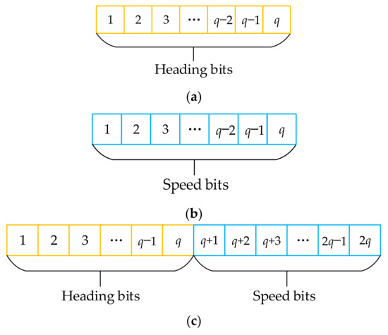
Figure 13.
Chromosomes under three conflict resolution methods. (a) Heading resolution. (b) Speed resolution. (c) Compound resolution.
4.3. Initialize Population
The shorter the calculation time of a resolution strategy, the better the real-time performance of the strategy. In order to shorten the calculation time of the strategy, we derive the initial scheme under different conflict resolution methods, and inject it into the initial population to shorten the distance between the initial solution and the nucleolar solution, so as to improve the real-time performance of the method.
Figure 14 shows the principle of multi-aircraft conflict resolution based on the speed obstacle method. According to the flight conflict judgment criteria in Section 2, when the relative speed vector is within the , the two aircraft form a flight conflict relationship. Therefore, an effective conflict resolution strategy should keep the relative velocity vector out of the . Combining with the definition of the nucleolar solution, we can infer that an effective initial solution strategy should satisfy two conditions: (1) the initial value solution is close to the feasible region of the resolution strategy; (2) the cost of conflict resolution should be as low as possible.
Figure 14.
The principle of multi-aircraft conflict resolution.
In the flight conflict network, let the degree of node be , then the neighbors of are , …, , so that the corresponding weights are , …, . Let , then is the node with the largest edge weight with node . We only change the flight state of node , combined with the speed obstacle method, to relieve the flight conflict between nodes and in three ways.
Next, we define some key variables in the conflict resolution process. When adjusting the heading to resolve the conflict, let the minimum horizontal track inclination of node be (when , adjusts the heading clockwise; when , adjusts the heading counterclockwise). When adjusting the speed of the aircraft to get rid of the flight conflict, let the minimum speed increment of node be (when , accelerates; when , decelerates). When we resolve the flight conflict through the compound release method, the horizontal track inclination of node is and the speed increment is . Then, for any node in the flight conflict network, its initial value of heading resolution is , and its initial value of speed resolution is , and its initial value of compound resolution is and . Then, we derive the initial scheme under the three conflict resolution methods, and the specific steps are as follows.
4.3.1. Initial Value of Course Resolution
As shown in Figure 15, the speeds of the two aircraft nodes and with potential flight conflicts are and , respectively, and the flight conflicts are resolved by adjusting the heading of . In this process, the speed of is not changed, that is, , and only the heading of is adjusted, so that the new relative speed is separated from .
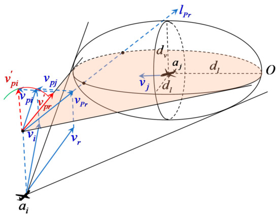
Figure 15.
The principle of course resolution.
Figure 16 shows the principle of resolving the conflict by adjusting the heading on the section plane . Let be the section plane of at the level of , and let and be the projections of and on , respectively. After adjusting the course of , the relative speed disengages from , and the included angle between and is the horizontal track inclination of in the course release strategy. Let be the included angle between and , and let be the included angle between and , and is the included angle between and .
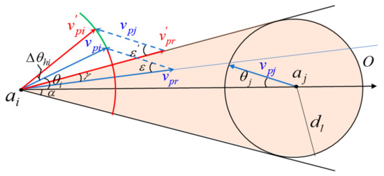
Figure 16.
The principle of course resolution on the section plane.
In the vector triangle , according to the sine theorem and the geometric relationship in Figure 16, we can obtain:
We substitute into Equation (48) and simplify it, then the initial value of the course resolution of node can be expressed as:
4.3.2. Initial Value of Speed Resolution
Similar to the principle of course resolution, in the process of speed resolution, we keep the original course of unchanged, and only adjust the speed of to make the new relative speed detach from .
As shown in Figure 17, there is a flight conflict between and , and is the minimum speed increment of in the speed resolution. Let be the projection of on , and the symbolic definitions of other variables are consistent with those in course resolution.
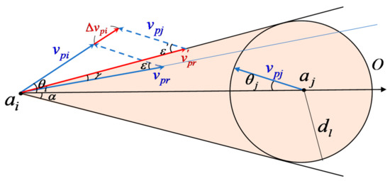
Figure 17.
The principle of speed conflict resolution on the section plane.
In the vector triangle , according to the sine theorem and the geometric relationship in Figure 17, we can obtain:
Then, the initial value in the speed resolution of node can be expressed as:
is the pitch angle of node . When , the node is climbing; when , the node is descending; when , the node is in level flight.
4.3.3. Initial Value of Compound Resolution
In addition to the above two methods, adjusting the aircraft’s heading and speed simultaneously can also avoid flight conflicts. In the process of conflict resolution, the adjustable range of aircraft heading and speed is limited. Compared with heading resolution and speed resolution, the compound resolution method is more applicable and can deal with more flight conflict scenarios.
During the compound disengagement process, the heading and velocity values of are adjusted simultaneously to make the new relative velocity disengage from . In order to facilitate the derivation and analysis, we analyze the adjustment process of the course and speed separately, then the course maneuver and the speed maneuver undertake the task of deflecting the initial relative speed by angles and , respectively ().
As shown in Figure 18, is the node with the largest edge weight with . We analyze the course maneuver and speed maneuver independently, assuming that adjusts the speed first and then adjusts the course. Let be the projection of the relative velocity vector on after adjusts the speed, and let be the projection of the relative velocity vector on after adjusts the course.
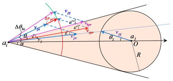
Figure 18.
The principle of compound conflict resolution on the section plane.
In Figure 18, there is the following angular relationship:
In the vector triangle , according to the sine theorem in Figure 18, we can obtain:
We simplify Equation (53) to obtain:
Then, the velocity increment of during compound resolution can be expressed as:
In the vector triangle , according to the sine theorem, we can obtain:
Simplifying Equation (56), then the horizontal track inclination of in the compound solution can be expressed as:
To sum up, we have obtained the initial scheme of node under different resolution methods:
In this section, we derive the initial resolution scheme of any node in the network under three resolution methods. Next, we define the initial population. First, we rank the priority of aircraft nodes in the conflict network from high to low according to Equation (18). Then, we determine the node number to be adjusted according to the priority order. Finally, according to Equation (58), we formulate the corresponding initial resolution scheme and inject it into the initial population. According to the speed range and track inclination range of the nodes in the constraints above, we limit the initial scheme beyond the boundary: when , ; when , ; when , .
4.4. Conflict Resolution Process
As shown in Figure 19, we combine the NSGA-II algorithm to divide the network conflict resolution into the following eight steps.
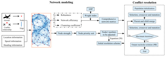
Figure 19.
Algorithm process.
- Step 1: Build the initial network. Based on the flight situation information in the airspace, we construct an initial flight conflict network and calculate the network weight matrix .
- Step 2: Node priority sorting. According to Equation (18), the nodes are sorted from high priority to low priority.
- Step 3: Determine the resolution method and the number of aircraft nodes that need to be adjusted according to the actual control needs.
- Step 4: Initialize the population. The initial resolution scheme is formulated according to Equation (58), and the initial population is generated.
- Step 5: Selection, crossover, and mutation. Calculate the value of the objective function and perform non-dominated sorting, according to the genetic operator operation of crossover and mutation, to generate the offspring population .
- Step 6: Parent and child merge. Merge and to form a new species group with the scale of . Perform the non-dominated relation sorting operation again to screen out the new initial population with the scale of .
- Step 7: Selection, crossover, and variation. The new initial population performs crossover and mutation genetic operators to generate a new offspring population and update the network weight matrix .
- Step 8: Repeat steps 6–7 until the maximum number of iterations of the algorithm is reached. The chromosome with the smallest in the Pareto optimal set is the nucleolar solution (), which is the optimal conflict resolution solution.
5. Simulation and Analysis
In order to verify the effectiveness of the conflict resolution method proposed in this paper, we simulate and analyze the method in the MATLAB environment.
First, we randomly generate 40 aircraft nodes at four altitudes (3900 m, 4200 m, 4500 m, 4800 m) within a 100 km × 100 km airspace, limiting the initial speed of the nodes to a range of 600–900; let be 5 n mile, and let be 2000 ft. Then, according to the rule of establishing the edge of the conflicting network, we establish the edge by determining the conflicting relationship between the aircraft nodes. In the following simulation experiments, we first analyze the difference between the flight conflict network and the aircraft state network. Then, we resolve flight conflict on the basis of this flight conflict network, and compare the resolution effects in different ways.
5.1. Comparison of Two Networks
Figure 20a is the flight conflict network in the initial flight conflict scenario, and Figure 20b is the aircraft state network in this scenario. The aircraft state network takes aircraft as nodes and constructs connected edges when the distance between node pairs is less than 26 km, which is a weightless graph, and the edge weight of this network is the inverse of the horizontal spacing between nodes [23]. Figure 21a,b are the node degree values in the two networks, respectively. Comparing these four graphs, we can see 18 edges in the flight conflict network and 124 in the state network. The degree value of each node is significantly higher than that of each node in the conflict network.
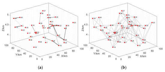
Figure 20.
Two networks for initial flight conflict scenarios. (a) Flight conflict network. (b) Flight state network.
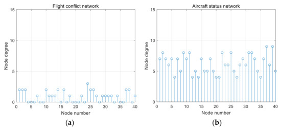
Figure 21.
Node degree of two networks. (a) Flight conflict network. (b) Flight state network.
Compared with the aircraft status network based on aircraft position relationship, the conflict detection method in the flight conflict network can distinguish the aircraft convergence situation and separation situation. The flight conflict network can effectively reduce the number of false alarms in the airspace, especially by avoiding unnecessary energy allocation of controllers in the airspace with high aircraft density.
In Figure 20a, the flight conflict network contains 40 aircraft nodes and 18 edges, of which the numbers of aircraft nodes at the altitude levels of 3900 m, 4200 m, 4500 m, and 4800 m are 8, 9, 13, and 10, respectively. Among these nodes, the pairs of nodes that constitute the edge and are at different altitudes include: , , , , , , , , , , and .
5.2. Conflict Release Effects of Different Resolution Methods
The comprehensive network index () of the initial flight conflict network is 0.1180. Then, we calculate each node’s point strength based on the node priority principle and sort the node priority from high to low. Table 2 shows the priority order of nodes and the weight coefficients of each node in the cost function.
Table 2.
Node priority order.
We use three methods of speed resolution, heading resolution, and compound resolution, respectively, to resolve the flight conflict among 40 aircraft nodes in the flight conflict network. We assume that the controller can deploy up to 10 aircraft under the current air situation and work intensity. In order to improve the timeliness of the resolution strategy, we only adjust the flight status of the first 10 aircraft according to the node priority in Table 2. Then, aircraft nodes that can be adjusted are , , , , , , , , , . This optimization reduces the length of chromosomes and shortens the calculation time.
After determining the adjustable node number, we need to determine the value of and develop the initial resolution scheme. First, we determine the value of . Let , let be the value of for the network after injecting the initial compound resolution scheme into the initial flight conflict network, and let . When is larger, the shorter the distance from the kernel solution for this initial compound resolution scheme, which has the better effect. As shown in Table 3, we recorded the value of when was from 0.1 to 0.9. From Table 3, we can see that the initial compound resolution scheme works best when , so we let .
Table 3.
The value of ΔCNI under different τ.
Then, let us develop the initial resolution scheme. As shown in Table 4, we formulate the initial resolution schemes under different resolution methods according to Equation (58). According to multiple tests, the algorithm converges best when 40% of the initial population contains the initial resolution value. Therefore, we inject a small range of random values around the initial value into 40% of the initial population, and let the population number be 25 and the maximum number of iterations be 300. The following are the optimal schemes under the three resolution methods.
Table 4.
Initial resolution scheme.
5.2.1. Heading Resolution Scheme
Figure 22 records the convergence of objective functions and during the heading resolution process. According to the definition of , the solution with the best conflict resolution effect on the Pareto frontier solution set with level 1 is , that is, is the solution with the smallest in the Pareto frontier solution set. In the solution process, we repeated the algorithm 5 times to obtain the optimal value, and finally obtained the under the heading resolution (in Table 5). Figure 23 shows the flight conflict network after the heading resolution. From Figure 23, we can see that we adjusted 10 aircraft nodes in the process of heading resolution, reduced the number of edges in the network from 18 to 7, and released a total of 7 flight conflicts with nodes at different altitudes: , , , , , , .
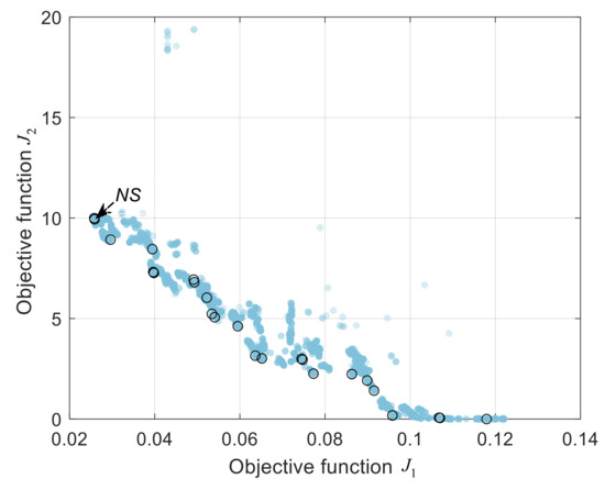
Figure 22.
Convergence of objective function under heading resolution.
Table 5.
Heading conflict resolution scheme.
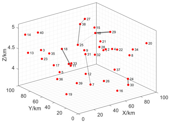
Figure 23.
Flight conflict network after heading resolution.
After the resolution, the comprehensive network index is reduced from 0.1180 to 0.0258, and the alliance release cost was 9.99. In the optimal solution , the horizontal track inclination of node with the highest priority is only adjusted 2.46° Clockwise. Through cooperation with other nodes, the node degree of is reduced from 3 to 1, and its payment cost is small. In the follow-up experiments, we do not repeat the content of the solution many times, and directly use the optimal results in the multiple experiments for verification.
5.2.2. Speed Resolution Scheme
Figure 24 shows the convergence process of the objective functions and during the speed resolution process. The solution with the smallest on the Pareto optimal solution set is . Table 6 records the speed resolution scheme in , and Figure 25 shows the flight conflict network after speed resolution. According to Figure 25 and Table 6, after the speed resolution, is reduced from 0.1180 to 0.1005, only 0.0175 is reduced, and the alliance release cost is far less than the alliance release cost of 9.99 under the heading resolution. Figure 25 shows the flight conflict network after speed resolution. From Figure 25, we can see that the number of edges in the network is reduced from 18 to 14 after the speed resolution, which are all flight conflicts between node pairs at different altitudes. Although the cost of speed resolution is minimal, its release efficiency is much lower than that of heading resolution.
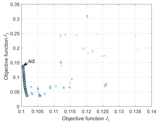
Figure 24.
Convergence of objective function under speed resolution.
Table 6.
Speed conflict resolution scheme.
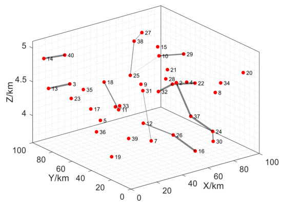
Figure 25.
Flight conflict network after speed resolution.
5.2.3. Compound Resolution Scheme
Figure 26 records the convergence of objective functions and during the compound resolution process, and we mark the position of . Table 7 shows the specific compound resolution scheme, and Figure 27 shows the flight conflict network after compound resolution. Combining Figure 27 and Table 7, we can see that after compound resolution, is reduced from 0.1180 to 0.0210, and the alliance pays the resolution cost during the resolution process. After the conflict is resolved, the number of edges in the conflict network is reduced from 18 to 6, and a total of 12 flight conflicts are resolved, of which 7 flight conflicts are caused by node pairs at different altitudes: , , , , , , . Compared with heading resolution and speed resolution, compound resolution has the better effect, and its optimal solution has a lower resolution cost.
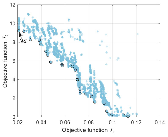
Figure 26.
Convergence of objective function under compound resolution.
Table 7.
Compound conflict resolution scheme.
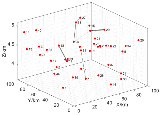
Figure 27.
Flight conflict network after compound resolution.
In order to verify that this multi-aircraft conflict resolution method is also applicable in other scenarios, we record the conflict resolution results of this method in Table 7 for 4 conflict scenarios with different numbers of nodes, assuming that the maximum number of adjustment nodes is half of the total number of nodes. As shown in Table 8, in scenario 1, which contains 20 nodes, the number of connected edges in the flight conflict network is reduced from 10 to 0 after heading and compound resolution, and all 10 flight conflicts are resolved. In scenario 2 containing 40 nodes, when the number of adjustment nodes is 10, the two methods of heading and compound resolution release 12 and 13 flight conflicts, respectively, and the resolution cost in compound resolution is 3.3485 lower than that in heading resolution. When the number of adjustment nodes is 20, both heading resolution and compound resolution can resolve 16 flight conflicts each, and the CNI and resolution cost in compound resolution are lower than in heading resolution. In scenario 3 and scenario 4, both heading resolution and compound resolution show good release effect, which can serve the purpose of reducing airspace complexity and releasing a large number of flight conflicts. With the increase in the number of adjustment nodes, the compound resolution tends to resolve more flight conflicts with a lower resolution cost compared with the heading resolution. In these four scenarios, although speed resolution has a relatively lower resolution cost, its conflict resolution effect is not good.
Table 8.
Results of conflict resolution in different scenarios.
From the above analysis, it can be seen that both heading resolution and compound resolution can find conflict resolution strategies with good release effect and low release cost, but the release effect of speed resolution is not ideal. Therefore, in a complex airspace environment, it is difficult to obtain a good effect of conflict resolution only by adjusting the speed of the aircraft. Compound resolution has the best release effect and can resolve the most flight conflicts. However, due to the longest chromosome length in compound resolution, its algorithm convergence speed decreases.
5.3. The Influence of Alliance Cost Function on Conflict Resolution
In the above experiments, we compared the effects of different resolution methods. The experimental results show that the method has good conflict resolution ability in a complex conflict environment. In order to demonstrate the fairness of the method, we compare the conflict resolution effect and the resolution cost of the method with only conflict resolution as the highest priority goal (GA) and our method in the following experiments.
Figure 28a,b show the changing trends of and with the number of adjusted nodes in the above two methods, respectively. The smaller is, the better the release effect of the release strategy is, and the larger is, the higher the resolution cost of the strategy. From Figure 28a, we can see that as the number of adjustment nodes increases, the of the optimal solution under the two methods are basically the same. However, according to the experimental results in Figure 28b, we can see that the release cost of the nucleolar solution under the proposed method is significantly lower than the release cost of GA. When the number of adjusted nodes is large, the nucleolar solution under the three resolution methods is obviously more fair. When the number of adjustment nodes is greater than 7, compared with GA’s optimal solution, the average release cost of nucleolar solution under heading resolution is reduced by 25.0%, that of speed resolution is reduced by 22.1%, and that of compound resolution is reduced by 30.9%.
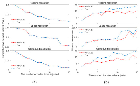
Figure 28.
Comparison of two conflict resolution methods. (a) The variation trend of comprehensive network index with the number of adjusting nodes. (b) The variation trend of alliance release cost with the number of adjusting nodes.
5.4. The Influence of Node Priority and Initial Resolution Scheme on Conflict Resolution
In the above, we prioritized the nodes, shortened the chromosome length by adjusting only 10 key aircraft nodes, and injected initial disentanglement schemes into 40% of the initial population. We obtained effective and low-cost conflict resolution schemes in course resolution and compound resolution. In this section, we will look at the influence of node priority and initial resolution scheme on conflict resolution. As shown in Table 9, we designed four initial population schemes A, B, C, and D to study the impact of adjusting high-priority nodes and injecting initial schemes into the initial population on conflict resolution.
Table 9.
Initial population scheme.
The four initial populations are defined as follows. Scheme A is to randomly select 10 adjusted nodes, and according to different release methods, we randomly generate initial populations within the range of decision variables. Scheme B means that we inject a small range of random values around the initial scheme into 40% of the initial population based on selecting 10 adjusted nodes randomly. Scheme C means that according to the node priority order in Table 2, we select the top 10 nodes with high priority as the deployment nodes, and randomly generate the initial population. Scheme D means that on the basis of selecting the first 10 high-priority nodes, we inject a small range of random values around the initial scheme into 40% of the initial population. Among them, the chromosome length of schemes A and B is 20, and the chromosome length of schemes C and D is 10.
In the process of each iteration of the algorithm, let the position of the minimum value of the objective function be the position of . Figure 29 records the convergence of the under the initial population conditions of A, B, C, and D under the three resolution modes.
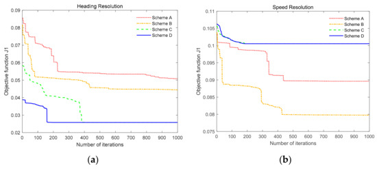
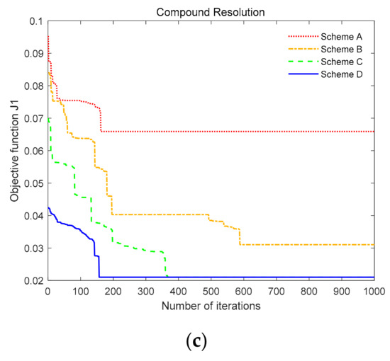
Figure 29.
Convergence of solutions under different initial populations. (a) Heading resolution. (b) Speed resolution. (c) Compound resolution.
As shown in Figure 29a, in the process of heading resolution, compared with scheme A, after injecting 40% of the initial schemes into the population, the convergence speed of the algorithm is slightly improved. After selecting the high-priority nodes, the algorithm convergence speed is greatly accelerated. In scheme D, the algorithm converges rapidly when it iterates to the 159th generation, and when the algorithm iterates to the 164th generation, the heading resolution reaches the optimal solution.
From Figure 29b, we can see that in the process of speed resolution, the algorithms under schemes C and D converge faster, and when it iterates to the 167th generation, the nucleolar solution achieves the optimal release effect. The algorithm has a slower convergence speed under schemes A and B. However, there is the best speed release effect in scheme B. This is mainly because the ability to resolve flight conflicts by adjusting the speed of the aircraft is limited. When the adjusted nodes are limited to a few nodes with high priority, although the convergence speed of the algorithm is improved, the release effect becomes worse.
Figure 29c shows the algorithm convergence of each scheme under the compound solution. We can see that the convergence trend of NS under the compound solution is similar to that of heading resolution, and the order of convergence speed is: D > C > B > A. When the initial population is scheme D, compared with the heading resolution, the compound resolution has a better ability to resolve flight conflicts, but its convergence speed decreases. Through the above analysis, we have made a preliminary judgment on the impact of these two optimization methods on the convergence speed of the algorithm. However, the NSGA-II algorithm is random, and it is difficult to explain the problem clearly in one iteration. In order to reduce the influence of randomness on the overall convergence trend and obtain more accurate conclusions, we conduct the following supplementary experiments. Let us take heading resolution as an example. For every 10 iterations, we will repeat the algorithm 3 times. Figure 30 shows the change in nucleolar solution position in the four groups with the number of iterations under course resolution, which is the result of repeating the algorithm 117 times. Moreover, we take the average of 3 groups of results (in Figure 31a). We repeat the above process for speed and compound resolution and record the average value of the results in Figure 31b,c, respectively.
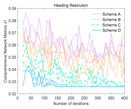
Figure 30.
The example for repeated experimental results.
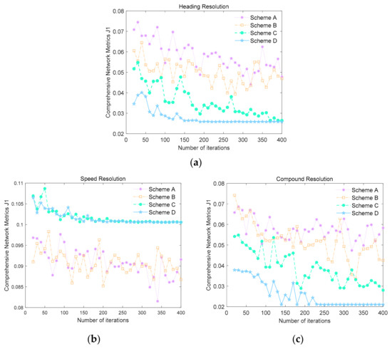
Figure 31.
Comprehensive network index of each initial population under different iteration times. (a) Heading resolution. (b) Speed resolution. (c) Compound resolution.
Combining Figure 29 and Figure 31 for comparative analysis, we can draw the following conclusions: the two optimization methods of only adjusting high-priority aircraft nodes and injecting the initial resolution scheme into the initial population can improve the convergence speed of the algorithm. From Figure 29a,c and Figure 31a,c, we can see that under the heading resolution and compound resolution, adjusting the high-priority nodes can greatly improve the algorithm convergence speed and avoid convergence to the optimal local solution. After injecting the initial scheme, the distance between the initial population and the nucleolar solution is shortened, and the algorithm converges faster. From Figure 29b and Figure 31b, we can see that, under the speed resolution, injecting the initial scheme into the population has little effect on the convergence speed of the algorithm, mainly because the ability to resolve flight conflicts by adjusting the speed is limited. The initial scheme under the speed resolution has difficulty in shortening the distance between the initial population and the nucleolar solution. Furthermore, the average calculation times of course, speed, and compound resolution are 12.04 s, 12.42 s, and 15.17 s, respectively.
To verify that these two optimizations are also applicable to other flight conflict scenarios, we continue our experiments on the basis of the four initial conflict scenarios in Table 8, assuming that the number of adjustment nodes is 10. First, we let be the value of the flight conflict network in the initial scenario, let be the value of in the nucleolar solution with iteration number 1, and let be the time for the algorithm to converge to optimality. The value of can reflect the pros and cons of the initial population to a certain extent. When is relatively small under a certain initial population scheme, it proves that the scheme can shorten the distance between the initial population and the nucleolar solution. The value of can reflect the final convergence of the algorithm under a certain scheme, and the scheme with the smallest has the best effect. The symbol “—” indicates that the solution does not converge to the optimal solution within 2000 iterations.
As shown in Table 10, we record and under different initial populations for the three resolution methods in four conflict scenarios. Scheme D represents the simultaneous use of two optimizations: the selection of high-priority aircraft as deployment nodes and the injection of an initial resolution scheme into the initial population. From Table 10, we can see that is smaller and is lower in scheme D under heading resolution and compound resolution compared to schemes A, B, and C, and the convergence effect of scheme A without any optimization is the worst. This is consistent with the experimental results in Figure 29 and Figure 31. Therefore, we can conclude that both optimizations, adjusting the high-priority nodes and injecting the initial solution into the initial population, can improve the timeliness of the algorithm, and this conclusion holds true in other multi-aircraft conflict scenarios.
Table 10.
Algorithm convergence effect of 4 initial population schemes under different conflict scenarios.
5.5. Comparison of Methods
Table 11 shows the comparison of the multi-aircraft conflict resolution methods proposed in [20,41,42] with this paper, in which [20] combines a cooperative game and particle swarm algorithm to ensure the fairness of the heading resolution strategy, but can only resolve the flight conflicts of fewer than 6 aircraft at the same altitude level and the resolution accuracy is low; [41] improves on the genetic algorithm and can use both heading and speed resolution. The algorithm is improved on the basis of a genetic algorithm, and can use both heading and speed to solve the flight conflict of 6 aircraft. The computation time of this algorithm is 12.35 s for the two-aircraft deconfliction strategy, and the computation time will be significantly increased with the increase in the solution space if the multi-aircraft conflict is to be deconflicted. The method in [42] is able to decouple flight conflicts between 40 UAVs in 3D airspace, but its computation time is 68 s. Compared with the multi-aircraft deconfliction methods in [20,41,42], the method proposed in this paper has a stronger ability to deconflict flights, and when facing a complex conflict scenario with a large number of aircraft and high airspace density, it can complete the adjustment of 10 aircraft and deconflict more than 12 pairs of flight conflicts in 15.17 s, based on high timeliness, strong conflict deconfliction ability, and no secondary flight conflicts. The fairness of the resolution strategy is guaranteed.
Table 11.
Method comparison.
6. Conclusions and Future Prospects
- ConclusionsThis paper establishes a cooperative game conflict resolution model based on the flight conflict network alliance. Combined with the NSGA-II algorithm for iterative optimization, it can quickly resolve flight conflicts between multiple aircraft at different altitudes in the airspace. By analyzing the simulation results, we can draw the following conclusions:
- (1)
- Among the three conflict release methods, the resolution effect of the compound resolution is the best. Moreover, because the aircraft pays less when adjusting the speed, under the premise of the same release effect, the release cost of compound resolution is often lower than that of course resolution. However, the convergence rate of compound resolution decreases due to the longer length of chromosomes. Compared with the compound resolution, the calculation time of heading resolution is shorter, ten aircraft can be adjusted within 12.04 s, and 11 pairs of flight conflicts can be resolved. It has good conflict resolution capability and better timeliness.
- (2)
- When generating the initial population, we only adjust the aircraft nodes with high priority and inject the initial scheme into 40% of the initial population. The experimental results show that the two optimization methods greatly improve the convergence speed of the algorithm, shorten the calculation time, and improve the timeliness of the method.
- (3)
- This paper applies cooperative game theory to flight conflict resolution and demonstrates the feasibility of alliance cost function as a fair solution configuration. The advantage of this fair solution is particularly obvious when the number of adjusted aircraft nodes is large. When faced with a complex conflict scene including 40 aircraft, compared with the release method without considering fairness, the cost of the release strategy under this method is lower under the premise that the effect of conflict resolution is the same. Among them, the alliance resolution costs of heading, speed, and compound maneuvers are reduced by 25.0%, 22.1%, and 30.9%, respectively.
- Future ProspectsIn our future research, we will optimize the following two aspects.On the one hand, we will optimize the computation time of the resolution strategy of each node to improve the real-time performance of the algorithm. For example, we can reduce the size of the solution space by discretizing the decoupling strategy. On the other hand, we will optimize the selection of the adjustment nodes to achieve better conflict resolution. For example, we will determine the adjustment nodes by computing the minimum dominating set of the network.
Author Contributions
Conceptualization, W.Y. and M.W.; methodology, W.Y.; figure, W.Y. and K.B.; data analysis, W.Y. and L.Y.; writing—original draft preparation, W.Y.; writing—review and editing, X.W. and M.W.; supervision, X.W. and M.W.; project administration, M.W. and X.W.; funding acquisition, X.W. All authors have read and agreed to the published version of the manuscript.
Funding
This work was funded by the National Science Foundation of China grant number 71801221.
Data Availability Statement
The data that support the findings of this study are available from the corresponding author, X.W., upon reasonable request.
Conflicts of Interest
The authors declare no conflict of interest.
References
- Durand, N.; Barnier, N. Does ATM need centralized coordination? Autonomous conflict resolution analysis in a constrained speed environment. Air Traffic Control Q. 2015, 23, 325–346. [Google Scholar] [CrossRef][Green Version]
- Zhang, M.; Yu, J.; Zhang, Y.F. Flight conflict resolution during low-altitude rescue operation based on ensemble conflict models. Adv. Mech. Eng. 2017, 94, 168781401769665. [Google Scholar] [CrossRef]
- Wu, M.G.; Wang, Z.K.; Wen, X.X. Aircraft conflict resolution model based on geometric optimization. J. Phys. Conf. Ser. Eng. 2019, 1168, 022034. [Google Scholar] [CrossRef]
- Fan, X.J.; Guo, Y.J.; Liu, H. Improved Artificial Potential Field Method Applied for AUV Path Planning. Math. Probl. Eng. 2020, 2020, 6523158. [Google Scholar] [CrossRef]
- Tomlin, C.; Pappas, G.J.; Sastry, S. Conflict resolution for air traffic management: A study in multiagent hybrid systems. IEEE Trans. Autom. Control 1998, 43, 509–521. [Google Scholar] [CrossRef]
- Tang, X.M.; Ji, X.Q.; Li, T. Key Technology in Multi-UAV Conflict Detection and Resolution Strategy. Trans. Nanjing Univ. Aeronaut. Astronaut. 2020, 37, 175–186. [Google Scholar]
- Cai, J.L.; Zhang, N. Mixed Integer Nonlinear Programming for Aircraft Conflict Avoidance by Applying Velocity and Altitude Changes. Arab. J. Sci. Eng. 2019, 40, 8893–8903. [Google Scholar] [CrossRef]
- Hong, Y.; Choi, B.; Oh, G. Nonlinear conflict resolution and flow management using particle swarm optimization. IEEE Trans. Intell. Transp. Syst. 2017, 18, 3378–3387. [Google Scholar] [CrossRef]
- Han, Y.X.; Tang, X.M.; Han, S.C. Conflict resolution model of optimal flight for fixation airway. J. Traffic Transp. Eng. 2012, 12, 115–120. [Google Scholar]
- Tang, X.M.; Chen, P.; Li, B. Optimal air route flight conflict resolution based on receding horizon control. Aerosp. Sci. Technol. 2016, 50, 77–87. [Google Scholar] [CrossRef]
- Xiang, Z.; Zhang, W.Q.; He, D.Y. A Centralized Algorithm with Collision Avoidance for Trajectory Planning in Preflight Stage. Int. J. Aerosp. Eng. 2021, 50, 6657464. [Google Scholar] [CrossRef]
- Pietrabissa, A.; Ricciardi Celsi, L.; Cimorelli, F. Lyapunov-Based Design of a Distributed Wardrop Load-Balancing Algorithm with Application to Software-Defined Networking. IEEE Trans. Control Syst. Technol. 2019, 27, 1924–1936. [Google Scholar] [CrossRef]
- Tomlin, C.; Ma, Y.; Sastry, S. Free flight in 2000: Games on Lie groups. In Proceedings of the IEEE Conference on Decision & Control, Tampa, FL, USA, 18 December 1998. [Google Scholar]
- Teo, R.; Tomlin, C. Computing provably safe aircraft to aircraft spacing for closely spaced parallel approaches. In Proceedings of the Digital Avionics Systems Conference, Philadelphia, PA, USA, 7–13 October 2000. [Google Scholar]
- Archibald, J.K.; Hill, C.; Jepsen, N.A. A satisficing approach to aircraft conflict resolution. IEEE Trans. Syst. Man Cybern. Part C 2008, 38, 510–521. [Google Scholar] [CrossRef]
- Guan, X.M.; Lv, R.L. Aircraft conflict resolution method based on satisfying game theory. Acta Aeronaut. Astronaut. Sin. 2017, 38, 721475. [Google Scholar]
- Kim, N.; Yoon, Y. Cooperative UAVs Collision Avoidance Based on Satisficing Theory. Int. J. Aeronaut. Space Sci. 2019, 20, 978–986. [Google Scholar] [CrossRef]
- Chen, X.; Wan, Y.; Lao, S.Y. Graphical Modeling and Simulation for a Multi-Aircraft Collision Avoidance Algorithm based on Collaborative Decisions. Symmetry 2020, 12, 985. [Google Scholar] [CrossRef]
- Sislak, D.; Volf, P.; Pechoucek, M. Agent-Based Cooperative Decentralized Airplane-Collision Avoidance. IEEE Trans. Intell. Transp. Syst. 2011, 12, 36–46. [Google Scholar] [CrossRef]
- Jiang, X.R.; Wu, M.G.; Wen, X.X. Conflict resolution of multi-aircraft based on the cooperative game. Syst. Eng. Electron. 2018, 40, 2482–2489. [Google Scholar]
- Zhang, X.; Sun, H.; Xu, G.J. On the core, nucleolus and bargaining sets of cooperative games with fuzzy payoffs. J. Intell. Fuzzy Syst. 2019, 36, 6129–6142. [Google Scholar] [CrossRef]
- Cacace, F.; Mattioni, M.; Monaco, S.; Ricciardi Celsi, L. Topology-induced containment for general linear systems on weakly connected digraphs. Automatica 2021, 131, 109734. [Google Scholar] [CrossRef]
- Jiang, X.R.; Wen, X.X.; Wu, M.G. A complex network analysis approach for identifying air traffic congestion based on independent component analysis. Phys. A Stat. Mech. Its Appl. 2019, 523, 364–381. [Google Scholar] [CrossRef]
- Wang, H.Y.; Xu, X.H.; Zhao, Y.F. Empirical Analysis of Aircraft Clusters in Air Traffic Situation Networks. Proc. Inst. Mech. Eng. Part G J. Aerosp. 2017, 231, 1718–1731. [Google Scholar] [CrossRef]
- Liu, S.Y.; Li, Z.F.; Zhong, J.L. Percolation transition in temporal airport network. Chin. J. Aeronaut. 2020, 33, 219–226. [Google Scholar] [CrossRef]
- Wang, Z.K.; Wen, X.X.; Wu, M.G. Identification of Key Nodes in Aircraft State Network Based on Complex Network Theory. IEEE Access 2019, 7, 60957–60967. [Google Scholar]
- Yang, Y.Z.; Wang, X.; Chen, Y. Identifying Key Nodes in Complex Networks Based on Global Structure. IEEE Access 2020, 8, 32904–32913. [Google Scholar] [CrossRef]
- Wu, M.G.; Li, J.W.; Wen, X.X. Minimum connected dominating set solving algorithm based on immune particle swarm. J. Huazhong Univ. Sci. Technol. (Nat. Sci. Ed.) 2019, 47, 90–95. [Google Scholar]
- Yang, L.S.; Yin, W.; Hu, M.H. Empirical exploration of air traffic and human dynamics in terminal airspaces. Transp. Res. Part. C Emerg. Technol. 2017, 84, 219–244. [Google Scholar] [CrossRef]
- Miao, S.X.; Cheng, C.Q.; Zhai, W.X. A Low-Altitude Flight Conflict Detection Algorithm Based on a Multilevel Grid Spatiotemporal Index. ISPRS Int. J. Geo-Inf. 2019, 8, 289. [Google Scholar] [CrossRef]
- Zhang, M.Y.; Liang, B.Y.; Wang, S. Analysis of flight conflicts in the Chinese air route network. Chaos Solitons Fractals 2018, 122, 97–102. [Google Scholar] [CrossRef]
- Chen, X.W.; Steven, J.L.; Shimon, Y.N. A framework of enroute air traffic conflict detection and resolution through complex network analysis. Comput. Ind. 2011, 62, 787–794. [Google Scholar] [CrossRef]
- Huang, Y.; Tang, J.; Lao, S.Y. Cooperative Multi-UAV Collision Avoidance Based on a Complex Network. Appl. Sci. 2019, 9, 3943. [Google Scholar] [CrossRef]
- Wan, Y.J.; Tang, J.; Lao, S.Y. Distributed Conflict Detection and Resolution Algorithms for Multiple UAVs Based on Key-Node Selection and Strategy Coordination. IEEE Access 2019, 7, 42846–42858. [Google Scholar] [CrossRef]
- Menon, P.K.; Sweriduk, G.D.; Sridhar, B. Optimal strategies for free-flight air traffic conflict resolution. J. Guid. Control Dyn. 1999, 2, 202–211. [Google Scholar] [CrossRef]
- Sun, F.; Chen, Y.; Xu, X. Velocity obstacle–based conflict resolution and recovery method. Aeronaut. J. 2021, 126, 345–364. [Google Scholar] [CrossRef]
- Liu, A.F.; Nie, H.W.; Wu, X.Y. Optimization Deployment Algorithm for Network Efficiency of Linear Wireless Sensor Networks. Comput. Sci. 2009, 36, 83–87. [Google Scholar]
- Schmeidler, D. The nucleolar of a characteristic function game. SIAM J. Appl. Math. 1968, 17, 1163–1170. [Google Scholar] [CrossRef]
- Barthelemy, M.; Barrat, A.; Pastor-Satorras, R. Dynamical patterns of epidemic outbreaks in complex heterogeneous networks. J. Theor. Biol. 2005, 235, 275–288. [Google Scholar] [CrossRef] [PubMed]
- Durand, N. Constant speed optimal reciprocal collision avoidance. Transp. Res. Part. C Emerg. Technol. 2018, 36, 366–379. [Google Scholar] [CrossRef]
- Wu, J.; Zhang, J.J. Conflict resolution of multiple airplanes in free flight based on the genetic algorithm. CAAI Trans. Intell. Syst. 2013, 8, 16–20. [Google Scholar]
- Tang, J.; Fan, L.J.; Lao, S.Y. Collision Avoidance for Multi-UAV Based on Geometric Optimization Model in 3D Airspace. Arab. J. Sci. Eng. 2014, 39, 8409–8416. [Google Scholar] [CrossRef]


Publisher’s Note: MDPI stays neutral with regard to jurisdictional claims in published maps and institutional affiliations. |
© 2022 by the authors. Licensee MDPI, Basel, Switzerland. This article is an open access article distributed under the terms and conditions of the Creative Commons Attribution (CC BY) license (https://creativecommons.org/licenses/by/4.0/).