
2D Discrete Hodge–Dirac Operator on the Torus


Department of Mathematics, Faculty of Civil Engineering, Environmental and Geodetic Sciences, Koszalin University of Technology, Sniadeckich 2, 75-453 Koszalin, Poland
Symmetry 2022, 14(8), 1556; https://doi.org/10.3390/sym14081556
Submission received: 28 June 2022
/
Revised: 25 July 2022
/
Accepted: 26 July 2022
/
Published: 28 July 2022
(This article belongs to the Special Issue Functional Analysis, Fractional Operators and Symmetry/Asymmetry)
Abstract
:We discuss a discretization of the de Rham–Hodge theory in the two-dimensional case based on a discrete exterior calculus framework. We present discrete analogues of the Hodge–Dirac and Laplace operators in which key geometric aspects of the continuum counterpart are captured. We provide and prove a discrete version of the Hodge decomposition theorem. The goal of this work is to develop a satisfactory discrete model of the de Rham–Hodge theory on manifolds that are homeomorphic to the torus. Special attention has been paid to discrete models on a combinatorial torus. In this particular case, we also define and calculate the cohomology groups.
1. Introduction
The choice of technique to approximate the solution of partial differential equations depends on the discretization scheme. In recent years, there has been a growing interest within the computing community in discrete models that preserve the geometric structure of their continuum counterparts [1,2,3,4,5]. Ideally, a geometric discretization scheme should share the same properties with the continuum, but practically it is difficult to achieve. Computational methods often fail to preserve some fundamental geometric structures of underlying continuum models. Usually, there are difficulties with definitions of discrete counterparts of the Hodge star and of the exterior product of differential forms. Various approaches to discretizing exterior calculus have been proposed in the literature (see, e.g., [6,7,8,9,10,11]). Most of them use simplicial chains and cochains as basic constructs for the discrete exterior calculus. An approach based on the use of the Whitney map, which maps chains to differential forms, was developed in [6,7,8,11]. Another approach to discrete exterior calculus was presented in [5,9,10]. These authors consider discrete forms as real-valued functions on the space of simplicial chains. Recently, also, a quite general framework of discrete calculus based on a new type of discrete geometry (script geometry) was proposed in [12].
In this article, we follow the approach that was initially introduced by Dezin [13] and later further developed in the author’s previous papers [14,15,16,17]. We present a discretization scheme using cochains over rectangular meshes as the discrete representation of differential forms. Our approach is also different from those available in the literature in terms of definitions of the Hodge star and a discrete analogue of the exterior product. The discrete analogue of the exterior product is defined in a way that allows the Leibniz-type rule to be valid for a discrete analogue of the differential when it acts on this product of discrete forms.
Let denote the graded vector space of smooth differential forms on , where denotes the subspace of r-forms, . Let be the exterior derivative. The codifferential is defined by , where ∗ is the Hodge star operator such that and . The operator
is called the Hodge–Dirac operator on . The Laplacian is defined by
Our goal is to develop a satisfactory discrete model of the de Rham–Hodge theory on manifolds which are homeomorphic to the torus. We consider a chain complex as a combinatorial model of . Supplemented by discrete analogues of the exterior derivative, the Hodge star operator, and the exterior product acting on cochains, it provides all the basic ingredients for the calculus of discrete counterparts of differential forms. We show that discrete analogues of the operators (1) and (2) have the same properties as those in the continual case. We formulate and prove a discrete version of the Hodge decomposition theorem and provide an example which illustrates how cohomology groups are calculated for our discrete model. Note that our construction of discrete versions of the Hodge–Dirac and Laplace operators is very similar to one proposed in Section 5 of [12]. Matrix forms of these discrete operators on the torus are the same in both cases. The difference between the two approaches is in the definitions of discrete Hodge–Dirac and Laplace operators. In [12], the definitions are given in terms of the exterior derivative and boundary operators, while we define these operators in terms of the exterior derivative and its adjoint, as in the continual theory. We believe our approach is also simpler than previous ones.
2. Discrete Model
In this section, we briefly review the construction of a discrete exterior calculus framework, which was initiated in [13] and developed in, e.g., [14,15].
The starting point of consideration is a two-dimensional chain complex (a combinatorial model of ). Let the sets and , , be the generators of free abelian groups of zero-dimensional and one-dimensional chains of the one-dimensional complex . The free abelian group is understood as the direct sum of infinity cyclic groups generated by , . The boundary operator is the homomorphism defined by and the boundary of every zero chain is defined to be zero. Geometrically, we can interpret the zero-dimensional basis elements as points of the real line and the one-dimensional basis elements as open intervals between points. We call the complex C a combinatorial real line. Let the tensor product
be a combinatorial model of the two-dimensional Euclidean space . The two-dimensional complex contains the free abelian groups of r-chains, , generated by the basic elements
where . It is convenient to introduce the shift operators in the set of indices by
The boundary operator is given by
The definition (4) is extended to arbitrary chains by linearity.
Let be a complex of cochains with real coefficients. The cochain complex is the dual object to the chain complex . It has a similar structure to and consists of cochains of dimension 0, 1 and 2. Then, can be expressed by
where is the set of all r-cochains. We will call cochains forms (or discrete forms), emphasizing their relationship with differential forms. Then, the complex is a discrete analogue of the grade algebra of differential forms . Denote by , and are the basis elements of , and , respectively. The pairing is defined with the basis elements of by the rule
where is the Kronecker delta. The operation (5) is linearly extended to arbitrary chains and cochains. Let , then we have
where , , and are real numbers for any .
The coboundary operator is defined by
where . The operator is an analog of the exterior differential. From the above it follows that
By (4) and (5) we can calculate
where and are the difference operators defined by
Here, is a component of and is given by (3). Note that .
We now consider a multiplication of discrete forms, which is an analogue of the exterior multiplication for differential forms. Denote this multiplication by ∪. For the basis elements of , the ∪-multiplication is defined as follows
supposing the product to be zero in all other cases. The operation is extended to arbitrary forms by linearity. It is important to note that this definition leads to the following discrete counterpart of the Leibniz rule for differential forms.
Proposition 1.
Let and . Then
This was proved by Dezin [13].
Define the operation by the rule
Again, the operation is extended to arbitrary forms by linearity. This operation is a discrete analogue of the Hodge star operator. It is true that for any , we have
Consider the two-dimensional finite chain with unit coefficients of the form
This chain imitates a rectangle. Using (4), we have
Then, for forms of the same degree r, the inner product over the set V is defined by the rule
For forms of different degrees, the product (16) is set equal to zero. From (13) and (5), we have
Proposition 2.
Let and , . Then, we have
where
is the operator formally adjoint of .
The operator given by (18) is a discrete analogue of the codifferential . For the 0-form , we have . It is obvious from (18) that for any Using (8)–(10), (12) and (18), we can calculate
In the particular case , the Equality (17) can be expressed as
where . The similar equality holds in the case .
It should be noted that the relation (17) includes not only the forms with the components and , where the subscripts would run only over the values from (14), but also the components , , , , , , and .
Let us set
For r-forms satisfying conditions (21), the inner product (16) generates the finite-dimensional Hilbert spaces . Now, we consider the operators
Proposition 3.
Let and , . Then, we have
3. Discrete Hodge Decomposition
In this section, we discuss properties of discrete analogues of the Laplacian and Hodge–Dirac operators using concepts introduced in the previous section. We also present a discrete version of the Hodge decomposition theorem, emphasizing that it provides an exact counterpart to the continuum theory.
Let us consider the operator
This is a discrete analogue of the Laplacian (2).
Proposition 4.
For any r-form , we have
and if and only if .
Proof.
By Proposition 3, one has
where denotes the norm and
From this, if then and . It gives and . Hence,
□
Corollary 1.
if and only if and .
Proposition 5.
The operator is self-adjoint, i.e.,
Proof.
By (22), it is obvious. □
Consider the spaces
and
By analogy with the continuum case, the discrete r-form is called closed if and exact if .
Proposition 6.
For each , we have the direct sum decomposition
Proof.
The space decomposes into
where and are the orthogonal complements of the corresponding spaces. For any , we have and
for any . Therefore, is orthogonal to . It follows that
Similarly, we find . Hence, (23) becomes
where
By Corollary 1, we have .
Similar reasonings apply to the spaces and . Thus, we have
since and . □
The Proposition 6 is a discrete version of the well-known Hodge decomposition theorem (see, e.g., [18]).
Let be an inhomogeneous discrete form, i.e., , where . The inner product (16) can be extended to an inner product of inhomogeneous discrete forms by the rule
where . The inner product (24) generates the finite-dimensional Hilbert space . It is true that
By Proposition 6, the following holds
where
and
The discrete Hodge–Dirac operator is defined as
Proof.
By (22), it is obvious. □
Proposition 8.
Proof.
Proposition 9.
For any inhomogeneous form , there exists a unique form which is a solution to the equation
Proof.
Since the operator (26) is self-adjoint and is a finite-dimensional Hilbert space, the existence of the solution is a consequence of the uniqueness of the solution and vice versa. By Proposition 8, implies . From this and by (25), the uniqueness of the solution of Equation (28) follows immediately. □
Corollary 2.
If is a solution of Equation (28), then the following holds
where c is a constant, , and is the projection of Ω onto .
4. Combinatorial Torus
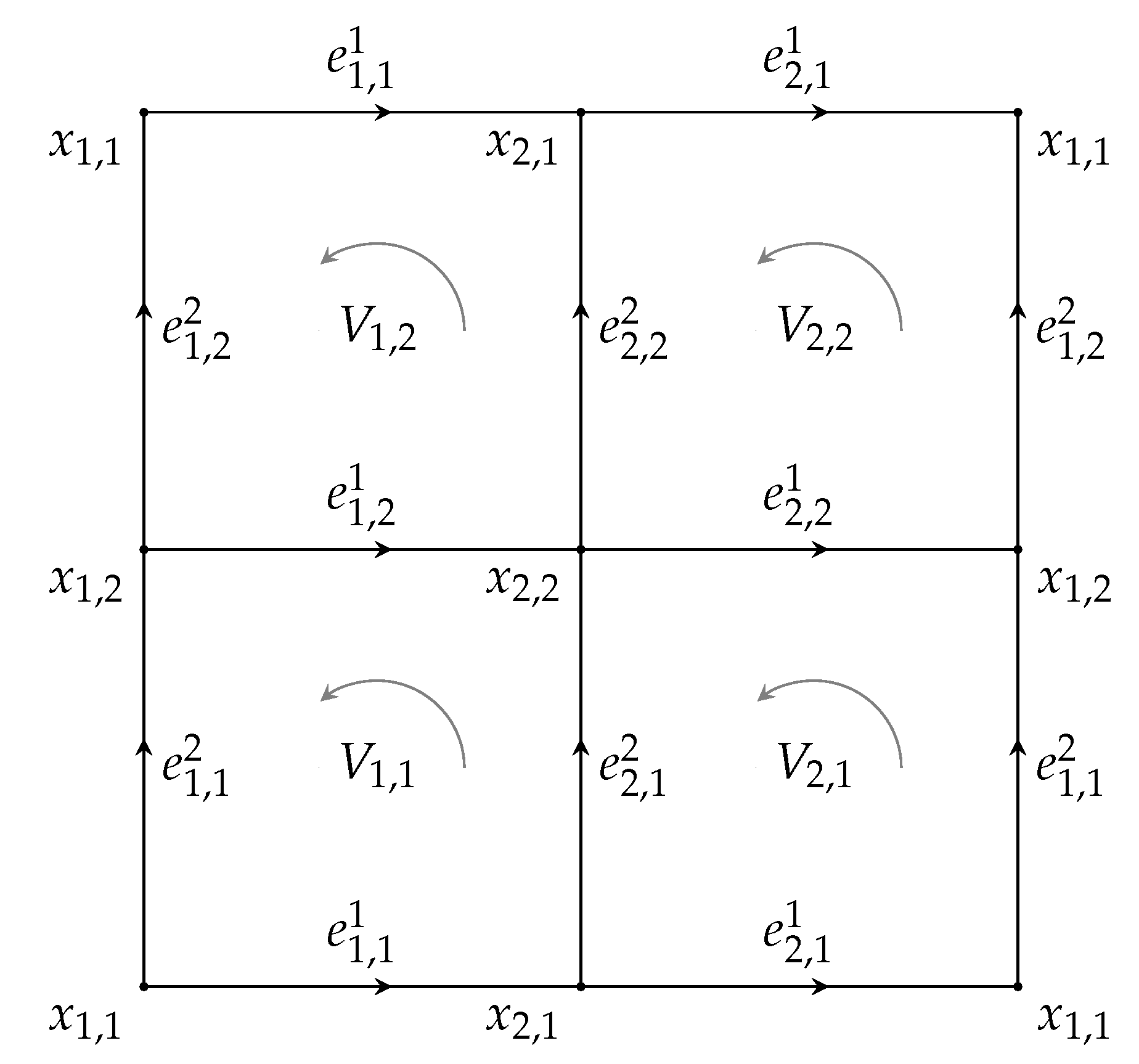
In this section, we consider an example of the discrete model of the torus in detail. We recall that the torus can be regarded as the topological space obtained by taking a rectangle and identifying each pair of opposite sides with the same orientation. Let us consider the partitioning of the plane by the straight lines and , where . Denote by , an open square bounded by the lines and , where is given by (3). Denote the vertices of by , . Let and be the open intervals and , respectively. These geometric objects can be identified with the combinatorial objects considered in previous sections. We identify the collection with V given by (14) and let . In this case, the conditions (21) take the form
where and . If we identify the points and the intervals on the boundary of V in the following way
we obtain the geometric object which is homomorphic to the torus (see Figure 1). Denote by the complex , which corresponds to the introduced geometric object. We call a combinatorial torus.
It is clear that by (30), the conditions (29) hold for any r-form on the combinatorial torus. The Hilbert space considered in previous sections can be regarded as the space of cochains of the complex dual to .
Let us now consider the forms , and , that is
By (30), for these forms, the formulas (8), (9), (19) and (20) become
It should be noted that the formulas above can be expressed in the matrix form. Let us introduce the following row vectors
Denote by , a corresponding column vector. Then, we have
where
and , are the transpose of A, B.
The discrete Hodge–Dirac operator (26) on the combinatorial torus can be represented by the following block matrix
where 0 is a zero square matrix of the corresponding size.
In the same way, the discrete Laplacian on the combinatorial torus can be written as
where
Let us define analogues of the cohomology groups of the combinatorial torus . The quotient space of the linear space of closed r-forms
modulo the subspace of exact r-forms
is called the r-th cohomology group of , that is,
Two closed r-forms and are cohomologous, , if, and only if, they differ by an exact form, i.e.,
An element of is, thus, an equivalence class of closed r-forms , defined by the equivalence relation ∼. These equivalence classes endow with a group structure.
Calculation of . Since there are no -forms, a 0-form can never be exact, i.e., . If , then . By (31), it follows immediately that . Hence,
where is a constant. Thus, is isomorphic to the group generated by one independent generator which is isomorphic to , and we write .
Calculation of . Let . Then, for some . From (31), we have
It follows that
Hence, any form can be written as
Let now be a closed 1-form, i.e., and . By (32), the requirement means that
From this, we obtain
Hence, any form can be written as
This yields
where
and note that . Hence,
This means that has two independent generators. Thus, .
Calculation of . A 2-form
is an element of if for some 1-form . Using (32), gives rise to
Adding these equations, we obtain
Hence, any element can be written as
Since for any 2-form , . Any element of can be expressed as
where
Thus,
since . This means that has only one independent generator; so .
5. Conclusions
We proposed a discretization scheme based on the use of the differential forms calculus.
This scheme was applied to the Hodge–Dirac operator in the two-dimensional case and the
properties of the discrete Hodge–Dirac operator were discussed. A discrete version of the
Hodge decomposition theorem was proved. The proposed discrete model was applied to
the combinatorial torus and the cohomology groups were calculated. Moreover, it was also
shown that the cohomology groups in the discrete case are exactly the same as those in the
continuum one. Issues of convergence and numerical implementation remain to be studied
in detail. We finish by remarking that the content of this work can be developed for the
n-dimensional torus. These problems are the subject of current work in progress.
Funding
This research received no external funding.
Data Availability Statement
Not applicable.
Conflicts of Interest
The author declares no conflict of interest.
References
- Arnold, D.N.; Falk, R.S.; Winther, R. Finite element exterior calculus, homological techniques, and applications. Acta Numer. 2006, 15, 1–155. [Google Scholar] [CrossRef] [Green Version]
- Arnold, D.N.; Falk, R.S.; Winther, R. Finite element exterior calculus: From Hodge theory to numerical stability. Bull. Amer. Math. Soc. 2010, 47, 281–354. [Google Scholar] [CrossRef] [Green Version]
- Ayoub, R.; Hamdouni, A.; Razafindralandy, D. A new Hodge operator in discrete exterior calculus. Application to fluid mechanics. Commun. Pure Appl. Anal. 2021, 20, 2155–2185. [Google Scholar] [CrossRef]
- Stern, A.; Leopardi, P. The abstract Hodge-Dirac operator and its stable discretization. SIAM J. Numer. Anal. 2016, 54, 3258–3279. [Google Scholar]
- Mohamed, M.S.; Hirani, A.N.; Samtaney, R. Discrete exterior calculus discretization of incompressible Navier–Stokes equations over surface simplicial meshes. J. Comput. Phys. 2016, 312, 175–191. [Google Scholar] [CrossRef] [Green Version]
- Dodziuk, J. Finite-difference approach to Hodge theory of harmonic forms. Am. J. Math. 1976, 98, 79–104. [Google Scholar] [CrossRef] [Green Version]
- Sen, S.; Sen, S.; Sexton, J.C.; Adams, D. A geometric discretisation scheme applied to the Abelian Chern-Simons theory. Phys. Rev. E 2000, 61, 3174–3185. [Google Scholar] [CrossRef] [Green Version]
- Wilson, S.O. Differential forms, fluids, and finite models. Proc. Am. Math. Soc. 2011, 139, 2597–2604. [Google Scholar] [CrossRef] [Green Version]
- Desbrun, M.; Hirani, A.N.; Leok, M.; Marsden, J.E. Discrete exterior calculus. arXiv 2005, arXiv:math/0508341v2. [Google Scholar]
- Desbrun, M.; Kanzo, E.; Tong, Y. Discrete differential forms for computational modeling. In Discrete Differential Geometry. Oberwolfach Seminars; Bobenko, A.I., Schroder, P., Sullivan, J.M., Ziegler, G.M., Eds.; Birkhäuser Verlag: Basel, Switzerland, 2008; Volume 38, pp. 287–323. [Google Scholar]
- Teixeira, F.L. Differential forms in lattice field theories: An overview. ISRN Math. Phys. 2013, 2013, 487270. [Google Scholar] [CrossRef] [Green Version]
- Cerejeiras, P.; Kähler, U.; Sommen, F.; Vajiac, A. Script Geometry. In Modern Trends in Hypercomplex Analysis. Trends in Mathematics; Bernstein, S., Kähler, U., Sabadini, I., Sommen, F., Eds.; Birkhäuser: Cham, Switzerland, 2016; pp. 79–110. [Google Scholar]
- Dezin, A.A. Multidimensional Analysis and Discrete Models; CRC Press: Boca Raton, FL, USA, 1995. [Google Scholar]
- Sushch, V. Green function for a two-dimensional discrete Laplace-Beltrami operator. Cubo 2008, 10, 47–59. [Google Scholar]
- Sushch, V. A discrete model of the Dirac-Kähler equation. Rep. Math. Phys. 2014, 73, 109–125. [Google Scholar] [CrossRef] [Green Version]
- Sushch, V. A discrete Dirac-Kähler equation using a geometric discretisation scheme. Adv. Appl. Clifford Algebr. 2018, 28, 72. [Google Scholar] [CrossRef] [Green Version]
- Sushch, V. A discrete version of plane wave solutions of the Dirac equation in the Joyce form. Adv. Appl. Clifford Algebr. 2020, 30, 46. [Google Scholar] [CrossRef]
- Warner, F.W. Foundations of Differentiable Manifolds and Lie Groups; Springer: New York, NY, USA, 1983. [Google Scholar]
Figure 1.
Combinatorial torus.
Publisher’s Note: MDPI stays neutral with regard to jurisdictional claims in published maps and institutional affiliations. |
© 2022 by the author. Licensee MDPI, Basel, Switzerland. This article is an open access article distributed under the terms and conditions of the Creative Commons Attribution (CC BY) license (https://creativecommons.org/licenses/by/4.0/).
Share and Cite
MDPI and ACS Style
Sushch, V. 2D Discrete Hodge–Dirac Operator on the Torus. Symmetry 2022, 14, 1556. https://doi.org/10.3390/sym14081556
AMA Style
Sushch V. 2D Discrete Hodge–Dirac Operator on the Torus. Symmetry. 2022; 14(8):1556. https://doi.org/10.3390/sym14081556
Chicago/Turabian StyleSushch, Volodymyr. 2022. "2D Discrete Hodge–Dirac Operator on the Torus" Symmetry 14, no. 8: 1556. https://doi.org/10.3390/sym14081556
Note that from the first issue of 2016, this journal uses article numbers instead of page numbers. See further details here.