Abstract
Evolutionary optimization (EO) has been proven to be highly effective computation means in solving asymmetry problems in engineering practices. In this study, a novel evolutionary optimization approach for the belief rule base (BRB) system is proposed, namely EO-BRB, by constructing an optimization model and employing the Differential Evolutionary (DE) algorithm as its optimization engine due to its ability to locate an optimal solution for problems with nonlinear complexity. In the EO-BRB approach, the most representative referenced values of the attributes which are pre-determined in traditional learning approaches are to be optimized. In the optimization model, the mean squared error (MSE) between the actual and observed data is taken as the objective, while the initial weights of all the rules, the beliefs of the scales in the conclusion part, and the referenced values of the attributes are taken as the restraints. Compared with the traditional learning approaches for the BRB system, the EO-BRB approach (1) does not require transforming the numerical referenced values of the attributes into linguistic terms; (2) does not require identifying any initial solution; (3) does not require any mathematical deduction and/or case-specific information which verifies it as a general approach; and (4) can help downsize the BRB system while producing superior performances. Thus, the proposed EO-BRB approach can make the best use of the nonlinear modeling ability of BRB and the optimization superiority of the EO algorithms. Three asymmetry numerical and practical cases are studied to validate the efficiency of the proposed EO-BRB approach.
1. Introduction
The belief rule base (BRB) system is comprised of multiple rules in the same belief structure [1,2,3]. The BRB system is used to represent system dynamics, predict complex system behavior, and integrate different types of information under uncertainty. BRB has the advantages of generalizing the conventional probability distribution by allowing inexact reasoning [4] and dealing with uncertain information which is different from ignorance and equal likelihood [5]. In recent years, the BRB system has been successfully applied in solving problems and meeting challenges in multiple fields, including the multiple attribute decision analysis (MADA) problem [6], group decision making [7], clinical risk analysis [8], trade-off analysis [9], system readiness assessment [10], military capability evaluation [11], etc.
To apply the BRB system in modeling complex practical systems, each attribute (especially continuous attribute) is required to be discretized into a certain number of referenced values [12]. The number of the referenced values should be enough to represent system dynamics and complex system behavior. However, too many referenced values of the attributes may lead to an oversized BRB system which may increase the computational complexity and eventually make the BRB system impractical.
So far, there have been multiple studies regarding the learning frameworks and approaches for the BRB system. The first generic BRB learning framework and the corresponding optimization model were proposed in [13]. Then, a BRB inferring and training approach was applied in the pipeline leak detection, which had since become a benchmark for validating BRB and is also used in this study as Case III [14]. More approaches on BRB training and learning were proposed and applied in more theoretical and practical case studies [15,16,17,18,19,20,21], including the offline and online BRB updating approach, adaptive BRB learning approach, dynamic rule adjustment approach for BRB, etc.
This study summarizes the four challenges of current BRB training and learning endeavors as follows.
First, numerical values of the attributes need to be transformed into linguistic terms when a BRB system is constructed. Among present studies, the referenced values were all pre-determined and were never regarded as the parameters to be optimized, which essentially differentiates the work of this study from previous studies. The transformation process depends merely on human judgment which may be biased due to personal preference and prejudice and eventually affect the validity of the learning result. For example, in the pipeline leak detection case [14,15,16,17,18,19,20,21] (Case III in this study), the two attributes, PressureDiff and Flowdiff, are transformed into eight and seven linguistic terms, respectively.
Second, the traditional learning approaches are sensitive to the initial solution. The traditional learning approaches require first identifying the initial solution [13,14,15,16,17,18,19,20,21,22]. Furthermore, the optimization algorithm used in traditional learning approaches is based on the initial solution. Thus, the selection of the initial solution becomes very important because a poorly selected initial solution could invalidate the efficiency of the learning approach. For example, in [22], on the multiple-extremal function (Case I in this study), the local minimum/maximum points must be known as prior knowledge. If the selected referenced values of the attribute, “x”, are trapped in a local optimality, then it could severely affect the learning efficiency. To meet this challenge, the training dataset must be specifically chosen in a way that is consistent with the facts in most traditional studies. However, it may lose the universal versatility when the learning approach is introduced to other practical fields.
Third, the traditional learning approaches require complex mathematical deduction and strict assumptions. For example, the studies [14,15,16,17,18,19,20,21] on the pipeline leak detection case required calculating the ladder direction and the derivative function for the requirement of the optimization algorithm. In the residual life probability prediction case (Case II in this study), strict assumptions were made and multiple mathematical steps were taken in order to obtain the probability distribution function in previous studies [23,24].
Finally, the BRB system is not necessarily downsized after certain learning process (partially because it is never the intention of traditional learning approaches to downsize the BRB system). In most of the pipeline leak detection case-related studies [14,15,16,17,18], there were still 56 rules in the BRB system both before and after the learning process. Only [19,20,21] used the “statistical utility” to rate the rules and downsized the BRB system to 5 rules where the full-sized BRB system with 56 rules was still required to be constructed.
Therefore, a new EO-BRB approach is proposed in this study to meet these challenges by adopting evolutionary optimization (EO) [25,26,27,28,29,30,31] algorithms as the optimization engine. The EO-BRB approach includes the referenced values of the attribute as parameters to be optimized and therefore does not need to transform the numerical terms into linguistic terms. Moreover, the EO-BRB approach is no longer limited by the initial solution and can employ the evolution mechanism within an EO algorithm instead of resorting to a complex mathematical deduction process. Finally, the case studies results show that the EO-BRB approach can help downsize the BRB system as well as maintain high accuracy. Note that it is not the intention of this study to identify a specific EO algorithm as the most fitting technique for the EO-BRB approach. The metric to validate the efficiency and optimization objective of EO-BRB is the mean squared error (MSE) to maintain consistency with previous studies as well as for the purpose of fair comparison.
2. Belief-Rule-Based System and Its Inferencing Mechanism
The BRB system [1,2,3] is composed of a series of rules in the same belief structure. The kth rule is described as:
where (m = 1, …, M; k = 1, …, K) represents the referenced values of the mth attribute, M represents the number of the precedent attributes, N represents the number of the scales in the conclusion part. K represents the number of the rules, βn,k represents the belief for the nth scale, and Dn(n = 1, …, N). Additionally, the initial rule weight of the kth rule is θk.
The analytical ER algorithm [32] is used to integrate the activated rules. First, the activated rules are transformed into the basic probability mass (BMP) as in Equations (2)–(5).
where wk denotes the weight of the activated kth rule, which is calculated based on θk.
Then, K activated rules are integrated using the following Equations (6)–(11).
where βn represents the belief for the nth scale , and βD represents the belief for the incomplete information.
Specifically, the calculation of βn can be translated into the following Equations (12) and (13) by integrating Equations (2)–(11),
where wk and βn,k share the same meaning as in Equations (2)–(11).
3. Method
3.1. Framework
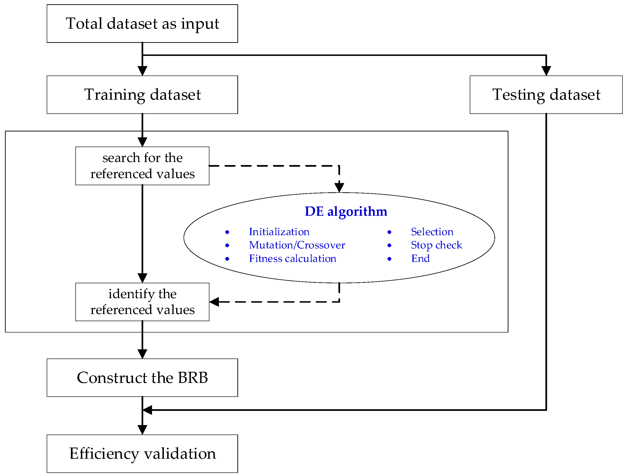
By adopting the DE algorithm as the optimization engine, the EO-BRB approach (see Figure 1) with six steps is proposed as follows:
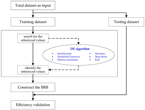
Figure 1.
Framework of the EO-BRB approach.
- Step 1: Divide the initial dataset into the training dataset and the testing dataset;
- Step 2: Determine the parameters for further optimization, and modify the DE algorithm to fit the needs of specific requirements;
- Step 3: Calculate the MSE of the training dataset;
- Step 4: Identify the best trained model with the smallest MSE;
- Step 5: Construct the new BRB system using the identified parameters including the key referenced values of the attributes;
- Step 6: Calculate the MSE of the testing dataset for efficiency validation.
3.2. The Optimization Model
The output of the ER algorithm as in Equation (14) is in the same belief structure as that of the input rules.
Consider that the utility of the nth scale u(Dn) [22], and then the numerical inference output can be calculated by Equation (15)
Since MSE is used to measure the difference between the actual output, , and the inference output, , the MSE can be modeled as in Equation (16),
where T denotes the size of the dataset. Note that the MSE function is also the optimization objective function in the DE algorithm.
With the consideration of the parameters to be optimized and the MSE model as in Equation (16), the objective function of the optimization model is given as in Equation (17) and the restraints are given in Equations (18)–(22):
s. t.
where Equation (18) describes that the referenced values should be bounded by the lower and upper bounds of the mth attribute, lbm and ubm. Equations (19) and (20) describe that, among all K rules, the minimum/maximum of the referenced rules of the ith attribute should be the lower/upper bound of the ith attribute. Equation (21) describes that the initial weight of any rule, θk, should be within the range of 0–1. Equation (22) describes that the belief of any scale in any rule, βn,k, should be within the range of 0–1.
3.3. The Optimization Algorithm
As an effective EA algorithm, the differential evolutionary (DE) algorithm is used as the optimization engine for solving the constructed optimization model in Section 3.2. The DE algorithm was first proposed to solve the Chebyshev problem. Then, it was widely used because of the simple mechanism and the high quality of the optimization results [28]. In this study, the classical DE (still referred to as DE) is applied with the following six steps.
- Step 1: Initialization.
In the initialization step, the initial population is generated with each individual representing a BRB. Moreover, the parameters are also determined, including the number of the individuals, the number of the generations, etc.
- Step 2: Mutation/Crossover.
The mutation step aims to generate new individuals. The mutation for an individual xi in the population {xi, I = 1, …, NP} is shown in Equation (23)
where, , and are three different individuals, F = 0.5 is an appropriate choice.
In the crossover step, two individuals exchange several genes and a new individual is generated, as shown in Equation (24).
where r is a random number between 0 and 1. CR ∈ [0, 1] is the crossover probability which is used to control where the mutated value should be applied in the decision variables. Normally, CR = 0.9 is an appropriate choice.
- Step 3: Fitness calculation.
The fitness function of DE produces the objective the optimization objective. Thus, the calculation procedures of the fitness function are Equations (14)–(16) in Section 3.2.
- Step 4: Selection.
For an individual ui generated in the mutation and the crossover steps, the selected individual is determined by Equation (25):
where is the objective function and is the selected individual.
- Step 5: Stop check.
The stop criterion is the preset number of generations. If it has met the stop criterion, i.e., the maximum number of generations, then, stop and go to Step 6. If it has not met the stop criterion, then go to Step 3 for a new round of optimization.
- Step 6: Output
Produce the final output.
By repeating this process, the population is updated and the solution of the problem is optimized. When the stop criterion is met, the loop could be stopped.
4. Case Study
Three cases are studied to validate the efficiency of the EO-BRB approach. Case I is based a multi-extremal function [22]. Case II is to predict the residual life probability of the metalized film capacitor for its reliability analysis [23,24]. Case III studies the pipeline leak detection which has been studied under multiple conditions [14,15,16,17,18,19,20,21]. Since DE would inevitably bring randomness, all experiments are conducted in 30 runs. Moreover, the mean square error (MSE) is adopted as the metric for the performance evaluation for maintaining consistency with previous studies.
4.1. Case I: Multi-Extremal Function
A multi-extremal function case in Reference [22] is given as in Equation (26),
In [22], a BRB system with five rules is constructed. We apply similar settings as that of [22] by supposing that there are five scales in the consequences with the utilities as {D1, D2, D3, D4, D5} = {−0.5, 0, 0.5, 1, 1.5}. Since the DE algorithm is applied, there is no need to locate the initial BRB. The settings are that (1) BRB is still assumed with 5 rules, (2) 20 individuals, and (3) 2000 generations. The objective is to minimize the MSE between the actual and the predicted outputs. The training/testing dataset is the same as that in [22] for maintaining consistency and conducting a fair comparison of 101 sets of data which are uniformed sampled from the interval [−5, 5].
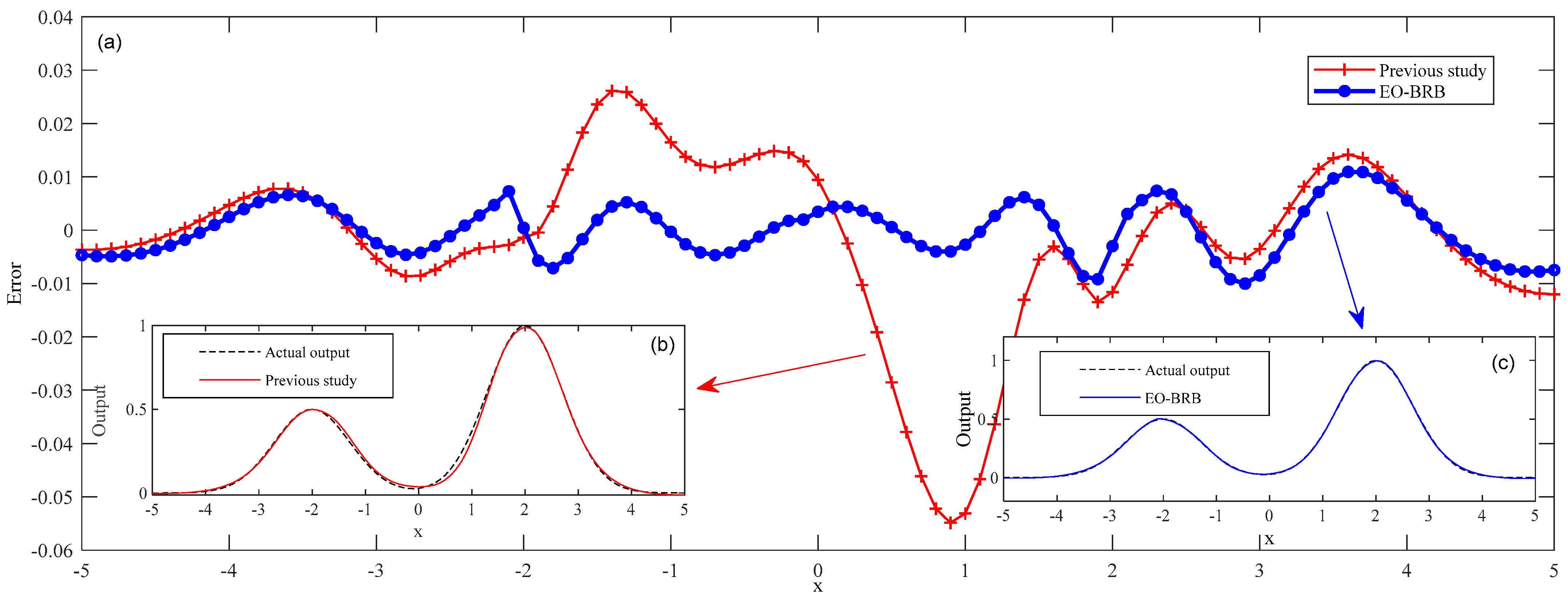
Figure 2 shows the comparison of two approaches. Table 1 shows the derived BRB. The authors in [22] calculated the MSE between the actual output and the optimized output for the 101 sets of data and it reached 6.32 × 10⁻⁵. Comparatively, the MSE between the actual output and the predicted output by the BRB in Table 1 is 2.55 × 10⁻⁵, which is 59.65% less than [22].
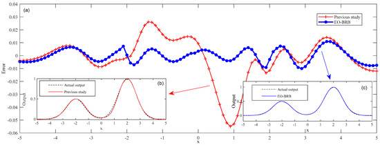
Figure 2.
Comparative results for Case I: (a) compares the errors of [22] and EO-BRB while (b) and (c) are the outputs of [22] and EO-BRB, respectively.

Table 1.
BRB with five rules for Case I.
4.2. Case II: Residual Life Probability Prediction for the Metalized Film Capacitor
The metallized film capacitors (MFCs) are critical parts of the inertial confinement fusion device which uses the high-power laser for the thermonuclear fusion under laboratory conditions [33]. It is necessary to conduct the reliability evaluation of MFC to make maintenance policies for the energy systems as well as for the high-power laser devices themselves, which in essence is to predict the MFC’s residual life or the residual life probability. For each 100 s, the residual life probability is predicted using a deduction process with the consideration of all influential factors at that time. Ref. [24] proposed a generic process to model this deduction process and predict the residual life probability of MFC, which derived the residual life probability inverse-Gauss function as in Equation (27).
where l =245, μ = 0.0001195, and σ = 0.0057. The MSE between the real-time probability and the predicted probability is 1.31 × 10⁻².
To apply the EO-BRB approach, the settings are that (1) the BRB is with 5 rules, (2) 20 individuals, and (3) 2000 generations. A total of 250 sets of data (which is half of the total dataset) are used as the training dataset and the total dataset is used as the testing dataset, which is the same as the prior study [24] for maintaining consistency and conducting a fair comparison. Additionally, suppose that there are five scales in the consequences with the utilities as {D1, D2, D3, D4, D5} = {0, 2, 4, 6, 8}.
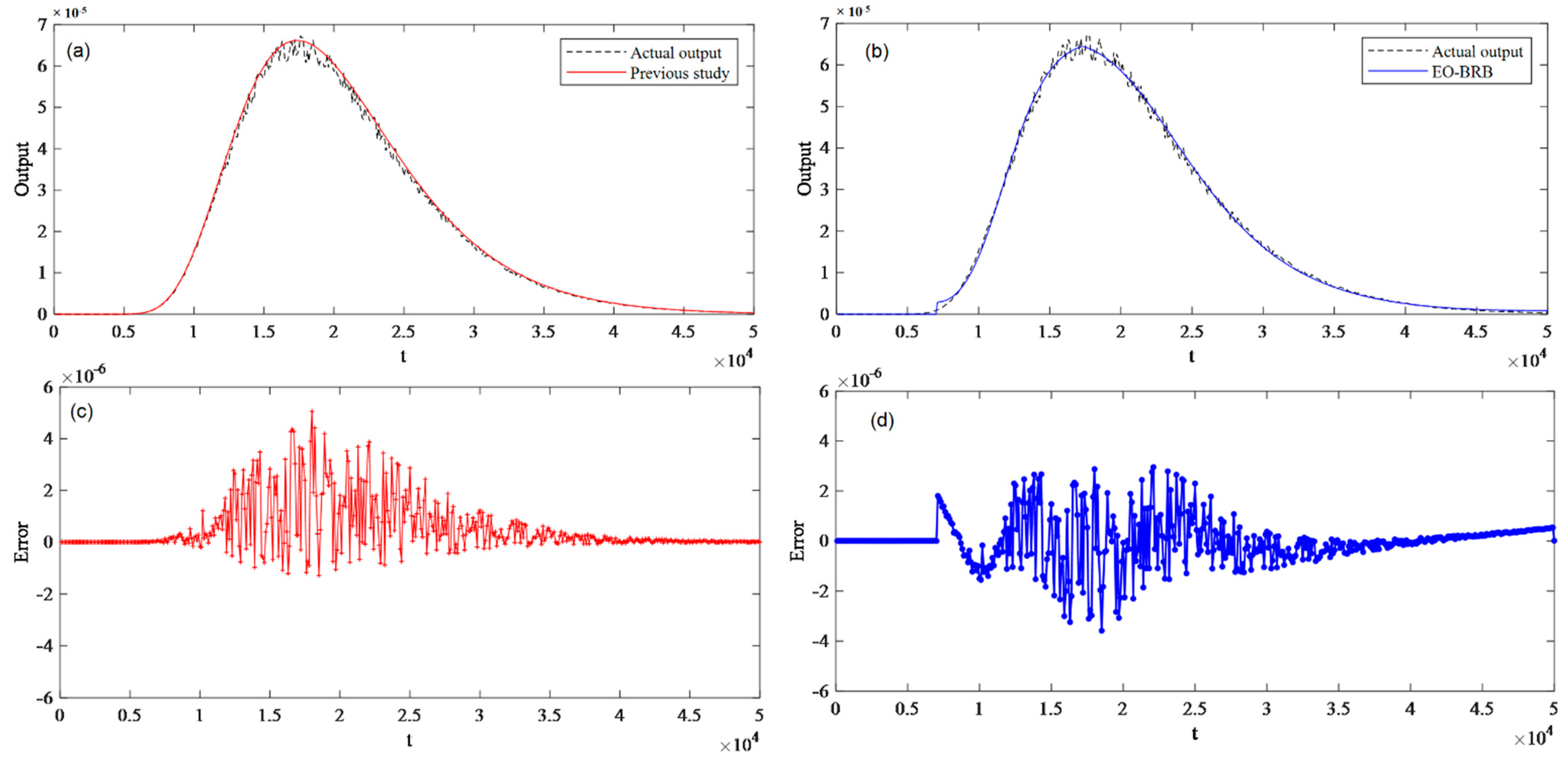
After using the EO-BRB approach, a BRB with five rules are constructed, as presented in Table 2. Furthermore, upon observing the BRB with five rules in Table 2, it is found that the last rule could be combined with the first rule and the BRB with four rules is derived as in Table 2. It is obvious that the BRBs in Table 2 are and Table 3 equivalent. Consequently, the BRB in Table 3 reaches the MSE of 9.09 × 10⁻³. Compared with the MSE = 1.31 × 10−2 by [24], the MSE by the BRB with four rules is 30.42% less. Figure 3 shows the comparison of two approaches.
Table 2.
BRB with five rules for Case II.
Table 3.
BRB with four rules for Case II.
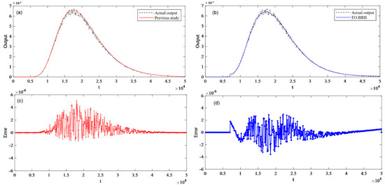
Figure 3.
Comparative results for Case II: (a,b) give outputs of the previous study and EO-BRB while (c,d) give the errors.
4.3. Case III: Pipeline Leak Detection
4.3.1. Background
The pipeline leak detection case has been extensively studied [14,15,16,17,18,19,20,21] where two factors, namely PressureDiff and Flowdiff, were used to predict pipeline leaksize. Of all the previous studies regarding on the pipeline leak detection case, there are two basic scenarios. For Scenario I, 500 sets of the total dataset is taken as the training dataset while the total dataset is taken as the testing dataset. This training/testing datasets division is the same as in [14,15,16,17,18]. For Scenario II, it is specifically based on [19,20,21] where a partial of 322 sets of data were selected from the total dataset. Of the selected 322 sets of data, the first 305 sets of data were used as the training dataset and the remaining 17 sets of data as the testing dataset. However, we do not have the same dataset of 322 sets of data as [19,20,21]. In this scenario, we select six datasets with the starting points ranging from 650th to 900th of the total dataset, and the next 17 sets of data are used as the testing dataset. Be reminded again that the training/testing datasets division in Scenarios I/II is the same as in prior studies for maintaining consistency and conducting a fair comparison.
4.3.2. Scenario I
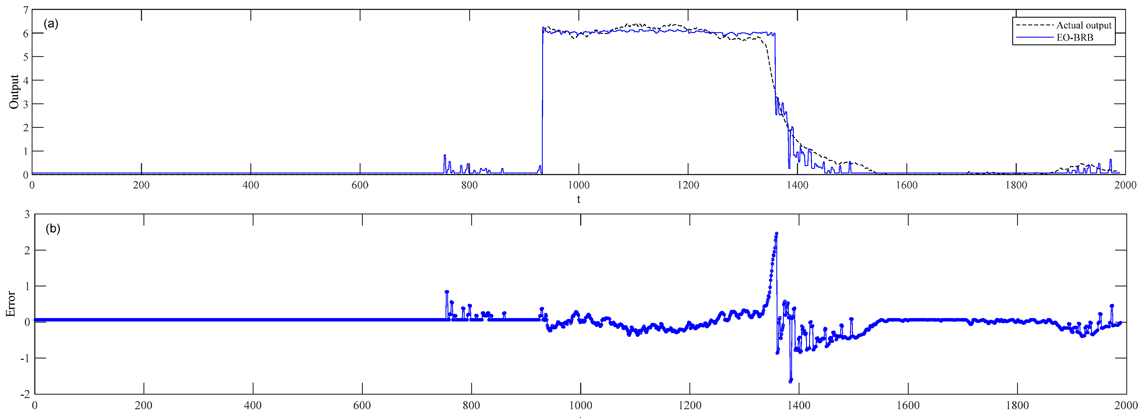
In previous studies, 500 sets of data were randomly selected from the total dataset as the training dataset (compared with 500 sets of data in [14,15] and 800/900 sets of data in [16,17,18] from a specific time interval). The total dataset is used as the testing dataset. To maintain consistency, the settings for EO-BRB are that: (1) BRB is assumed with 3 rules, (2) 20 individuals, and (3) 500 generations, whilst (4) 5 scales are assumed for leaksize as the output of BRB with the utilities as {D1, D2, D3, D4, D5} = {−3, 0, 3, 6, 9}.
The derived BRB is shown in Table 3, and Figure 4 shows the actual/predicted output/error. The MSE of the BRB as in Table 4 reaches 5.49 × 10⁻² which is far smaller than 7.78 × 10⁻¹ in [16] as it is the best result to date. Additionally, the MAE of the BRB system as in Table 4 reaches 1.35 × 10⁻¹ which is also small than 2.06 × 10⁻¹ in [15].
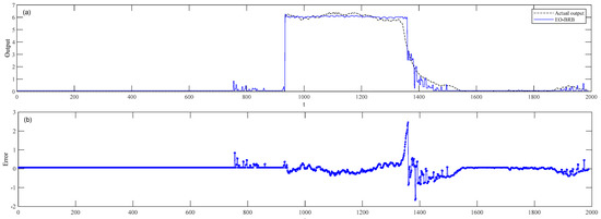
Figure 4.
Comparative results for Case III in Scenario I: (a) and (b) give the outputs and errors of EO-BRB, respectively.
Table 4.
BRB with three rules for Scenario I of Case III.
4.3.3. Scenario II
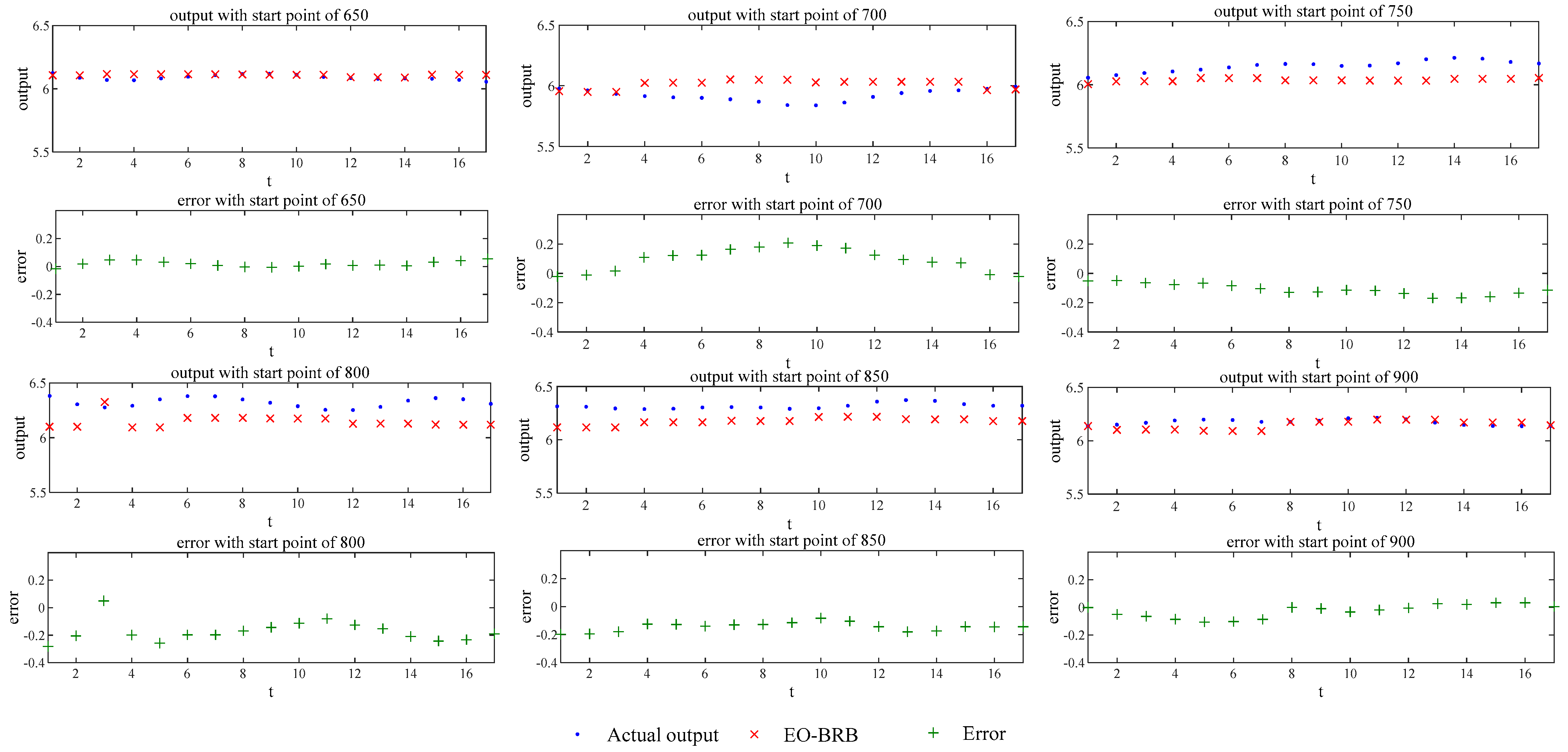
Scenario II is based on [19,20,21], where 322 sets of data were selected from the total dataset among which the first 305 sets of data become the training dataset and the rest 17 sets of data become the testing dataset. To execute a fair comparison with [19,20,21], we selected six independent datasets with similar settings. These datasets are of 322 sets of data which are selected with the start points of the 650th, 700th, 750th, 800th, 850th, and 900th in the total dataset, respectively. The settings are that (1) the BRB is with 3 rules, (2) 20 individuals, and (3) 500 generations. Table 5, Table 6, Table 7, Table 8, Table 9 and Table 10 shows the corresponding BRBs. Figure 5 shows the actual/predicted outputs and the errors of the EO-BRB approach. The errors in the six settings are 7.42 × 10⁻⁴, 1.45 × 10⁻², 1.34 × 10⁻², 3.54 × 10⁻², 2.16 × 10⁻², and 2.79 × 10⁻³, respectively. In other words, there is an improvement of 38.84% since the average MSE of six settings is 1.47 × 10⁻² by EO-BRB compared with 2.41 × 10⁻² in [19].
Table 5.
BRB with three rules for Scenario II of Case III: start point 650.
Table 6.
BRB with three rules for Scenario II of Case III: start point 700.
Table 7.
BRB with three rules for Scenario II of Case III: start point 750.
Table 8.
BRB with three rules for Scenario II of Case III: start point 800.
Table 9.
BRB with three rules for Scenario II of Case III: start point 850.
Table 10.
BRB with three rules for Scenario II of Case III: start point 900.
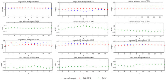
Figure 5.
Comparative results for Case III/Scenario II with different starting points.
4.4. Summary of Results and Discussion
Table 11 summarizes the statistics of traditional studies and this study. For most cases and scenarios, the number of rules and the number of the parameters to be optimized are reduced (especially in Case 3). More importantly, MSEs in these cases/scenarios are reduced as well, which validates the efficiency of the EO-BRB approach.
Table 11.
Statistics on the efficiency of the EO-BRB approach.
Table 12 further explores the efficiency of DE as the optimization engine. It shows that the variances of the MSEs in 30 runs of all cases/scenarios are far smaller compared with the average/median of MSEs. It shows that there are very stable results using DE, which further proves the validity of the application of the DE algorithm.
Table 12.
Statistics on the efficiency of the application of the DE algorithm.
According to the results in Table 11 and Table 12, there are many advantages to the proposed EO-BRB approach. (1) First, EO-BRB can effectively improve the accuracy of BRB in multiple numerical and practical conditions. (2) Moreover, only 3–5 rules are assumed in BRBs in Cases I–III, which is very cost-effective compared with other approaches that may require many more parameters. Admittedly, there are also challenges that still need to be addressed. (1) The primary concern is overfitting. Although only 3–5 rules are assumed in BRBs in this study, more rules can be used for improving the accuracy of BRB which, however, could result in overfitting. (2) Performance of EO-BRB may be affected by the selected evolutionary algorithm. Therefore, it is a challenging task to determine the optimization engine as well as its related parameters.
5. Conclusions
The EO-BRB approach is proposed by identifying the most representative referenced values of the attributes. Comparatively, the traditional learning approaches focus more on better approximating the practical systems, which contributes as the main difference between the proposed EO-BRB approach and the traditional learning approaches. Besides, the EO-BRB approach uses the DE algorithm as the optimization engine. Case study results validate the efficiency of the EO-BRB approach:
- (1)
- No need to transform numerical values into linguistic terms. The inclusion of the referenced values of the attributes as the parameters to be optimized makes the transformation process unnecessary. In addition, the DE algorithm is very effective in dealing with continuous parameters (and can also be adapted to deal with discretized parameters). Therefore, there is no need to transform numerical values into linguistic terms, which is a common step in traditional approaches. Without this transformation, the EO-BRB approach is less prejudicial from human intervention.
- (2)
- No need to pre-determine the initial solution. The DE algorithm has been proven to be very effective in finding a global optimal solution with randomly generated initial solutions. Comparatively, the traditional approaches need to pre-determine the initial solution based on certain information from the initial dataset.
- (3)
- No need for a complicated mathematical deduction process. The evolutionary mechanism in finding the optimal solution is inherited within DE, which means that this approach is universal and general. There is no need to calculate the ladder direction and/or the derivative function which are required by a traditional learning approach.
- (4)
- Furthermore, EO-BRB can help downsize the BRB system while still preserving excellent approximation with practical system. The results of three case studies show that not only the BRB systems are downsized or at least maintained as the same size, but also even smaller MSEs than the results in existed literatures are achieved.
For future work, two directions are worthy of paying attention to. Other variants of the DE algorithm or other evolutionary algorithms (GA, PSO, ACO, etc.) may be a better choice for other application cases. However, this is not the main topic of this study and is worthy of more effort. Another direction is to test on more benchmarks. The cases in this paper, especially the pipeline leak detection case, are chosen because they have been studied in the literature regarding on the learning frameworks and approaches for the BRB system. Then, more benchmark cases from other backgrounds should be further studied because only in this way can the EO-BRB approach be improved.
Author Contributions
Writing—original draft preparation, L.C. and F.S.; writing—review and editing, Z.Q. and L.C.; supervision, L.C.; programming, Z.Q., X.X. and F.S.; validation, Z.Q., F.S., X.X. and J.F. All authors have read and agreed to the published version of the manuscript.
Funding
This work was supported by the Funding of State Key Laboratory of Complex Eletromagnetic Environment Effects on Electronics and Information System (CEMEE2022Z0301B), the National Natural Science Foundation of China (Grant No. 61903108, 52171352), Zhejiang Province Key R&D projects (2021C03142), National Natural Science Foundation of Zhejiang Province (Grant No. LY21F030011), and Zhejiang Province Public Welfare Technology Application Research Projects (LGF21F020013).
Institutional Review Board Statement
Not applicable.
Informed Consent Statement
Not applicable.
Data Availability Statement
Data are available upon on request.
Acknowledgments
The authors gratefully thank Xiaobin Xu from the School of Automation, Hangzhou Dianzi University, for providing constructive suggestions.
Conflicts of Interest
The authors declare no conflict of interest.
References
- Yang, J.B.; Liu, J.; Wang, J.; Sii, H.S.; Wang, H.W. Belief rule-base inference methodology using the evidential reasoning approach-RIMER. IEEE Trans. Syst. Man Cybern. Syst. Hum. 2006, 36, 266–285. [Google Scholar] [CrossRef]
- Zhou, Z.J.; Hu, G.Y.; Hu, C.H.; Wen, C.L.; Chang, L.L. A Survey of Belief Rule-Base Expert System. IEEE Trans. Syst. Man Cybern. Syst. 2019, 51, 4944–4958. [Google Scholar] [CrossRef]
- Chang, L.; Zhang, L.; Fu, C.; Chen, Y.W. Transparent digital twin for output control using belief rule base. IEEE Trans. Cybern. 2021, 2021, 1–15. [Google Scholar] [CrossRef] [PubMed]
- Sen, M.K.; Dutta, S.; Kabir, G. Development of flood resilience framework for housing infrastructure system: Integration of best-worst method with evidence theory. J. Clean. Prod. 2021, 290, 125197. [Google Scholar] [CrossRef]
- Yang, J.B.; Xu, D.L. Evidential Reasoning rule for evidence combination. Artif. Intell. 2013, 205, 1–29. [Google Scholar] [CrossRef]
- Chang, L.; Zhang, L.; Xu, X. Correlation-oriented complex system structural risk assessment using Copula and belief rule base. Inf. Sci. 2021, 564, 220–236. [Google Scholar] [CrossRef]
- Fu, C.; Hou, B.; Xue, M.; Chang, L.; Liu, W. Extended Belief Rule-Based System with Accurate Rule Weights and Efficient Rule Activation for Diagnosis of Thyroid Nodules. IEEE Trans. Syst. Man Cybern. Syst. 2022, 2022, 1–13. [Google Scholar] [CrossRef]
- Dymova, L.; Kaczmarek, K.; Sevastjanov, P. An extension of rule base evidential reasoning in the interval-valued intuitionistic fuzzy setting applied to the type 2 diabetes diagnostic. Expert Syst. Appl. 2022, 201, 117100. [Google Scholar] [CrossRef]
- Cao, Y.; Zhou, Z.J.; Hu, C.H.; Tang, S.W.; Wang, J. A new approximate belief rule base expert system for complex system modelling. Decis. Support Syst. 2021, 150, 113558. [Google Scholar] [CrossRef]
- Zhao, D.; Zhou, Z.; Tang, S.; Cao, Y.; Wang, J.; Zhang, P.; Zhang, Y. Online estimation of satellite lithium-ion battery capacity based on approximate belief rule base and hidden Markov model. Energy 2022, 256, 124632. [Google Scholar] [CrossRef]
- Jia, Q.; Hu, J.; Zhang, W. A fault detection method for FADS system based on interval-valued neutrosophic sets, belief rule base, and DS evidence reasoning. Aerosp. Sci. Technol. 2021, 114, 106758. [Google Scholar] [CrossRef]
- Chang, L.L.; Zhou, Y.; Jiang, J.; Li, M.J.; Zhang, X.H. Structure learning for belief rule base expert system: A comparative study. Knowl. Based Syst. 2013, 39, 159–172. [Google Scholar] [CrossRef]
- Yang, J.B.; Liu, J.; Xu, D.L.; Wang, J.; Wang, Y.M. Optimization models for training belief-rule-based systems. IEEE Trans. Syst. Man Cybern. A Syst. Hum. 2007, 37, 569–585. [Google Scholar] [CrossRef]
- Zhu, H.; Xiao, M.; Yang, L.; Tang, X.; Liang, Y.; Li, J. A minimum centre distance rule activation method for extended belief rule-based classification systems. Appl. Soft Comput. 2020, 91, 106214. [Google Scholar] [CrossRef]
- Chen, Y.W.; Yang, J.B.; Xu, D.L.; Zhou, Z.J.; Tang, D.W. Inference analysis and adaptive training for belief rule based systems. Expert Syst. Appl. 2011, 38, 12845–12860. [Google Scholar] [CrossRef]
- Diao, H.; Lu, Y.; Deng, A.; Zou, L.; Li, X.; Pedrycz, W. Convolutional rule inference network based on belief rule-based system using an evidential reasoning approach. Knowl. Based Syst. 2022, 237, 107713. [Google Scholar] [CrossRef]
- Yang, L.H.; Wang, S.; Ye, F.F.; Liu, J.; Wang, Y.M.; Hu, H. Environmental investment prediction using extended belief rule-based system and evidential reasoning rule. J. Clean. Prod. 2021, 289, 125661. [Google Scholar] [CrossRef]
- Zhenjie, Z.; Xiaobin, X.; Peng, C.; Xudong, W.; Xiaojian, X.; Guodong, W. A novel nonlinear causal inference approach using vector-based belief rule base. Int. J. Intell. Syst. 2021, 36, 5005–5027. [Google Scholar] [CrossRef]
- Zhou, Y.; Chang, L.; Qian, B. A belief-rule-based model for information fusion with insufficient multi-sensor data and domain knowledge using evolutionary algorithms with operator recommendations. Soft Comput. 2019, 23, 5129–5142. [Google Scholar] [CrossRef]
- Kabir, S.; Islam, R.U.; Hossain, M.S.; Andersson, K. An integrated approach of belief rule base and deep learning to predict air pollution. Sensors 2020, 20, 1956. [Google Scholar] [CrossRef]
- Xu, X.; Zhao, Z.; Xu, X.; Yang, J.; Chang, L.; Yan, X.; Wang, G. Machine learning-based wear fault diagnosis for marine diesel engine by fusing multiple data-driven models. Knowl. Based Syst. 2020, 190, 105324. [Google Scholar] [CrossRef]
- Chen, Y.W.; Yang, J.B.; Xu, D.L.; Yang, S.L. On the inference and approximation properties of belief rule based systems. Inf. Sci. 2013, 234, 121–135. [Google Scholar] [CrossRef]
- Wang, X.L.; Guo, B.; Cheng, Z.J. Residual life estimation based on bivariate Wiener degradation process with time-scale transformations. J. Stat. Comput. Sim. 2014, 84, 545–563. [Google Scholar] [CrossRef]
- Liu, S.; Zhang, J.; Zhang, Z. Lifetime Prediction of Mica Paper Capacitors Based on an Improved Iterative Grey-Markov Chain Model. IEEE J. Emerg. Sel. Top. Power Electron. 2022, 2022, 1. [Google Scholar] [CrossRef]
- Srorn, R.; Price, K. Differential Evolution—A Simple and Efficient Heuristic for Global Optimization over Continuous Spaces. J. Glob. Optim. 1997, 11, 341–359. [Google Scholar]
- Yang, J.Q.; Chen, C.H.; Li, J.Y.; Liu, D.; Li, T.; Zhan, Z.H. Compressed-Encoding Particle Swarm Optimization with Fuzzy Learning for Large-Scale Feature Selection. Symmetry 2022, 14, 1142. [Google Scholar] [CrossRef]
- Fu, B.J.; Zhang, J.P.; Li, W.J.; Zhang, M.J.; He, Y.; Mao, Q.J. A Differential Evolutionary Influence Maximization Algorithm Based on Network Discreteness. Symmetry 2022, 14, 1397. [Google Scholar] [CrossRef]
- Das, S.; Suganthan, P.N. Differential Evolution: A survey of the state-of-the-art. IEEE Trans. Evol. Comput. 2011, 15, 4–31. [Google Scholar] [CrossRef]
- Lv, C.; Liu, J.; Zhang, Y.; Lei, W.; Cao, R.; Lv, G. Reliability modeling for metallized film capacitors based on time-varying stress mission profile and aging of ESR. IEEE J. Emerg. Sel. Top. Power Electron. 2020, 9, 4311–4319. [Google Scholar] [CrossRef]
- Mirjalili, S. Evolutionary Algorithms and Neural Networks. Studies in Computational Intelligence; Springer: Berlin/Heidelberg, Germany, 2019; p. 780. [Google Scholar]
- Bui, D.T.; Panahi, M.; Shahabi, H.; Singh, V.P.; Shirzadi, A.; Chapi, K.; Ahmad, B.B. Novel hybrid evolutionary algorithms for spatial prediction of floods. Sci. Rep. 2018, 8, 15364. [Google Scholar] [CrossRef]
- Fu, C.; Xu, C.; Xue, M.; Liu, W.; Yang, S. Data-driven decision making based on evidential reasoning approach and machine learning algorithms. Appl. Soft Comput. 2021, 110, 107622. [Google Scholar] [CrossRef]
- Belko, V.O.; Emelyanov, O.A.; Ivanov, I.O.; Plotnikov, A.P. Self-Healing Processes of Metallized Film Capacitors in Overload Modes—Part 1: Experimental Observations. IEEE Trans. Plasma Sci. 2021, 49, 1580–1587. [Google Scholar] [CrossRef]
Publisher’s Note: MDPI stays neutral with regard to jurisdictional claims in published maps and institutional affiliations. |
© 2022 by the authors. Licensee MDPI, Basel, Switzerland. This article is an open access article distributed under the terms and conditions of the Creative Commons Attribution (CC BY) license (https://creativecommons.org/licenses/by/4.0/).