Circuit Complexity from Supersymmetric Quantum Field Theory with Morse Function

Abstract

Computation of circuit complexity has gained much attention in the theoretical physics community in recent times, to gain insights into the chaotic features and random fluctuations of fields in the quantum regime. Recent studies of circuit complexity take inspiration from Nielsen’s geometric approach, which is based on the idea of optimal quantum control in which a cost function is introduced for the various possible path to determine the optimum circuit. In this paper, we study the relationship between the circuit complexity and Morse theory within the framework of algebraic topology, which will then help us study circuit complexity in supersymmetric quantum field theory describing both simple and inverted harmonic oscillators up to higher orders of quantum corrections. We will restrict ourselves to $\mathcal{N}=1$ supersymmetry with one fermionic generator $Q_{\alpha }$. The expression of circuit complexity in quantum regime would then be given by the Hessian of the Morse function in supersymmetric quantum field theory. We also provide technical proof of the well known universal connecting relation between quantum chaos and circuit complexity of the supersymmetric quantum field theories, using the general description of Morse theory.

1. Introduction

AdS/CFT correspondence has helped in providing great insights on the geometry of the bulk from information in the boundary CFT [1,2,3,4,5,6]. In essence, it means that, given a conformal field theory is holographic and it has a dual theory in classical gravity, then the states of these CFTs are associated with a certain state of the dual theory: an empty vacuum corresponds to a pure AdS, a thermal state on $S^d$ to a Schwarzschild Black hole etc. The Ryu–Takayanagi formula interprets the entropy of any CFT substate, for a CFT with a gravitational dual. Generalizations of the formula [7,8,9,10] have been used in various descriptions to study bulk aspects of gravitational systems especially black-holes using holographic entanglement and information of the boundary CFT [11,12,13,14,15]. However, probing the physics behind the horizon is still a major challenge. It has been inspected that, even if the entangled entropy of an eternal AdS black hole saturates after reaching the equilibrium, the size of the Einstein–Rosen (ER) bridge continues to grow with time, posing a problem to the dual description of boundary CFT. Considering this, Susskind has introduced new observables in bulk geometry [16,17,18,19,20,21,22]. These new observables are measures of quantum information that assist in further probing the wormhole [23]. One is the volume of a maximal co-dimension-one bulk surface extending to the boundary of AdS space-time, and the second is the action defined on the Wheeler–DeWitt patch. According to the conjecture, these new observables are a dual description of the complexity of the boundary field theory.

One of these crucial observables is volume, which according to the “Complexity = Volume” conjecture, states that the volume $\mathcal{V}\left(\mathcal{B}\right)$ of a maximal co-dimension-one bulk surface $\mathcal{B}$ that extends to the AdS boundary and asymptotic to the time slice ∑ is proportional to the complexity of the boundary state, $C_{\mathcal{V}}\left(\sum \right)$, which is given by:

$$C_{\mathcal{V}}\left(\sum \right)=max\left[\frac{\mathcal{V}\left(\mathcal{B}\right)}{G_{N}l}\right].$$

(1)

The second observable is the gravitational action estimated in the Wheeler–DeWitt (WDW) patch in the bulk region ${\mathcal{I}}_{WDW}$, which according to the another important conjecture, namely the “Complexity = Action” conjecture, is proportional to complexity of the boundary field theory [24], given by:

$$C_A=\frac{{\mathcal{I}}_{WDW}}{\pi \hslash }.$$

(2)

Complexity in quantum field theory and various other quantum systems has been the attraction of the theoretical physics community in recent times. The growth of quantum complexity in many systems and similar behavior inside black holes has given insights about what happens inside the horizon of a gravitational dual and helps understanding it in terms of entanglement of the boundary fields [25,26]. Recent works have shown that the ambiguities in formulation of quantum complexity (such as the choice of operations/gates) is highly sensitive and a class of these observables exist and can be used to study information theoretic properties of the bulk and even relate it to the classical entropy as their growth rates are very similar [23,27]. Circuit complexity has been used in the context of many field theories in recent times to study decaying and scattering phenomenon outside equilibrium [28,29,30,31]. In other words, it helps in understanding the out-of-time-order-correlation (OTOC) function of observables in a quantum system that depicts the chaotic and random quantum fields [32,33,34]. OTOC within the framework of supersymmetric quantum mechanics was studied in the simple harmonic oscillator, one dimensional infinite potential well and various other models in [35,36]. The main idea was to put the free scalar field theory on a lattice, which reduces it to a family of coupled oscillators, then identifying the circuit as a path-ordered exponential of Hamiltonian, which forms the representation of $GL(2,R)$, and then constructing the Euclidean metric. Minimizing the length of this metric would finally give the expression for circuit complexity. These results were obtained in the inverted harmonic oscillator framework and interacting field theories to look for chaotic behavior in quantum field theories (QFT). In this paper, our main objective is to calculate circuit complexity for supersymmetric quantum field theories for simple and inverted harmonic oscillators for various higher-order quantum corrections. We will restrict ourselves to $\mathcal{N}=1$ supersymmetry, such that we will have only one fermionic annihilation and creation operator and thereby only one supercharge. We will take an unusual approach and first try to connect complexity in quantum field theories, namely, supersymmetric field theories, with the Morse function. Morse theory acts as an essential tool to study the topology of manifolds by studying the differentiable functions through which we could identify the critical points on that manifold: the minima, maxima, and saddle points. To study the connection between circuit complexity in supersymmetric quantum field theories with the Morse function, we will first identify the so-called “cost function", an important parameter in computing the circuit complexity. The cost function counts the number of gates operating at a particular time t to construct the optimal circuit with the Morse function on a given manifold. By computing the Hessian of the Morse function, we obtain the expression for circuit complexity in the present context of the discussion. Our motivation for doing so lies in the fact that the eigenvalues of supersymmetric Hamiltonian are closely concentrated near the Morse function’s critical points. The number of zero eigenvalues of the ground state is exactly equal to the Betti number of the manifold. In this paper, we will show how the increase in the number of critical points of the manifold captures the amount of chaos present in supersymmetric quantum field theories for the inverted harmonic oscillator (IHO) and how the mathematical structure of supersymmetry (SUSY) in the regime inverted harmonic oscillators whose potentials forms the generators of SL(2, R) group underlies chaos. It makes the number of critical points increase by a factor of an exponential with respect to the superpotential appearing in supersymmetric quantum field theory. For the scalar field theories in the regime where it can be described as a simple harmonic oscillator (SHO), we will identify the non-dynamical auxiliary field; namely the F-term in the Lagrangian of SUSY theory involving scalar fields; with the gradient of the Morse function, which passes through every critical point on the manifold. In turn, we will show that the complexity of supersymmetric quantum field theories for simple harmonic oscillator only depends on the absolute value of the non-dynamical auxiliary field, which also acts as an order parameter for supersymmetry breaking. This way of identifying the F-term with the gradient of the Morse function provides another way to check when the supersymmetry is broken. If the gradient flow passes through the critical points, then it could be said that there exist no ground states with zero energy or SUSY is spontaneously broken. Following this, we will compute the Hessian in the space of super-coordinates and will derive the expression for complexity. Edward Witten has shown that supersymmetric quantum field theory is a Hodge Derham cohomology and has derived the Morse inequality using the formalism of supersymmetry. This paper will not work along the same lines, but our main objective would be to give quantum chaos a topological flavor in supersymmetric theories. At present, the Out-of-time ordered correlation (OTOC) function has been an essential theoretical tool to capture the effect of chaos in any quantum system at late time scales. By following this fundamental notion, in this paper, we will explicitly give a technical proof of the universal relation relating circuit complexity with the quantum chaos in terms of the previously mentioned Out-of-Time Ordered Correlation Function (OTOC) within the framework of the supersymmetric quantum field by using the general description of Morse theory.

Organization of the paper is as follows:

• In Section 2, we provide a brief review of the concept of circuit complexity in the general context of quantum information theory.
• In Section 3, we will explain the Lie algebra formulation and how the potential of the Inverted Harmonic Oscillator (IHO) could be embedded in the structure of the manifold.
• In Section 4, we will give a brief review of Morse theory, namely the Morse function and the gradient flow of the Morse function for completeness.
• In Section 5, we will comment on the relationship between circuit complexity and Morse function over a manifold in supersymmetric quantum mechanics.
• In Section 6, we will explicitly compute the expression of circuit complexity for the Inverted Harmonic Oscillator (IHO) up to higher-order of quantum corrections.
• In Section 7, we will compute the complexity for supersymmetric field theories for simple harmonic oscillators up to higher orders of quantum corrections in terms of the non-dynamical auxiliary field. We will compare the results of complexity between supersymmetric and non-supersymmetric quantum field theory for SHO and IHO in

  Table 1. Comparison in circuit complexity between SUSY & NON-SUSY QFT for SHO.

  Parameter	Non-SUSY QFT		SUSY QFT
  -	${\mathit{\varphi }}^{\mathbf{4}}\mathbf{+}{\mathit{\varphi }}^{\mathbf{2}}$	${\mathit{\varphi }}^{\mathbf{2}}$	${\mathit{\varphi }}^{\mathbf{4}}\mathbf{+}{\mathit{\varphi }}^{\mathbf{2}}$	${\mathit{\varphi }}^{\mathbf{2}}$
  Mass	Complexity for non-supersymmetric field theories has polynomial as well as logarithmic dependence on the mass parameter as $log\left(m\delta \right)$	Circuit complexity for Non-SUSY QFT has logarithmic support on the square of the mass parameter $log\left(m^2\delta \right)$, and in the infrared (IR) region it takes the form $-lo{g}^k\left(mk\right)$.	Complexity for supersymmetric field theories has only polynomial dependence, namely the quadratic exponent of the mass parameter. For large masses we observe a decrease in rate and reaches a saturation value.	Complexity for supersymmetric field theories in case of quadratic perturbations also has polynomial, namely quadratic, dependence on the mass parameter.
  Topological dependence	Complexity for non-supersymmetric field theories has a fractional reliance on the volume of lattice for interacting terms, such as $V^{\frac{1}{2}}$ for dimension $d=3$	Complexity due to just quadratic perturbations in Non-SUSY QFT does not have any topological dependence but depends on the dimension of lattice used for computations	Complexity for supersymmetric field theories due to quadratic interactions depends on the Hessian of the Morse function whose gradient has been identified with the auxiliary field and also on the critical points of the manifold and hence has topological dependence	SUSY complexity due to quadratic term in the superpotential also depends on topological parameters (Hessian of the Morse function) defined on the manifold.
  Dependence on the field	Complexity for non-supersymmetric field theories depends on various parameters of a quantized field in theories and the strength of interaction with each other and normal frequency modes	Due to quadratic perturbations, complexity for Non-SUSY field theories on a lattice depends on components of the momentum vectors and the number of oscillators in the lattice formalism. It does not depend on the coupling parameter.	Complexity for SUSY QFT only depends on the absolute value of the non-dynamical auxiliary field, namely the $F-term$ as $F=\frac{m\varphi +\lambda {\varphi }^3}{2}$ which is identified as the gradient of the Morse function, which passes through every critical point on the surface	In case of quadratic perturbation complexity changes due to the shift of F-term which by solving the equation of motion is given by $\frac{m\varphi }{2}$ and does not have any dependence on coupling constant
  Growth of complexity	Complexity for perturbating term ${\varphi }^4$ for dimension $d>0$ breaks down and in the limit $\lambda \to 0$ the circuit complexity have a continuous limit	In the infrared scale i.e ${\omega }_0\ll \frac{1}{\delta }$ their is an additional logarithmic factor in the complexity and lead to divergences in the limit $\delta \to 0$.	When we change coupling $\lambda$ from 1 to −1, we observe that complexity first rises and then have a sudden dip. As we go to more negative values of lambda, we observe the rate of saturation to be faster.	In supersymmetric field theories, we have strangely observed that complexity first rapidly grows and then saturates does not change much when we change the coupling $\lambda$ to −1

  ,

  Table 2. Discussions on Lyapunov exponent for SHO complexity.

  Parameters of SHO	Features of Graph and Lyapunov
  General features	The graphs rise fast initially and then slowly saturate. The rate of saturation and complexity at the saturation point depends on the order for perturbation, with ${\varphi }^4$ term being the slowest to saturate. Hence the slope is significant, and the Lyapunov exponent is expected to be larger for ${\varphi }^4$ theory. The ${\varphi }^3$ theory saturates quickly, giving a smaller slope than the rest and a smaller Lyapunov exponent.
  Mass	For large masses we observe a decrease in rate and saturation value of ${\varphi }^4$ theory. It becomes in-differentiable to the ${\varphi }^2$ term as we approach massive fields (hence a smaller Lyapunov exponent). For smaller masses the ${\varphi }^3$ graph approaches ${\varphi }^2$, decreasing slightly in rate. We can expect a slight increment in the Lyapunov exponent.
  $\lambda$	When we make $\lambda$ negative we observe the saturation is slower in ${\varphi }^2$ and ${\varphi }^3$ perturbations. In the case of ${\varphi }^4$ perturbation, we encounter a zero, thereby right-shifting the point of initial rise, increasing the value of the Lyapunov exponent. As we go to more negative values of lambda, we observe the rate of saturation to be faster, and we expect the Lyapunov exponent to be smaller.

  and

  Table 3. Comparison in complexity between NON-SUSY & SUSY QFT for IHO.

  Parameter	Non-Supersymmetric QFT (${\mathit{\varphi }}^2$)	Supersymmetric QFT (${\mathit{\varphi }}^2$)
  Mass	Circuit complexity for Non-SUSY QFT in the regime of inverted harmonic oscillators has a quadratic dependence on a mass parameter in the exponential type function, namely the inverse cosine hyperbolic function. It has also been observed that complexity starts to increase before the critical value $\lambda =m^2$.	Circuit complexity for supersymmetric field theories for the inverted harmonic oscillator also has a quadratic dependence on the mass parameter in the exponential function. We also observe that as mass increases, the rate of change of complexity increases.
  Topological dependence	Circuit complexity of Non-supersymmetric quantum field theories does not have any topological dependence. However, it depends on the number of oscillators and dimension of the lattice	Circuit complexity for supersymmetric field theories depends on the critical points of the manifold, and for even values of $F-\gamma$, we see that complexity increases exponentially.
  $\lambda$	The complexity starts to increase for $\lambda <{\lambda }_c$. At the critical point, the complexity sharply increases. Beyond the critical value $\lambda =m^2$, the model becomes unstable. We expect the complexity to grow rapidly with decreasing pick up time	The change in the value of $\lambda$ contributes to the rate with increasing values resulting in faster rates of increase and hence higher slopes. For negative values of $\lambda$ we observe that complexity decreases exponentially, and the model becomes irrelevant.
  Growth in complexity	For inverted harmonic oscillator, complexity for non-supersymmetric field theories for the initial time is nearly zero, after which it exhibits linear growth.	On the contrary, the inverted harmonic oscillator complexity does not exhibit any exponential or linear growth, as seen in figure (5).

  .
• In Section 8, we will provide the detailed numerical and graphical analysis of the results for both SHO and IHO using the prescription of supersymmetric Morse quantum field theory.
• In Section 9, we will derive the universal relation between the circuit complexity and quantum chaos expressed in terms of OTOC function for supersymmetric quantum field theory prescription using the Morse function.
• Finally Section 10, we will conclude our result and comment on how the behavior of complexity for the supersymmetric model is already implemented in the structure of a manifold.

2. Circuit Complexity for Dummies

The notion of circuit complexity was first introduced in information theory to find the minimum number of gates to acquire the desired state from an initial state. It involves acting the initial state with a unitary operator or a set of quantum gates to obtain the desired target state.

$$|{\psi }_T\rangle =U|{\psi }_i\rangle$$

(3)

There exist many such sets of unitary operators to obtain the desired final state but to find a minimum number of such operations to execute the task is what constitutes an optimal quantum circuit. Taking inspiration from this, Nielsen and collaborators have developed this idea further and have taken a geometric approach to finding the most optimal quantum circuit to get the desired target state via unitary operations in physics [26,37,38,39,40,41,42,43,44,45,46],

$$U\left(t\right)=\mathcal{P}exp\left(-i{\int }_0^{t}H\left(t\right)dt\right)\mathrm{where}H\left(t\right)=\sum Y^I\left(t\right)M_I,$$

(4)

where $M_I$ are the Pauli matrices and $Y^I\left(t\right)$ are referred to as the control function that decides the nature of gate that will act at a certain value of parameter t. This setup is a toy model for fermionic 1 + 1 dimensional theory, for higher dimension appropriate operators and their generators are considered. Given that the left hand side is a unitary operator, the right hand side will have the particular generators $M_I$ and their coefficients $Y_I$ which are tangent velocities in the unitary operator space. This approach of identifying the action of quantum gates via control function could be modified in terms of finding the extremal curves, i.e., geodesics. Hence we define a cost function $F(U\left(t\right),\dot{U\left(t\right)})$ which is a function of the unitary operator U and a vector at a point in the tangent space formed by unitaries. The idea is to minimize this cost function for various possible paths, which is described by the following expression:

$$\mathcal{D}\left(U\left(t\right)\right)={\int }_0^1\left(F(U\left(t\right),\dot{U\left(t\right)}\right)dt$$

(5)

The task now is to determine the cost function which as described above counts the number of gates to construct the optimal quantum circuit. A general class of cost functions are:

$$F_p(U,Y)=\sum p_I\left|Y^I\right|,$$

(6)

$$F_q(U,Y)=\sqrt{\sum q_I{\left(Y^I\right)}^2},$$

(7)

where minimizing $F_2=\sqrt{\sum {\left(Y^I\left(s\right)\right)}^2}$, which is a quadratic cost functional, would give us the expression for the length of geodesic of a Riemann surface. The length of the geodesic traced out by intermediate states in constructing target state via minimum number of gates would give us an expression for complexity

$$C=\underset{Y\left(s\right)}{min}\int l\left(ds\right)=\underset{Y\left(t\right)}{min}\int dt\sqrt{{\left({\partial }_{t}Y\left(t\right)\right)}^2}.$$

(8)

The gate action on the reference state could be written in terms of the generators decided by the Hamiltonian and an arbitrary small parameter $ϵ$ as:

$$U=exp\left[M_{IJ}ϵ\right]$$

(9)

where $M_{IJ}$ are the suitable generators decided by the Hamiltonian of the model. We can choose from a class of generators that performs the Unitary operation of taking a reference state to a target state. We can then find explicit expression for the velocity $Y_I$ by rewriting Equation (4) in the following form:

$$Y_I\left(s\right)=i\left({\partial }_{s}U\left(s\right)\right)U^{-1}\left(s\right),$$

(10)

where we have used $Tr\left(M_I{M}^J\right)={\delta }_{IJ}$. The general expression for the cost function could be further written as:

$$Y^I\left(s\right)=\mathrm{Tr}[i\left({\partial }_{s}U\left(s\right)\right)\left(U^{-1}\left(s\right)M_I^T\right]$$

(11)

We have written the expression for cost function in terms of the unitary operators which will explicitly demonstrate the relation between it and the Morse function for the supersymmetric Hamiltonian $H_t$ to compute the circuit complexity for supersymmetric field theories.

3. Lie Algebra Formulation of the Inverted Harmonic Oscillator (IHO)

To work out the circuit complexity in various models researchers have considered a simple, exactly solvable system known as the Inverted Harmonic Oscillator (IHO), which is described by the Hamiltonian function:

$$H(p,x)=\frac{p^2}{2}-\frac{1}{2}{\omega }^2{x}^2.$$

(12)

This encapsulates the sensitivity to initial conditions exhibited by the chaotic systems [47,48,49]. The Inverted Harmonic Oscillator (IHO) differs from the Simple Harmonic Oscillator (SHO) in many ways. For instance, the energy spectrum of IHO has a continuous energy spectrum, whereas the regular SHO has a discrete energy spectrum $(n+\frac{1}{2})\hslash \omega$. While the SHO provides a good description of the deviations from the stable equilibrium, the IHO models the decay from an unstable equilibrium. The IHO in recent times has been proven to be incredibly useful to show the equivalence among various diverse fields. The IHO appears in the quantum hall effect and in the mechanism of the Rindler Hamiltonian, whose time evolution would give rise to the Hawking–Unruh effect [50,51,52]. The equivalence between the two phenomena can be shown in terms of the isomorphism of the underlying lie algebra [53,54].

In this paper, our main objective will not be to formally describe the Lie algebra isomorphism but instead using that to calculate the circuit complexity over a manifold via Morse function for supersymmetric quantum field theories. To do this, first we have to show how the potential of IHO forms the generators of Lie algebra. Fortunately, such a construction has already been carried out and we will briefly review it below, for details readers can refer to [48]. We start with the settings of the quantum hall effect (QHE), the three quadratic potentials generate the Hamiltonian dynamics in the lowest Landau level (LLL):

$$P_{LLL}{V}_1{P}_{LLL}=\lambda (R_x^2+R_y^2),$$

(13)

$$P_{LLL}{V}_2{P}_{LLL}=\lambda (R_X{R}_Y+R_Y{R}_Y),$$

(14)

$$P_{LLL}{V}_3{P}_{LLL}=\lambda (R_x^2-R_y^2).$$

(15)

By projecting the generators to the lowest Landau level one can find $P_{LLL}{J}_{ij}{P}_{LLL}=\frac{1}{4l_B^2}{ϵ}_{ijk}\{R_i,R_k\}+\mathcal{O}\left(1\right)$. From this we see that

$$P_{LLL}{V}_1{P}_{LLL}=\frac{-4\lambda l_B^2}{\hslash P_{LLL}L{P}_{LLL}},$$

(16)

$$P_{LLL}{V}_2{P}_{LLL}=2\lambda l_B^2{P}_{LLL}{j}_i{P}_{LLL},$$

(17)

$$P_{LLL}{V}_3{P}_{LLL}=\frac{-4\lambda l_B^2}{\hslash P_{LLL}{j}_j{P}_{LLL}}.$$

(18)

where $P_{LLL}$ is the projection operator to the lowest Landau level, $R_X,R_Y$ are bilinears and $j_a,j_b$ are strain generators. Therefore by projecting the potentials to the LLL both bilinears and the strain generators lead to the quadratic Hamiltonian which is similar to the electrostatic potential and IHO appears in quantum Hall effect as might expected.

We now rename the three quadratic potentials in a quantum Hall effect $V_1,V_2,V_3$ as $K_1,K_2,K_3$ and we identify:

$$P=\frac{R_x}{l_B},X=\frac{R_y}{l_B}.$$

(19)

Consequently from (15), we get the Hamiltonians in the LLL to be of the following form:

$$K_1=(P^2+X^2),$$

(20)

$$K_2=(PX+XP),$$

(21)

$$K_3=(P^2-X^2).$$

(22)

On the basis of LLL wave functions the potentials could be written the form of differential operators namely [48]:

$$K_1=\frac{1}{4}\left(-\frac{{\partial }^2}{\partial X^2}+X^2\right),$$

(23)

$$K_2=\frac{i}{2}\left(X\frac{\partial }{\partial x}+\frac{1}{2}\right),$$

(24)

$$K_3=\frac{1}{4}\left(-\frac{{\partial }^2}{\partial X^2}-X^2\right).$$

(25)

These are precisely the generators of $SL(2,R)$ Lie-algebra [55], which act as an area preserving deformation of a two dimensional manifold and satisfy the following non-commuting relations:

$$[K_2,K_3]=-i{K}_1,$$

(26)

$$[K_1,K_2]=i{K}_3,$$

(27)

$$[K_3,K_1]=i{K}_2.$$

(28)

With these techniques at hand, our main objective will now be to describe a Morse function on a manifold formed by the Lie-algebra of SL(2, R), namely the potential of the IHO. Then we will show how the critical points of the Morse function on a manifold play the role of the cost function, which decides the gate in action at a particular parameter t to form the optimal circuit.

4. Brief Review of Morse Theory

In this section, we are going to give a very brief review of Morse theory. The Morse function helps classify surfaces up to homeomorphism when it passes the critical point of index 0, 1, 2. The indices 2, 1, and 0 represent the maximum, minimum and saddle points of the manifold, respectively.

4.1. Definition of Morse Function

To define the Morse function [56,57] we consider a manifold $\mathcal{M}$ and a function f such that:

Theorem 1.

A smooth map $f:X^n$⟶R is a Morse function if, for every critical point p ∈ X, ∃ coordinates $x_1,\dots ,x_n$, and a coordinate y around $f\left(p\right)$ w.r.t. which,

$$f(x_1,\dots .,x_n)=-x_1^2-x_2^2-\dots .-x_k^2+x_{k+1}^2+\dots +x_n^2.$$

(29)

such that the value of the function at the critical points vanishes.

Theorem 2.

A map f ⟶ R is a Morse function if its critical points vanishes and the Hessian of f at each critical point is non-singular. A Morse function on a compact manifold X helps to determine it’s topology, by mapping its critical points to an axis on a one-dimensional plane, which helps to encode a lot of information about $\mathcal{M}$ [58]. The goal of the Morse theory is to find the invariant of the manifold by counting the critical points of chosen Morse function.

4.2. Gradient Flow of Morse Function

The gradient flow of the Morse function creates a vector field on the surface of the manifold, which helps to define a notion of transport from one point to another. Let us suppose we have an integral curve ${\gamma }_x$: $R⟶M$ such that:

$${\gamma }_x\left(t\right)={\varphi }_t\left(x\right),{\varphi }_0\left(x\right)=0.$$

(30)

Here $\varphi$ is a smooth one-parameter group of diffeomorphism on $\mathcal{M}$. Then, we get:

$$\begin{array}{ccc}\hfill \frac{d}{dt}f\left({\gamma }_x\left(t\right)\right)& =& \frac{d}{dt}(f\circ {\varphi }_t\left(x\right))\hfill \\ & =& d{f}_{{\varphi }_t\left(x\right)}\circ \frac{d}{dt}{\varphi }_t\left(x\right)\hfill \\ & =& d{f}_{{\varphi }_t\left(x\right)}(-\nabla f){\varphi }_t\left(x\right)\hfill \\ & =& -\left|\right|(\nabla f){\varphi }_t\left(x\right){\left|\right|}^2\le 0.\hfill \end{array}$$

(31)

Thus the gradient flow of f is decreasing down the lines of ${\gamma }_x$. One of the reasons we have defined the gradient flow of the Morse function will become apparent in the latter part of this paper, where it will play a crucial role in deriving the complexity of supersymmetric field theories for the SHO.

5. Circuit Complexity in SUSY QFT via Morse Function

To compute circuit complexity within the framework of supersymmetric quantum field theory using the Morse function, we will consider SL(2, R) modular curve, which encodes the potential of IHO as generators of Lie algebra and identifies it with a Riemann manifold $\mathcal{M}$, and the Morse function to the cost function as described in the previous section, and thereby associate the critical points to the action of the control function which decides, which quantum gate will be active at a particular time t.

The supersymmetric operators in terms of an exterior derivative and its adjoint can be described as:

$$Q_1=d+d^{*},$$

(32)

$$Q_2=i(d-d^{*}),$$

(33)

$$H=d{d}^{*}+d^{*}d.$$

(34)

The connection between supersymmetric quantum field theories and Derham operators could found in the Ref. [59]. Then further by taking into account the following crucial fact:

$$d^2=0=d^{*2},$$

(35)

We get the following subsequent supersymmetric relations in the present context, which are given by:

$$Q_1^2=Q_2^2=H,$$

(36)

$$Q_1{Q}_2+Q_2{Q}_1=0.$$

(37)

Now let us consider a Morse function f on the surface of the manifold M, and t be a real number. Then,

$$d_t=exp(-ht)dexp\left(ht\right),$$

(38)

$$d_t^{*}=exp(-ht)d^{*}exp\left(ht\right).$$

(39)

Here we can show that:

$$d_t^2=0=d_t^{*2},$$

(40)

Using which we get the following expressions:

$$Q_{1t}=d+d^{*},$$

(41)

$$Q_{2t}=i(d_t-d_t^{*}),$$

(42)

$$H_t=d_t{d}_t^{*}+d_t^{*}{d}_t.$$

(43)

We will now explicitly calculate the formula for $H_t$ in terms f, to understand how critical points come into the picture. Let $v^k\left(p\right)$ and $v^k*$ be an orthonormal basis of tangent vectors and the corresponding dual vectors at each point p in $\mathcal{M}$, respectively. The $a^k$ acts as an interior multiplication $\psi ⟵i\left(a^k\right)\psi$ as an operator on the exterior algebra at p. Similarly $a^{k*}$ acts as an exterior multiplication by the one form dual to $a^k$ which is the adjoint operator. The $a^k$ and $a^{k*}$ could be regarded as creation and annihilation operators in the present context. We could calculate the covariant second derivative of Morse function f in the dual basis of $v^k$ as $\left(\frac{D^2}{D{x}^{i}D{x}^j}\right)f$, with these accords, one could then calculate the Laplacian operator $H_t$ acting on p forms on manifold $\mathcal{M}$:

$$H_t=d{d}^{*}+d^{*}d+t^2{\left(df\right)}^2+\sum t\left(\frac{D^{2}f}{D{x}^{i}D{x}^j}\right)[v^{*i},v^j].$$

(44)

Here we define ${\left(df\right)}^2$ by the following expression:

$${\left(df\right)}^2=g^{ij}\left(\frac{df}{d{x}^i}\right)\left(\frac{df}{d{x}^j}\right).$$

(45)

Which is the square of the gradient of the Morse function f, measured with respect to the Riemannian metric $g^{ij}$ of M. Here the term $t^2{\left(df\right)}^2$ plays the role of IHO potential, and also the critical points for the Morse function f lies, where we have

$$df=\sqrt{g^{ij}\left(\frac{df}{d{x}^i}\right)\left(\frac{df}{d{x}^j}\right)}=0.$$

(46)

To compute circuit complexity in supersymmetric quantum field theory, one could see that the gradient of the Morse function vanishes exactly at the critical points which in turn for supersymmetric field theories are the energy eigenvalues of $H_t$, thus, the Morse function exactly picks up those eigenstates in the field space, as by supersymmteric charges Q to act on an arbitrary reference state, thereby from (7) and the definition of $Y_I\left(t\right)$, we see that the Morse function defined on the surface of the manifold exactly describes the function of $F(U\left(t\right),\dot{U\left(t\right)})$ for supersymmetric field theories. Hence we make the following identification,

$$F(Q\left(t\right),\dot{Q\left(t\right)})⟶f.$$

(47)

The role of $F(Q\left(t\right),\dot{Q\left(t\right)})$ is to count the number of gates required to construct the optimal quantum circuit. Still, in the present context, it is to find the minimum of supersymmetric charges estimated by the Morse function based on the number of critical points on the surface of manifold $\mathcal{M}$ to get:

$$Q_1|{E^n}_{bosonic}=E_{bosonic}^{n-i}.$$

(48)

where $E^{n-i}$ is the ${(n-i)}^{th}$ energy eigenstate. One could see in the argument mentioned above that eigenfunction of $H_t$ for large t, are concentrated near the critical points of f therefore, for the identification, we could say that the eigenvalues of the cost function are the critical values of $SL(2,R)$ Riemann surface.

One can now see that except at the critical points dh = 0 the potential energy can be expressed as $V\left(\varphi \right)=t^{2}d{h}^2$ for very large t. Therefore the eigenfunctions of $H_t$ for very large t are concentrated near the critical points of h and admit an asymptotic eigenvalue expansion in powers of 1/t. The eigenvalues of $H_t$ acting on p forms for large t can be expressed in the following way [60]:

$${\lambda }_p^n\left(t\right)=t\left(A_p^n+\frac{B_t^n}{t}+\frac{C_p^n}{t^2}+\dots \right).$$

(49)

Thus we could see that for large t, the above equation, within a few orders, agrees with the computations of out-of-time-order-correlations (OTOC) from supersymmetric quantum mechanics computed in [35].

Now to calculate the general expression for circuit complexity, we will make use of the Hessian matrix. Remember, a function f is a Morse function if and only if the Hessian of f at each critical point is non-singular. This is described as:

$$H\left(f\left(x\right)\right)=j(\nabla f\left(x\right)){\left(Hf\right)}_{ij}=\frac{{\partial }^{2}f}{\partial x_i\partial x_j}.$$

(50)

We will now identify the Hessian of f in the tangent space of unitary operator as:

$$T_p\left(M\right)\times T_p\left(M\right)⟶R.$$

(51)

From (44) exactly along the geodesic connecting critical points of the Morse function, the supersymmetric Hamiltonian can be written as:

$$H_t={\left(\frac{D^2}{D{x}^{i}D{x}^j}\right)}_{ij}f[v^{*i},v^j]$$

(52)

Comparing the above to (4) we get the desired relation between cost function and the Morse function such that

$$\frac{dU\left(s\right)}{ds}=-i{Y}_s^I={\left(Hf\right)}_{ij},$$

(53)

where $Y_s^I$ is the control function, that decides the action of of operators acting on the reference state to make the optimal circuit.

Consequently, we compute:

$$\mathcal{D}\left(Q\right)\left(s\right)=\sqrt{{\left(Y^{11}\right)}^2+{\left(Y^{12}\right)}^2+{\left(Y^{21}\right)}^2+{\left(Y^{22}\right)}^2},$$

(54)

and the corresponding circuit complexity can be computed as:

$${\mathcal{C}\left(Q\right)=\left|H\left(f\left(x\right)\right)\right|=|j(\nabla f\left(x\right))\left(Hf\right)}_{ij}|=|\frac{\partial 2f}{\partial x_i\partial x_i}|.$$

(55)

6. Effect on Circuit Complexity from IHO Perturbation Theory

To explicitly calculate circuit complexity for IHO in a supersymmetric case, we will use the concept of the Witten index and show how the critical point near which the eigenvalues of $H\left(t\right)$ are concentrated grows exponentially with the superpotential.

The excited states of supersymmetric quantum field theory always come with pair of states. This could be seen in the algebra of supersymmetry which has no one-dimensional representation [61]:

$$\{Q,Q^{*}\}=2H\mathrm{such}\mathrm{that}{Q}^2=Q^{*2}=0.$$

(56)

The Witten index $\mathrm{Tr}\left[{(-1)}^F{e}^{-\beta H}\right]$, where ${(-1)}^F$ is the well known fermion number operator, carries interesting information about the ground state of supersymmetric quantum system especially when it is non-zero, i.e. the system has at least one ground state when the Witten index is non-zero, however, it does not make any comment on the number of ground states of the system when it is zero [62]. We will take the Hamiltonian of the supersymmetric quantum system in IHO regime by replacing $W\left(x\right)$ by $iW\left(x\right)$ and show how the critical points of Morse function or complexity grow exponentially with respect to the superpotential, which is given by:

$$H(P,W)=\frac{P^2}{2}-\frac{W^2}{2}.$$

(57)

Have a ground state wave function, which is defined as:

$$\psi =exp\left(-i{\sigma }_2{\int }_{\infty }^{\infty }Wdx\right).$$

(58)

Now by doing supersymmetry on the two dimensional manifold the Witten index can be expressed by the following expression [60]:

$$\mathrm{Tr}[{(-1)}^{F}exp(-\beta H)]=\chi \left(M\right).$$

(59)

where $\chi \left(M\right)$ is the Euler characteristic of the manifold, thereby using the strong Morse inequality, we further obtain:

$$\chi \left(M\right)=\mathrm{Tr}[{(-1)}^{F}exp(-\beta H)]=\sum {(-1)}^{F}exp(-\beta H)=\sum {(-1)}^{\gamma }{C}^{\gamma }.$$

(60)

where $C^{\gamma }$ is the number of critical points of index $\gamma$, using which one can find out the following simplified expression:

$$C^{\gamma }=\left|{(-1)}^{F-\gamma }exp\left(-\beta \left(\frac{P^2}{2}-\frac{W^2}{2}\right)\right)\right|.$$

(61)

Circuit complexity for higher-order interacting term could be calculated in terms of super-field formalism $\mathsf{\Phi }$, in which all super-partners related by SUSY transformations could be treated as a single field [63,64,65]. Scalars and fermions related by supersymmetry correspond to different components of super-field. The most general form of super-fields in terms of super-space variables can be expressed as follows:

$$\mathsf{\Phi }\left(z\right)=\varphi \left(x\right)+\theta \psi +\overline{\theta }\overline{\chi }\left(x\right)+\theta {\sigma }^{\mu }\overline{\theta }{A}_{\mu }\left(x\right)+{\theta }^{2}F\left(x\right).$$

(62)

Now, to write the super-field in terms of any single field component, we will apply the SUSY transformations by applying the operator $i(\xi Q+\overline{\xi Q})$ under the projection:

$$\theta =\overline{\theta }=0,$$

(63)

Expressing the result in terms of other components:

$${\delta }_{\xi }\varphi \left(x\right)=i(\xi D+\overline{\xi }\overline{D}){\mathsf{\Phi }|}_{\theta =\overline{\theta }=0}=-\xi \psi \left(x\right)-\overline{\xi }\overline{\chi \left(x\right)},$$

(64)

where D is a super-covariant derivative of the super-field which anti-commutes with the supersymmetric charges Q and $\overline{Q}$ and under transformations maps super-field to super-field, given by:

$${\delta }_{\xi }{D}_{\alpha }\mathsf{\Phi }\left(z\right)=D_{\alpha }{\delta }_{\xi }\mathsf{\Phi }\left(z\right)=i(\xi Q+\overline{\xi }\overline{Q})D_{\alpha }\mathsf{\Phi }\left(z\right)$$

(65)

They satisfy the same algebra as supersymmetric charges, thus the scalar component $\varphi \left(x\right)$ of the super-field can be recovered by exponentiating supersymmetry transformations with $\theta$ as the parameter:

$$\mathsf{\Phi }=exp(-{\delta }_{\theta })\varphi \left(x\right),$$

(66)

Thus, the super-fields can be constructed by applying the operator $exp(-{\delta }_{\theta })$ to any component field. Hence under the previously mentioned projection $\theta =\overline{\theta }=0$ the complexity for higher order interactions in the super-potential could be written as follows:

$$Complexityfor{\varphi }^{3}term:C^{\gamma }={(-1)}^{F-\gamma }exp\left(-\beta \left(\frac{P^2}{2}-\frac{m}{2}{\varphi }^2-\frac{\lambda }{3}{\varphi }^3\right)\right)$$

(67)

$$Complexityfor{\varphi }^2+{\varphi }^{4}term:C^{\gamma }={(-1)}^{F-\gamma }exp\left(-\beta \left(\frac{P^2}{2}-\frac{m}{2}{\varphi }^2-\frac{\lambda }{4}{\varphi }^4\right)\right)$$

(68)

7. Effect on Circuit Complexity from SHO Perturbation Theory

To calculate the circuit complexity for supersymmetric quantum field theory, it is convenient to work in the super-space formalism [66,67], i.e., we extend the four commuting space-time coordinates $x_{\nu }$ to four commuting and four anti-commuting coordinates $x_{\nu },{\theta }^{\alpha },\overline{{\theta }^{\alpha }}$. These new coordinates satisfy the following anti-commuting relations:

$$\{{\theta }_{\alpha },{\theta }_{\dot{\beta }}\}=\{{\theta }_{\alpha },{\theta }_{\beta }\}=\{{\theta }_{\dot{\alpha }},{\theta }_{\dot{\beta }}\}=0.$$

(69)

Now, any super-multiplet in super-space coordinates could be communicated in terms of super-fields and can be expressed as:

$$\mathsf{\Phi }=\varphi \left(x\right)-i\theta {\sigma }^{\mu }\overline{\theta }{\partial }_{\mu }\varphi \left(x\right)-\frac{1}{4}{\theta }^2\overline{{\theta }^2}{\partial }^2\varphi \left(x\right)+\sqrt{2}\theta \eta +\frac{i}{\sqrt{2}}{\theta }^2{\partial }_{\mu }\eta {\sigma }^{\mu }\overline{\theta }+\sqrt{2}{\theta }^{2}F\left(x\right).$$

(70)

where $\eta$ is a Weyl fermion having four off-shell degrees of freedom and $\sigma$ are the Pauli matrices and $\varphi$ is a complex scalar having two degrees of freedom. The supersymmetric Lagrangian remains invariant even after the addition of the term, i.e.,

$$\delta \mathcal{L}={\mu }^{2}F+h.c.$$

(71)

The F term is an auxiliary complex bosonic field with two off-shell degrees of freedom to match the four off-shell degrees of freedom of a Weyl fermion. Moreover, the F term is an order parameter for SUSY breaking, substituting F = $-{\mu }^2$ the ground state will not be invariant, and supersymmetry will be spontaneously broken.

The Lagrangian in terms of components fields up to second order is:

$$\mathcal{L}=|{\partial }_{\mu }{\varphi |}^2+i{\eta }^{†}{\partial }_{\mu }\overline{{\sigma }^{\mu }}\eta +{\left|F\right|}^2+\left(mF\varphi -\frac{m}{2}\eta \eta +h.c\right).$$

(72)

We will now identify the auxiliary field F with the gradient of the Morse function which passes through every critical point on the surface, such that these points act as an order parameter for SUSY breaking. By doing the coordinate transformation, $U(u,v)$ = $\left(x\right(u,v),\theta (u,v\left)\right)$ we could define:

$$h(u,v)=g\circ U(u,v)$$

(73)

Such that:

$$\frac{\partial }{\partial x}g=F.$$

(74)

The eigenvalues of $H\left(t\right)$ are concentrated at the critical points of g, hence precisely at the critical point where:

$$dg=F=0$$

(75)

represents the scalar potential of the theory with no supersymmetric ground state. Then Hessian of h can be calculated as:

$$\frac{{\partial }^{2}h}{\partial u^2}=F{x}_u^2+2F{x}_u{\theta }_u,$$

(76)

$$\frac{{\partial }^{2}h}{\partial v^2}=F{x}_v^2+2F{x}_v{\theta }_v,$$

(77)

$$\frac{{\partial }^{2}h}{\partial u\partial v}=F{x}_u{x}_v+F{x}_v{x}_u+F{\theta }_u{\theta }_v+F{x}_{uv}+F{x}_v{\theta }_u.$$

(78)

The above dependence on the derivative of super-space variable with respect to u and v is actually the Jacobian due to the change of the variables as mentioned above. Now solving the equation of motion for F, the circuit complexity can be evaluated as:

$$\mathcal{C}\left(\mathcal{Q}\right)={\mathcal{F}}_1(x_u,x_v,{\theta }_u,{\theta }_v,\varphi )-{\mathcal{I}}_1(x_u,x_v,x_{uv},{\theta }_u,\varphi ),$$

(79)

where the newly-introduced function ${\mathcal{F}}_1(x_u,x_v,{\theta }_u,{\theta }_v,\varphi )$ and ${\mathcal{I}}_1(x_u,x_v,x_{uv},{\theta }_u,\varphi )$ are defined by the following expressions:

$${\mathcal{F}}_1(x_u,x_v,{\theta }_u,{\theta }_v,\varphi ):=\left(\frac{m\varphi }{2}{x}_u^2+2\frac{m\varphi }{2}{x}_u{\theta }_u\right)\left(\frac{m\varphi }{2}{x}_v^2+2\frac{m\varphi }{2}{x}_v{\theta }_v\right),$$

(80)

$${\mathcal{I}}_1(x_u,x_v,x_{uv},{\theta }_u,\varphi ):={\left(\frac{m\varphi }{2}{x}_u{x}_v+\frac{m\varphi }{2}{x}_v{x}_u+\frac{m\varphi }{2}{x}_{uv}+\frac{m\varphi }{2}{x}_v{\theta }_u\right)}^2.$$

(81)

7.1. Circuit Complexity for ${\varphi }^3$ term

To calculate the complexity for higher-order interacting terms we will follow the same procedure as above, notice that circuit complexity for SUSY field theories only depends on the value of auxiliary field which also act an order parameter for soft SUSY breaking. The Lagrangian for cubic interactions could be defined as:

$$\mathcal{L}=|{\partial }_{\mu }{\varphi |}^2+i{\eta }^{†}{\partial }_{\mu }\overline{{\sigma }^{\mu }}\eta +{\left|F\right|}^2+\left(mF\varphi +\lambda F{\varphi }^2-\frac{m}{2}\eta \eta -\lambda \varphi \eta \eta +h.c\right)$$

(82)

The kinetic term is a Kähler potential corresponding to the $\theta \overline{\theta }$ term which is invariant under the SUSY transformations. A general Kähler potential could give rise to complicated terms in the Lagrangian, but for simplicity we will consider the most canonical kinetic terms. $\lambda$ here is the coupling constant, and the corresponding F term is given by the following expression:

$$F\left(x\right)=-\frac{\varphi (m+2\lambda )}{2}.$$

(83)

As described above we will now identify gradient of the Morse function with absolute value of the auxiliary field F which is invariant under the SUSY transformations, and then compute the hessian of the Morse function and thereby the complexity as described above:

$$\mathcal{C}\left(\mathcal{Q}\right)={\mathcal{F}}_2(x_u,x_v,{\theta }_u,{\theta }_v,\varphi )-{\mathcal{I}}_2(x_u,x_v,x_{uv},{\theta }_u,\varphi ),$$

(84)

where the newly introduced function ${\mathcal{F}}_2(x_u,x_v,{\theta }_u,{\theta }_v,\varphi )$ and ${\mathcal{I}}_2(x_u,x_v,x_{uv},{\theta }_u,\varphi )$ are defined by the following expressions:

$${\mathcal{F}}_2(x_u,x_v,{\theta }_u,{\theta }_v,\varphi ):=\left(\frac{\varphi (m+2\lambda )}{2}{x}_u^2+2\frac{\varphi (m+2\lambda )}{2}{x}_u{\theta }_u\right)\left(\frac{\varphi (m+2\lambda )}{2}{x}_v^2+2\frac{\varphi (m+2\lambda )}{2}{x}_v{\theta }_v\right),$$

(85)

$${\mathcal{I}}_2(x_u,x_v,x_{uv},{\theta }_u,\varphi ):={\left(\frac{\varphi (m+2\lambda )}{2}{x}_u{x}_v+\frac{\varphi (m+2\lambda )}{2}{x}_v{x}_u+\frac{\varphi (m+2\lambda )}{2}{x}_{uv}+\frac{\varphi (m+2\lambda )}{2}{x}_v{\theta }_u\right)}^2.$$

(86)

7.2. Circuit Complexity for ${\varphi }^4$ Term

Super-potential allows to introduce a variety of supersymmetric interactions. Here we will study complexity for quartic interaction terms namely ${\varphi }^2+{\varphi }^4$. The representative Lagrangian involving quartic interaction in terms of components of super-fields is given by:

$$\mathcal{L}=|{\partial }_{\mu }{\varphi |}^2+i{\eta }^{†}{\partial }_{\mu }\overline{{\sigma }^{\mu }}\eta +{\left|F\right|}^2+\left(mF\varphi +\lambda {\varphi }^3-\frac{m}{2}\eta \eta -\lambda {\varphi }^2\eta \eta +h.c\right).$$

(87)

Here F is again representing the auxiliary field as described above, responsible for soft SUSY breaking. By solving the equation of motion for F term we get:

$$F=-\frac{m\varphi +\lambda {\varphi }^3}{2}.$$

(88)

Again identifying the auxiliary field by gradient of the Morse function as described in previous section, we could compute the circuit complexity by computing the Hessian of the Morse function for the corresponding perturbed term which then gives:

$$\mathcal{C}\left(\mathcal{Q}\right)={\mathcal{F}}_3(x_u,x_v,{\theta }_u,{\theta }_v,\varphi )-{\mathcal{I}}_3(x_u,x_v,x_{uv},{\theta }_u,\varphi ),$$

(89)

where the newly introduced function ${\mathcal{F}}_3(x_u,x_v,{\theta }_u,{\theta }_v,\varphi )$ and ${\mathcal{I}}_3(x_u,x_v,x_{uv},{\theta }_u,\varphi )$ are defined by the following expressions:

$${\mathcal{F}}_3(x_u,x_v,{\theta }_u,{\theta }_v,\varphi ):=\left(\frac{m\varphi +\lambda {\varphi }^3}{2}{x}_u^2+2\frac{m\varphi +\lambda {\varphi }^3}{2}{x}_u{\theta }_u\right)\left(\frac{m\varphi +\lambda {\varphi }^3}{2}{x}_v^2+2\frac{m\varphi +\lambda {\varphi }^3}{2}v{\theta }_v\right),$$

(90)

$${\mathcal{I}}_3(x_u,x_v,x_{uv},{\theta }_u,\varphi ):={\left(\frac{m\varphi +\lambda {\varphi }^3}{2}{x}_u{x}_v+\frac{m\varphi +\lambda {\varphi }^3}{2}{x}_v{x}_u+\frac{m\varphi +\lambda {\varphi }^3}{2}{x}_{uv}+\frac{m\varphi +\lambda {\varphi }^3}{2}{x}_v{\theta }_u\right)}^2.$$

(91)

Hence we see that circuit complexity for supersymmetric field theories only depends on the absolute value of the auxiliary field coming from the linear term in the superpotential. The above method for calculating the complexity of SHO in a similar manner to what we have used for IHO (

Table 4. Discussions on Lyapunov exponent for IHO complexity.

Parameters of IHO	Features of Graph and Lyapunov
General features	We do not observe any saturation behaviour, and the complexity values rise quickly to very high values. Although we can not associate a Lyapunov exponent, we make general statements about the increase rate (hence the slope) of the graphs. We observe increased gradients upon adding perturbation terms.
$(F-\gamma )$	For even values, the graphs are increasing exponentially, whereas, for odd values, we see negative complexity values and hence have not included them in our graphical analysis.
Momentum p	The constant momentum factor acts as a scale multiplying the overall complexity value and is hence redundant.
Mass	For ${\varphi }^3$ perturbation, we observe as mass increases, the rate also increases, resulting in larger slope values. This is also true in the case of ${\varphi }^4$ theory, with the only difference being the symmetry along the vertical-axis.
Temperature	The dependence on temperature can be evaluated by varying $\beta$ (the inverse temperature). By varying this, we can observe that for high temperatures, the rate of increase is much lesser as compared to lower temperatures in the case of IHO. This is true for both ${\varphi }^3$ and ${\varphi }^4$ perturbations. One can note that this behavior contradicts the upper bound that we can set for Lyapunov exponents giving us more incentive not to associate the slope of IHO with the Lyapunov exponent.
$\lambda$	For negative $\lambda$ value, we observe a mirror inversion of the graph about vertical-axis and hence the complexity are exponentially decreasing. One can interpret the opposite behavior of the graphs with mass and temperature variation in negative $\lambda$. The change in the value of $\lambda$ contributes to the rate with increasing values resulting in faster rates of increase and hence, higher slopes.

). The number of zero eigenvalues of supersymmetric H is precisely equal to the Euler number of the manifold, therefore by identifying the F the term with the gradient of the Morse function, the critical points are exactly where the F term becomes zero and determines the ground state of the system.

8. Comparative and Graphical Analysis

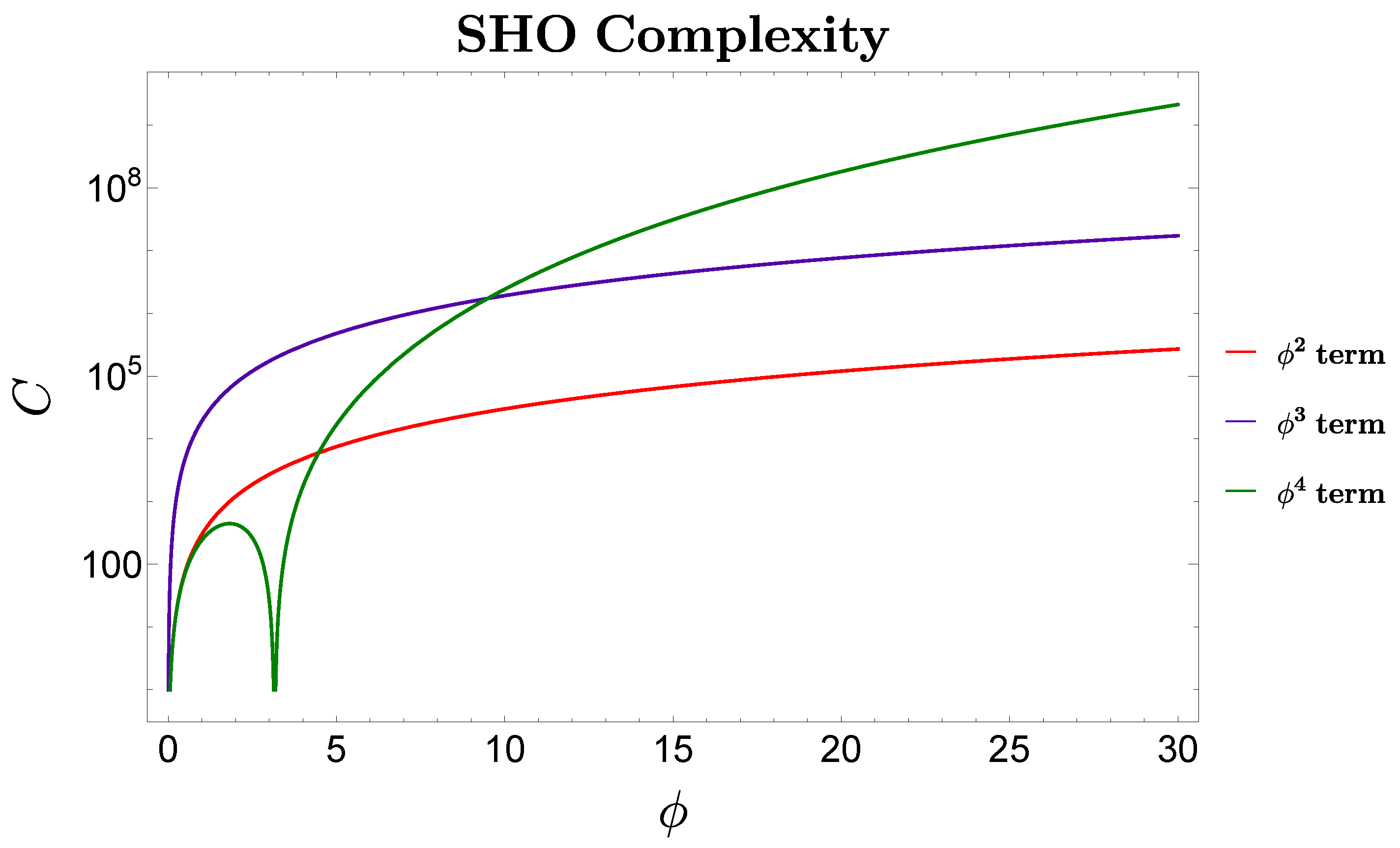
With the computed formulae for complexity for IHO and SHO in the previous sections, we plot the graphs using different values of parameters.

8.1. SHO

For SHO, the parameters involved are the mass m and coupling coefficient $\lambda$ for higher-order theories. We have chosen a simple linear coordinate transformation between the field variables x and $\theta$ and u, v. This ensures that the Hessian is a constant, and our computations become much more straightforward. The particular coefficients of the transformation have been chosen so that complexity is positive and rising for all cases.

In Figure 1 we have plotted the three different complexities for an intermediate value of mass, keeping the coupling coefficient fixed. We observe that the complexity rises and saturates as expected.

It is important to know how the complexity value behaves for different masses. For lighter particles, as we see in Figure 2, we see a slight overall decrease in the complexity values, but more importantly, we observe that the graph of ${\varphi }^3$ term tends very close to the ${\varphi }^2$ graph. We conclude that as the mass grows smaller, the ${\varphi }^3$ graph will inch closer and be indistinguishable from the ${\varphi }^2$ graph.

For larger masses, we see a stark difference. Here the graph of the ${\varphi }^4$ theory inches closer to the ${\varphi }^2$ graph as seen in Figure 3 and we can once again expect that it will become indistinguishable for much larger masses.

The other important parameter that we need to vary is the value of $\lambda$, and we start by seeing what will happen when it is made negative as seen in Figure 4. We know the behavior of the complexity remains the same, i.e., it grows and saturates as we go right. An exciting behavior occurs in the ${\varphi }^4$ graph. We see an initial rise and dip before the rise and saturation. This indicates that we have a zero in the ${\varphi }^4$ theory.

We observe no behavioral changes when we vary the specific value of $\lambda$ apart from the fact that for higher values, it saturates much quickly (pointing to a larger Lyapunov exponent) and saturates slower for smaller values (smaller Lyapunov exponent).

8.2. IHO

For the plots of IHO, we need to keep in mind that there are many more parametric values. We will do a graphical analysis mainly by varying mass and temperature. We will merely state the redundancy involved in other parameters and therefore explain our choice of fixing it.

• If one looks closer to the formulae given for IHO in Section 6 we see the value of the momentum-p just adds an overall factor that multiplies the function, thereby acting as a scaling factor. Hence we can set this to p = 1 without any issues.
• Another important parameter that might affect our plots is whether the value of $F-\gamma$ is Odd or Even. When it is even, we have positive complexity, and when it is odd, we find that we are dealing with negative complexity values, which we safely ignore in the present context of the discussion.

Before we proceed to vary the inverse temperature ($\beta$) and the mass (m), we can take a look at the general feature of the graphs of different perturbations in the field for both positive and negative $\lambda$ as we have done in Figure 5 and Figure 6.

We see that the complexity values in all perturbations rise for positive coupling coefficient but at different rates. In contrast, in the case of a negative coupling coefficient, we see that they decrease rapidly after an initial period of rising (almost an inverse behavior of the positive $\lambda$ case). We also observe symmetry for negative values of the field in the ${\varphi }^2+{\varphi }^4$ graph. It is important to note that although we can calculate the slope values, one cannot associate a Lyapunov exponent for the same because saturation does not exist. Maybe we can regard the slight rise and saturation before the dip in the case of negative Lambda values and associate a Lyapunov exponent to it.

In Figure 7, we have plotted how the complexity values vary when we vary the inverse temperature and the mass. Very similar behavior is observed in the case of ${\varphi }^2+{\varphi }^4$ perturbation, shown in Figure 8.

Since we have already established the behavior of the complexity in the case of negative $\lambda$, we take the liberty of not explicitly plotting the above variations in the inverse temperature and mass for that case. One has to imagine a decreasing (cannot associate a Lyapunov exponent) mirror inversion in the negatively valued domain of the field. This is true for the cases of both perturbations that we have discussed in the present context.

9. Quantum Chaos from Morse Function

The emergence of chaos in quantum phenomena can be estimated using an out-of-time-order correlation function that is firmly associated with the operator commutator, split up in time. However, the universal relation $\mathcal{C}=-ln\left(OTOC\right)$ relating complexity with OTOC [36,68,69,70,71,72,73,74] has been studied greatly in recent times to diagnose chaos in various physical models. This section will prove this universal relation for the supersymmetric case, relating the complexity with OTOC using the frame of Morse theory. We will comment on the upper bound of chaos, namely the Lyapunov exponent. In the above sections, by identifying the Morse function on a manifold with the cost function, we have calculated the complexity for supersymmetric field theories in various regimes in terms of the Hessian $H\left(f\right)$ and also have made use of the fact that the eigenvalues of supersymmetric Hamiltonian $H_t$ are concentrated near the critical points of the Morse function defined on the manifold. In this section, we will make use of the same facts and derive the universality relation.

Theorem 3.

Let $\varphi \left(t\right)$ be an integral curve which represents the state of the particle at various time, then if $x_1,\dots x_m$ be a local coordinate chart around a critical point $p\in M$ such that $\frac{\partial }{\partial x^1},\dots .,\frac{\partial }{\partial x^m}$ is an orthonormal basis for $T_{p}M$ with respect to the metric g, then for any $t\in R$ the out-of-time-correlator at p is equal to the exponential of the minus the matrix of the Hessian at p, i.e.,

$$\frac{\partial }{\partial x}{\varphi }_t{|}_p=exp(-H_p\left(f\right)t).$$

(92)

By identifying ${\varphi }_t$ as a smooth function on the surface of the manifold we have

$$\frac{d}{dt}\varphi (t,x)=-(\nabla f)\left(\frac{\partial }{\partial x}\varphi (t,x)\right).$$

(93)

By changing the order of differentiation for any $x\in M$ we obtain,

$$\frac{d}{dt}\left(\frac{\partial }{\partial x}\varphi (t,x)\right)=-\left(\frac{\partial }{\partial x}\nabla f\right)\left(\frac{\partial }{\partial x}\varphi (t,x)\right).$$

(94)

Therefore by defining:

$$\mathsf{\Phi }(t,x)=\frac{\partial }{\partial x}\varphi (t,x)$$

(95)

is a solution of the linear system of ODE’s:

$$\frac{d}{dt}\mathsf{\Phi }(t,x)=-\left(\frac{\partial }{\partial x}\nabla f\right)\mathsf{\Phi }(t,x).$$

(96)

Because $exp\left(-\left(\frac{\partial }{\partial x}\nabla f\right)t\right)$ is also a solution to the linear ODE’s, we finally obtain:

$$\mathsf{\Phi }(t,x)=\frac{\partial }{\partial x}\varphi (t,x)=exp\left(-\left(\frac{\partial }{\partial x}\nabla f\right)t\right).$$

(97)

Since the solution is unique, thereby, at the location of critical point p we have:

$$\frac{\partial }{\partial x}{\varphi }_t{|}_p=exp(-H_p\left(f\right)t)$$

(98)

Hence, by identifying the complexity of SUSY field theories with the Hessian as described in this paper, the above equation under good approximations could be written as:

$$\mathcal{C}=-ln\left(OTOC\right).$$

(99)

From the above equation, we could see that the Hessian of the Morse function, under good approximations, is perfectly consistent with universal relation and is of great interest to capture the effect of chaos in supersymmetric field theories.

We will now comment on the behavior of Lyapunov exponent in SUSY field theories, especially in the framework of an inverted harmonic oscillator under which it is expected to have chaotic features, depending upon the increase in the number of critical points as described in Section 6. Thus we could write the expression for complexity in the IHO regime as:

$${\mathcal{C}}_i\left(t\right)\approx cexp\left({\lambda }_{i}t\right)\forall i=1,2,\dots ,n.$$

(100)

It is to be noted that the above equation is valid only for the IHO. The index i indicates the higher-order quantum corrections in the Lagrangian for which the complexity has been measured, then mathematically Lyapunov exponent could be written as:

$${\lambda }_i=\left(\frac{dln{\mathcal{C}}_i\left(t\right)}{dt}\right)\forall i=1,2,\dots n.$$

(101)

Now, using the universal relation relating complexity with the Out-of-Time Ordered Correlation (OTOC) function, one could write:

$$OTOC=exp(-cexp\left(\lambda t\right))$$

(102)

where $\lambda$ is the Lyapunov exponent [75,76,77] which captures the effect of chaos in the quantum regime and relates different measures of complexity with OTOC through the universal relation. The above universal relation between complexities in different order of perturbations in the superpotential can be translated to the Lyapunov exponent through the MSS bound as:

$${\lambda }_i\le \lambda \le \frac{2\pi }{\beta }\forall i=1,2,\dots ,n.$$

(103)

where $\beta$ is the inverse temperature. We have shown that the Morse function could be used to classify the topology of surfaces and capture the effect of chaos in the quantum regime of supersymmetric field theories.

10. Conclusions

Out-of-order-correlation-function (OTOC) in the framework of supersymmetry has been studied before and, as a result, did not show any chaotic behavior in the regime of SHO. Our primary focus in this paper was to bring out the relationship between circuit complexity and Morse function and comment on the complexity of supersymmetric quantum field theory, in the regime of the simple and inverted harmonic oscillator (IHO), by formulating the potential of IHO as the generators of SL(2, Z) group. By pointing out the relationship between the cost and Morse function on a manifold, we have explicitly shown how the critical points on the surface encapsulate the action of the supersymmetric charge on the given reference state. We have explicitly made use of the fact that the eigenvalues of the supersymmetric Hamiltonian are concentrated near the critical points of the Morse function in the manifold, and then using the Witten index, which comments on the symmetry breaking of the theory, we commented on the complexity of the supersymmetric field theories for the IHO, which increases by a factor of exponential. For computations of complexity in the regime of the simple harmonic oscillator, we found out that circuit complexity did not show any dependence on initial conditions or exponential behavior. Next, we have the well known universal relation relating complexity and out-of-time ordered correlation function $\mathcal{C}=-ln\left(OTOC\right)$ using the general description of Morse theory.

• Remark I: The circuit complexity for supersymmetric field theories has very deep connections with the Morse function defined on the surface of the manifold. We have obtained the expression for complexity for SUSY field theories in terms of the Hessian of the Morse function. In doing so, we have made use of the fact the eigenvalues of the supersymmetric Hamiltonian are concentrated near the critical points of the Morse function.
• Remark II: The behaviour of complexity for supersymmetric field theories for the inverted harmonic oscillator is of prime importance, we have found that the growth of complexity in the regime of IHO is directly related to the growth of the number of critical points on the manifold, which in turn grows exponentially with respect to the superpotential, we observed similar behavior for higher-order quantum corrections namely ${\varphi }^3$ and ${\varphi }^4$ theories.
• Remark III: We have also computed complexity for the simple harmonic oscillator, and found out that circuit complexity did not show any dependence on initial conditions or exponential behavior. It is also worth mentioning that complexity for supersymmetric scalar field theories only depends on the absolute value of the non-dynamical auxiliary field. The F-term is identified with the gradient of the Morse function determines whether the supersymmetry is spontaneously broken or not depending upon whether the gradient has passed through the critical points. On passing through the critical points, we obtain F = 0 which means no zero energy supersymmetric ground states exist.
• Remark IV: We have proved the well known universal relation $\mathcal{C}=-ln\left(OTOC\right)$ which relates complexity with the out-of-time ordered correlation function for supersymmetric field theories using Morse theory. The out-of-time ordered correlation function is an excellent gadget to capture the effect of chaos in the quantum regime. In this paper, we have obtained an upper bound on the Lyapunov exponent and also commented on its various features for supersymmetric field theories purely for SHO and IHO in Table 1 and Table 2 using aspects of Morse Theory. The main point of Witten’s paper on supersymmetry and Morse theory was to provide supersymmetry with a mathematical structure. Like the Witten index, which tells if the supersymmetry is broken or not, various results would not have been possible by the normal description of particle physics.
• Remark V: We have found that complexity for supersymmetric field theories differ significantly from ordinary quantum field theories in the sense that for non-SUSY QFT complexity, slowly starts to increase at the critical point, however for SUSY field theories the graph rises fast initially and then gradually tends to saturate. The rate of saturation depends on the order of quantum corrections. The ${\varphi }^3$ theory saturates very rapidly and have the smallest Lyapunov exponent among the other studied perturbations, while the complexity for theory involving ${\varphi }^4$ term saturates slowly. For IHO, we observed that complexity increases exponentially and quickly rose to very high values unlike ordinary QFT where it has a linear growth.
• Remark VI: We have explicitly studied the dependence of mass on the behavior of circuit complexity and have observed that for massive fields there is a decrease in the rate of change of complexity for ${\varphi }^4$ theory, and it interesting to note that the graph becomes nearly indistinguishable from that of free field theory. However, for smaller masses, the complexity for ${\varphi }^3$ graph approaches to ${\varphi }^2$ slowly with a slight decrease in the rate of complexity. Hence, we expect an increase in the value of the Lyapunov exponent. In the case of IHO, we observe that as mass increases, the rate of change of complexity w.r.t $\varphi$ also increases.
• Remark VII: We have also commented on the behavior of complexity w.r.t the coupling constant $\lambda$ and have observed that for negatives values of $\lambda$ in the regime of SHO the saturation is slower for ${\varphi }^2$ and ${\varphi }^3$ perturbations and in the case of ${\varphi }^4$ theory their is a sudden dip at the initial stage to zero thereby right shifting the point of initial rise of complexity. In the case of IHO, the increase in the value of $\lambda$ results in an increase in the rate of change complexity; however, for negative values of $\lambda$ we found that complexity decreases exponentially SUSY field theories.

The future prospects of the present work are appended below:

• Prospect I: In this paper we have restricted ourselves to supersymmetric scalar field theories, however similar computations could be done for supersymmetric gauge and non-Abelian gauge theories by taking in consideration the dynamical D term [78,79], which would give further understanding about complexity and effect of chaos in supersymmetric field theories.
• Prospect II: circuit complexity for interacting quantum field theories and its relation with renormalization group has been studied by Arpan Bhattacharyya and collaborator and thus, it will be interesting to see what new mathematical structure does renormalization group flow brings out and how it is related to complexity [80,81,82].
• Prospect III: In this paper, we have computed the complexity for SUSY scalar field theories by making use of the properties of the Hessian matrix. However, we hope that this is not all [83]. The use of other remarkable properties of the Morse function could help in gaining a much broader perspective in supersymmetric field theories and its matter content and interactions and the effect it has on the expansion of universe [84].
• Prospect IV: The study of supersymmetry and its complexity in terms of Morse theory has given it a geometrical structure, however for theories of supergravity it is still not quit clear what the right mathematical structure is [85,86], we suppose that the work on this direction would bring interesting connections between quantum chaos and various other mathematical theories.

References

1. Lashkari, N.; McDermott, M.B.; Van Raamsdonk, M. Gravitational dynamics from entanglement ’thermodynamics’. J. High Energy Phys. 2014, 4, 195. [Google Scholar] [CrossRef] [Green Version]
2. Van Raamsdonk, M. Building up spacetime with quantum entanglement. Gen. Rel. Grav. 2010, 42, 2323–2329. [Google Scholar] [CrossRef]
3. Maldacena, J.; Susskind, L. Cool horizons for entangled black holes. Fortsch. Phys. 2013, 61, 781–811. [Google Scholar] [CrossRef] [Green Version]
4. Maldacena, J.M. The Large N limit of superconformal field theories and supergravity. Int. J. Theory Phys. 1999, 38, 1113–1133. [Google Scholar] [CrossRef] [Green Version]
5. Li, T.; Liu, J.; Xin, Y.; Zhou, Y. Supersymmetric SYK model and random matrix theory. J. High Energy Phys. 2017, 6, 111. [Google Scholar] [CrossRef]
6. Choudhury, S.; Dey, A.; Halder, I.; Janagal, L.; Minwalla, S.; Poojary, R. Notes on melonic O(N)q−1 tensor models. J. High Energy Phys. 2018, 6, 94. [Google Scholar] [CrossRef] [Green Version]
7. Nakata, Y.; Takayanagi, T.; Taki, Y.; Tamaoka, K.; Wei, Z. New holographic generalization of entanglement entropy. Phys. Rev. D 2021, 103, 026005. [Google Scholar] [CrossRef]
8. Barbón, J.; Martin-Garcia, J.; Sasieta, M. A generalized Momentum/Complexity correspondence. J. High Energy Phys. 2021, 2021, 250. [Google Scholar] [CrossRef]
9. Yang, R.Q.; An, Y.S.; Niu, C.; Zhang, C.Y.; Kim, K.Y. What kind of “complexity” is dual to holographic complexity? Eur. Phys. J. C 2022, 82, 262. [Google Scholar] [CrossRef]
10. Susskind, L. Entanglement and Chaos in de Sitter Holography: An SYK Example. JHAP 2021, 1, 1. [Google Scholar]
11. Emparan, R.; Frassino, A.M.; Sasieta, M.; Tomašević, M. Holographic complexity of quantum black holes. J. High Energy Phys. 2022, 2022, 204. [Google Scholar] [CrossRef]
12. Bhattacharya, A.; Bhattacharyya, A.; Nandy, P.; Patra, A.K. Islands and complexity of eternal black hole and radiation subsystems for a doubly holographic model. J. High Energy Phys. 2021, 2021, 135. [Google Scholar] [CrossRef]
13. Jiang, J.; Zhang, M. Holographic complexity of the electromagnetic black hole. Eur. Phys. J. C 2020, 80, 85. [Google Scholar] [CrossRef]
14. Auzzi, R.; Baiguera, S.; Legramandi, A.; Nardelli, G.; Roy, P.; Zenoni, N. On subregion action complexity in AdS3 and in the BTZ black hole. J. High Energy Phys. 2020, 2020, 66. [Google Scholar] [CrossRef] [Green Version]
15. An, Y.S.; Cai, R.G.; Peng, Y. Time dependence of holographic complexity in Gauss-Bonnet gravity. Phys. Rev. D 2018, 98, 106013. [Google Scholar] [CrossRef] [Green Version]
16. Susskind, L. Entanglement is not enough. Fortsch. Phys. 2016, 64, 49–71. [Google Scholar] [CrossRef] [Green Version]
17. Susskind, L.; Zhao, Y. Switchbacks and the Bridge to Nowhere. arXiv 2014, arXiv:1408.2823. [Google Scholar]
18. Shenker, S.H.; Stanford, D. Black holes and the butterfly effect. J. High Energy Phys. 2014, 3, 67. [Google Scholar] [CrossRef] [Green Version]
19. Swingle, B.; Van Raamsdonk, M. Universality of Gravity from Entanglement. arXiv 2014, arXiv:1405.2933. [Google Scholar]
20. Choudhury, S.; Panda, S. Entangled de Sitter from stringy axionic Bell pair I: An analysis using Bunch-Davies vacuum. Eur. Phys. J. 2018, C78, 52. [Google Scholar] [CrossRef] [Green Version]
21. Choudhury, S.; Panda, S. Quantum entanglement in de Sitter space from stringy axion: An analysis using α vacua. Nucl. Phys. 2019, B943, 114606. [Google Scholar] [CrossRef]
22. Choudhury, S.; Panda, S.; Singh, R. Bell violation in the Sky. Eur. Phys. J. 2017, C77, 60. [Google Scholar] [CrossRef]
23. Belin, A.; Myers, R.C.; Ruan, S.M.; Sárosi, G.; Speranza, A.J. Does Complexity Equal Anything? Phys. Rev. Lett. 2022, 128, 81602. [Google Scholar] [CrossRef]
24. Roberts, D.A.; Stanford, D.; Susskind, L. Localized shocks. J. High Energy Phys. 2015, 3, 51. [Google Scholar] [CrossRef] [Green Version]
25. Brown, A.R.; Roberts, D.A.; Susskind, L.; Swingle, B.; Zhao, Y. Complexity, action, and black holes. Phys. Rev. D 2016, 93, 86006. [Google Scholar] [CrossRef] [Green Version]
26. Brown, A.R.; Roberts, D.A.; Susskind, L.; Swingle, B.; Zhao, Y. Holographic Complexity Equals Bulk Action? Phys. Rev. Lett. 2016, 116, 191301. [Google Scholar] [CrossRef]
27. Brown, A.R.; Susskind, L. Second law of quantum complexity. Phys. Rev. D 2018, 97, 86015. [Google Scholar] [CrossRef] [Green Version]
28. Chagnet, N.; Chapman, S.; de Boer, J.; Zukowski, C. Complexity for conformal field theories in general dimensions. Phys. Rev. Lett. 2022, 128, 51601. [Google Scholar] [CrossRef]
29. Bhattacharyya, A. Circuit complexity and (some of) its applications. Int. J. Modern Phys. E 2021, 30, 2130005. [Google Scholar] [CrossRef]
30. Guo, M.; Hernandez, J.; Myers, R.C.; Ruan, S.M. Circuit complexity for coherent states. J. High Energy Phys. 2018, 2018, 11. [Google Scholar] [CrossRef] [Green Version]
31. Chapman, S.; Heller, M.P.; Marrochio, H.; Pastawski, F. Toward a definition of complexity for quantum field theory states. Phys. Rev. Lett. 2018, 120, 121602. [Google Scholar] [CrossRef] [PubMed] [Green Version]
32. Akhtar, S.; Choudhury, S.; Chowdhury, S.; Goswami, D.; Panda, S.; Swain, A. Open Quantum Entanglement: A study of two atomic system in static patch of de Sitter space. Eur. Phys. J. 2020, C80, 748. [Google Scholar] [CrossRef]
33. Banerjee, S.; Choudhury, S.; Chowdhury, S.; Knaute, J.; Panda, S.; Shirish, K. Thermalization in Quenched de Sitter Space. arXiv 2021, arXiv:2104.10692. [Google Scholar]
34. Krishnan, C.; Mohan, V. Hints of gravitational ergodicity: Berry’s ensemble and the universality of the semi-classical Page curve. J. High Energy Phys. 2021, 5, 126. [Google Scholar] [CrossRef]
35. Bhagat, K.Y.; Bose, B.; Choudhury, S.; Chowdhury, S.; Das, R.N.; Dastider, S.G.; Gupta, N.; Maji, A.; Pasquino, G.D.; Paul, S. The Generalized OTOC from Supersymmetric Quantum Mechanics: Study of Random Fluctuations from Eigenstate Representation of Correlation Functions. Symmetry 2020, 13, 44. [Google Scholar] [CrossRef]
36. Choudhury, S. The Cosmological OTOC: A New Proposal for Quantifying Auto-correlated Random Non-chaotic Primordial Fluctuations. arXiv 2021, arXiv:202102.0616. [Google Scholar]
37. Dowling, M.R.; Nielsen, M.A. The geometry of quantum computation. arXiv 2006, arXiv:quant-ph/0701004. [Google Scholar]
38. Jefferson, R.; Myers, R.C. Circuit complexity in quantum field theory. J. High Energy Phys. 2017, 10, 107. [Google Scholar] [CrossRef] [Green Version]
39. Nielsen, M.A. A geometric approach to quantum circuit lower bounds. arXiv 2005, arXiv:quant-ph/0502070. [Google Scholar]
40. Auzzi, R.; Baiguera, S.; De Luca, G.B.; Legramandi, A.; Nardelli, G.; Zenoni, N. Geometry of quantum complexity. arXiv 2021, arXiv:2011.07601. [Google Scholar]
41. Roberts, D.A.; Yoshida, B. Chaos and complexity by design. J. High Energy Phys. 2017, 4, 121. [Google Scholar] [CrossRef] [Green Version]
42. Choudhury, S.; Dutta, A.; Ray, D. Chaos and Complexity from Quantum Neural Network: A study with Diffusion Metric in Machine Learning. J. High Energy Phys. 2021, 4, 138. [Google Scholar] [CrossRef]
43. Yang, R.Q. Complexity for quantum field theory states and applications to thermofield double states. Phys. Rev. D 2018, 97, 66004. [Google Scholar] [CrossRef] [Green Version]
44. Brown, A.R.; Susskind, L.; Zhao, Y. Quantum Complexity and Negative Curvature. Phys. Rev. D 2017, 95, 45010. [Google Scholar] [CrossRef] [Green Version]
45. Khan, R.; Krishnan, C.; Sharma, S. Circuit Complexity in Fermionic Field Theory. Phys. Rev. D 2018, 98, 126001. [Google Scholar] [CrossRef] [Green Version]
46. Adhikari, K.; Choudhury, S.; Chowdhury, S.; Shirish, K.; Swain, A. Circuit complexity as a novel probe of quantum entanglement: A study with black hole gas in arbitrary dimensions. Phys. Rev. D 2021, 104, 65002. [Google Scholar] [CrossRef]
47. Bhattacharyya, A.; Chemissany, W.; Haque, S.S.; Murugan, J.; Yan, B. The Multi-faceted Inverted Harmonic Oscillator: Chaos and Complexity. SciPost Phys. Core 2021, 4, 002. [Google Scholar] [CrossRef]
48. Subramanyan, V.; Hegde, S.S.; Vishveshwara, S.; Bradlyn, B. Physics of the Inverted Harmonic Oscillator: From the lowest Landau level to event horizons. Ann. Phys. 2021, 435, 168470. [Google Scholar] [CrossRef]
49. Barton, G. Quantum Mechanics of the Inverted Oscillator Potential. Ann. Phys. 1986, 166, 322. [Google Scholar] [CrossRef]
50. Hawking, S. Black hole explosions. Nature 1974, 248, 30–31. [Google Scholar] [CrossRef]
51. Birrell, N.; Davies, P. Quantum Fields in Curved Space. Cambridge Monographs on Mathematical Physics; Cambridge University Press: Cambridge, UK, 1984. [Google Scholar]
52. Crispino, L.C.; Higuchi, A.; Matsas, G.E. The Unruh effect and its applications. Rev. Mod. Phys. 2008, 80, 787–838. [Google Scholar] [CrossRef] [Green Version]
53. Read, N.; Rezayi, E. Hall viscosity, orbital spin, and geometry: Paired superfluids and quantum Hall systems. Phys. Rev. B 2011, 84, 85316. [Google Scholar] [CrossRef] [Green Version]
54. Fecko, M. Differential Geometry and Lie Groups for Physicists; Cambridge University Press: Cambridge, UK, 2011. [Google Scholar]
55. Kerr, M. Notes on the representation theory of SL2 (R). Hodge Theory Complex Geom. Represent. Theory 2014, 608, 173. [Google Scholar]
56. Bott, R. Lectures on Morse theory, old and new. Bull. N. Ser. Am. Math. Soc. 1982, 7, 331–358. [Google Scholar] [CrossRef] [Green Version]
57. Austin, D.M.; Braam, P.J. Morse-Bott theory and equivariant cohomology. In The Floer Memorial Volume; Springer: Berlin/Heidelberg, Germany, 1995; pp. 123–183. [Google Scholar]
58. Milnor, J. Morse Theory (AM-51); Princeton University Press: Princeton, NJ, USA, 2016; Volume 51. [Google Scholar]
59. Witten, E. Constraints on Supersymmetry Breaking. Nucl. Phys. B 1982, 202, 253. [Google Scholar] [CrossRef]
60. Witten, E. Supersymmetry and Morse theory. J. Diff. Geom. 1982, 17, 661–692. [Google Scholar] [CrossRef]
61. Drees, M. An Introduction to supersymmetry. In Proceedings of the Inauguration Conference of the Asia Pacific Center for Theoretical Physics (APCTP), Seoul, Korea, 1–6 February 1996. [Google Scholar]
62. Witten, E. Dynamical Breaking of Supersymmetry. Nucl. Phys. B 1981, 188, 513. [Google Scholar] [CrossRef]
63. Weinberg, S. The Quantum Theory of Fields. Volume 3: Supersymmetry; Cambridge University Press: Cambridge, UK, 2013. [Google Scholar]
64. Gates, S.J.; Grisaru, M.T.; Rocek, M.; Siegel, W. Superspace or One Thousand and One Lessons in Supersymmetry. In Frontiers in Physics; Springer: Berlin/Heidelberg, Germany, 1983; Volume 58. [Google Scholar]
65. Quevedo, F.; Krippendorf, S.; Schlotterer, O. Cambridge Lectures on Supersymmetry and Extra Dimensions; Springer: Berlin/Heidelberg, Germany, 2010. [Google Scholar]
66. Shirman, Y. Introduction to Supersymmetry and Supersymmetry Breaking. In Proceedings of the Theoretical Advanced Study Institute in Elementary Particle Physics: The Dawn of the LHC Era; Springer: Berlin/Heidelberg, Germany, 2010; pp. 359–422. [Google Scholar]
67. Wess, J.; Zumino, B. Supergauge Invariant Extension of Quantum Electrodynamics. Nucl. Phys. B 1974, 78, 1. [Google Scholar] [CrossRef] [Green Version]
68. Choudhury, S.; Chowdhury, S.; Gupta, N.; Mishara, A.; Selvam, S.P.; Panda, S.; Pasquino, G.D.; Singha, C.; Swain, A. Circuit Complexity from Cosmological Islands. Symmetry 2021, 13, 1301. [Google Scholar] [CrossRef]
69. Bhargava, P.; Choudhury, S.; Chowdhury, S.; Mishara, A.; Selvam, S.P.; Panda, S.; Pasquino, G.D. Quantum Aspects of Chaos and Complexity from Bouncing Cosmology: A Study with Two-Mode Single Field Squeezed State Formalism. SciPost Phys. Core 2021, 4, 026. [Google Scholar] [CrossRef]
70. Hashimoto, K.; Murata, K.; Yoshii, R. Out-of-time-order correlators in quantum mechanics. J. High Energy Phys. 2017, 10, 138. [Google Scholar] [CrossRef] [Green Version]
71. Choudhury, S. The Cosmological OTOC: Formulating new cosmological micro-canonical correlation functions for random chaotic fluctuations in Out-of-Equilibrium Quantum Statistical Field Theory. Symmetry 2020, 12, 1527. [Google Scholar] [CrossRef]
72. Choudhury, S.; Panda, S. Cosmological Spectrum of Two-Point Correlation Function from Vacuum Fluctuation of Stringy Axion Field in De Sitter Space: A Study of the Role of Quantum Entanglement. Universe 2020, 6, 79. [Google Scholar] [CrossRef]
73. Choudhury, S.; Mukherjee, A.; Chauhan, P.; Bhattacherjee, S. Quantum Out-of-Equilibrium Cosmology. Eur. Phys. J. 2019, C79, 320. [Google Scholar] [CrossRef]
74. BenTov, Y. Schwinger-Keldysh Path Integral for the Quantum Harmonic Oscillator. arXiv 2021, arXiv:2102.05029. [Google Scholar]
75. Maldacena, J.; Shenker, S.H.; Stanford, D. A bound on chaos. J. High Energy Phys. 2016, 8, 106. [Google Scholar] [CrossRef] [Green Version]
76. Bunakov, V. Quantum signatures of chaos or quantum chaos? Phys. Atom. Nucl. 2016, 79, 995–1009. [Google Scholar] [CrossRef]
77. Han, X.; Hartnoll, S.A. Quantum Scrambling and State Dependence of the Butterfly Velocity. Sci. Post Phys. 2019, 7, 45. [Google Scholar] [CrossRef]
78. Itoyama, H.; Maru, N. D-term Triggered Dynamical Supersymmetry Breaking. Phys. Rev. D 2013, 88, 25012. [Google Scholar] [CrossRef] [Green Version]
79. Piguet, O. Introduction to supersymmetric gauge theories. In Proceedings of the 1st School on Field Theory and Gravitation; IEEE: Hoboken, NJ, USA, 2012. [Google Scholar]
80. Bonini, M.; Vian, F. Wilson renormalization group for supersymmetric gauge theories and gauge anomalies. Nucl. Phys. B 1998, 532, 473–497. [Google Scholar] [CrossRef] [Green Version]
81. Kazakov, D. Supersymmetry in particle physics: The renormalization group viewpoint. Phys. Rep. 2001, 344, 309–353. [Google Scholar] [CrossRef] [Green Version]
82. Maruyoshi, K.; Song, J. Enhancement of Supersymmetry via Renormalization Group Flow and the Superconformal Index. Phys. Rev. Lett. 2017, 118, 151602. [Google Scholar] [CrossRef] [PubMed] [Green Version]
83. Murugan, J.; Stanford, D.; Witten, E. More on Supersymmetric and 2d Analogs of the SYK Model. J. High Energy Phys. 2017, 8, 146. [Google Scholar] [CrossRef]
84. Bilic, N. Supersymmetric dark energy. Rom. J. Phys. 2012, 57, 793–802. [Google Scholar]
85. Coimbra, A.; Strickland-Constable, C.; Waldram, D. Supergravity as Generalised Geometry I: Type II Theories. J. High Energy Phys. 2011, 11, 91. [Google Scholar] [CrossRef] [Green Version]
86. Lazaroiu, C.; Shahbazi, C. Four-Dimensional Geometric Supergravity and Electromagnetic Duality: A Brief Guide For Mathematicians. arXiv 2020, arXiv:2006.16157. [Google Scholar]
Figure 1. Complexity against ϕ for m = 1 , λ = 1 .
Symmetry 14 01656 g001
Figure 2. Complexity against ϕ for m = 0.01 , λ = 1 .
Symmetry 14 01656 g002
Figure 3. Complexity against ϕ for m = 100 , λ = 1 .
Symmetry 14 01656 g003
Figure 4. Complexity against ϕ for m = 1 , λ = 1 .
Symmetry 14 01656 g004
Figure 5. Complexity against ϕ for different perturbations of field with λ = 1 .
Symmetry 14 01656 g005
Figure 6. Complexity against ϕ for different perturbations of field with λ = 1 .
Symmetry 14 01656 g006
Figure 7. Behavior of the complexity of ϕ 2 + ϕ 4 perturbation with varying β and m. (a) Variation of inverse temperature; (b) Variation of mass.
Symmetry 14 01656 g007
Figure 8. Behavior of the complexity of ϕ 2 + ϕ 3 perturbation with varying β and m. (a) Variation of inverse temperature; (b) Variation of mass.
Symmetry 14 01656 g008