Abstract
Building on a modified version of the Haantjes path-based curvature, this article offers a novel measure that considers the direction of a stream of associations in a semantic network and estimates the extent to which any single association attracts the upcoming associations to its environment—in other words, to what degree one explores that environment. We demonstrate that our measure differs from Haantjes curvature and confirm that it expresses the extent to which a stream of associations remains close to its starting point. Finally, we examine the relationship between our measure and accessibility to knowledge stored in memory. We demonstrate that a high degree of attraction facilitates the retrieval of upcoming words in the stream. By applying methods from differential geometry to semantic networks, this study contributes to our understanding of strategic search in memory.
1. Introduction
Humans desire information and spend an extensive amount of time searching for it. Many studies have focused on search strategies in the external world [1,2,3,4]. But the search for information occurs internally, too, through the exploration of information stored in memory. The significance of this internal search becomes clear when knowledge is defined as the link between units of information. Under this definition, a person can acquire new knowledge by making new connections or strengthening existing ones between units of information that are already stored in memory.
One way to explore search strategies in the internal world is to investigate transitions between words in a stream of associations produced by a semantic retrieval task. In a widely used task, participants produce, over the course of one minute, as many words as possible within a semantic category such as animals. Such a task enables us to explore the different search patterns that people use to retrieve information from memory.
Previous studies have found that words retrieved from memory tend to be bound into semantic clusters, and that once a specific cluster of words is exhausted, the agent moves on to another cluster [5]. Based on this phenomenon, Hills et al. [6] suggested that word retrieval is based on a local strategy, namely the word’s similarity to the previous word in a semantic space. If the agent finds no similar words, she switches to a new word, relying for this new retrieval on a global strategy based on the word’s frequency. An alternative account, suggested by Abbott et al. [7], views semantic content as a network and search as simply a random walk on that network.
These studies offer comprehensive word-retrieval strategies, whether switching from one cluster to another or walking randomly on the network, to describe how people search for information in memory. Our approach is different: we focus on the way strategy changes as a function of the attention that an agent gives to the present word. Our basic intuition is that the greater a word’s attraction—in other words, the more effectively a word captures an agent’s attention—the more fully an agent explores the semantic vicinity of that word, with the result being an increase in the number of related words that are retrieved. It is worth pointing out here that we use “attraction” when we describe the behavior of a word in its semantic environment and “attention” when we examine that behavior through the lens of an agent’s degree of attention to the word.
The novel measure we introduce in this study estimates the level of attraction of word S—in other words, to what extent S attracts the subsequent words so that the stream of associations remains in S’s semantic environment. An analogy may help to clarify this notion. Imagine two individuals leaving the house at the same time, the first one with the goal of removing weeds around the house and the second one with the goal of shopping. Although they each end up walking a total of 50 m, the first person does all that walking within a small radius of the house, while the second person walks within a much larger radius. The length of the two people’s paths is equal, but the first person stays closer to the starting point than the second person. The path of this first person is analogous to the stream of associations that stays in the semantic vicinity of a highly attractive word.
At this point it is important for us to clarify the assumptions that underlie our approach to the word-based internal search. Based on Nachshon et al. [8], we distinguish between semantic and attended spaces. Semantic space consists of all the concepts that an agent has come to know. Attended space, which is a subset of semantic space, comprises only the group of words to which the agent pays attention at time t. This group includes the specific word that is singled out by the stream of associations at time t—what we term the word of maximal attention—as well as a larger set of words. In this conception, the word about which the agent continues to seek information remains within the set of words to which the agent is paying attention. In the terminology we have introduced, the word of maximal attention remains within the attended space. Let us say that in time t the word of maximal attention is “water” and in time t + 1 the word of maximal attention is “tree”. If the agent sustains attention to “water”, then “water” remains in the set of words to which the agent is attentive in time t + 1, and so her next association might be “sea”. As it is new to the literature, we want to emphasize the claim that upcoming words remain related to S’s semantic context. Especially noteworthy is our claim that the upcoming words remain related to S’s semantic context.
We offer two explanations for why the word S remains in the attended space. The first possibility, which we call the attention-oriented search, is that the agent sustains attention to S, and therefore S remains in the attended space. The second possibility, which we call the greedy search, is that S is close to many other words. The difference between these explanations lies in the role of the word S. The attention-oriented search assumes that S influences the way one continues to retrieve words. By contrast, the greedy search assumes that words of maximal attention are surrounded by many interconnected words. Since the agent has a high probability of passing from one of those words to another, the agent can continue to retrieve words in the vicinity of the word of maximal attention, even without sustaining attention to that specific word.
The difference between these two types of searches is an important factor in our novel measure, which takes into account the length of the path . A simple explanation for the extent to which a path stays in the vicinity of word is the greedy search, in which the path flows from one word to the next closest word. Thus, the shorter the path is, the more it stays in the vicinity of . But this explanation is insufficient, because one can produce a short path from to that moves away in a “straight line” from the starting point. In other words, the shortness of a path does not necessarily mean that the path remains in the vicinity of the initial word . To deal with this problem, we take into account an additional quantity that estimates the “radius” of the path from and expresses the extent to which the path has moved away from that “radius”. A greedy approach would claim that the smaller the “radius” is, the more the path remains in the vicinity of the starting word. But this claim leads to non-intuitive results, since it would not differentiate between short and long paths for a constant “radius”.
By combining both quantities, our measure can account for a long path in a small “radius”, meaning a long path that stays in the vicinity of the starting word. When the “radius” quantity stays constant, the contribution of path length is the reverse of what occurs in the greedy approach: given a constant “radius”, the longer the path is, the more it stays in the vicinity of the starting word. The combination of quantities also allows us to draw a distinction between short and long paths with a constant “radius”. Our empirical analysis will differentiate between a greedy search and an attention-oriented search.
The theoretical foundations of our attraction measure rely on the notion of Ricci curvature. The classic formulation is defined on smooth manifolds and measures the deviation of the manifold from being locally Euclidean in various tangential directions. Since Ricci curvature is associated with a vector (direction) in smooth manifolds, it is an edge-measure in the discrete case. Several studies over the last decades have investigated the notion of curvature for discrete spaces [9,10,11,12] and demonstrated its practical applications in areas such as image processing [13], finance [14,15], biological networks [16,17,18] and various real-world networks [19]. This study’s conceptual contribution concerns the extent to which a vertex attracts a set of vertices to its vicinity; methodologically, the contribution is the implementation of a modified version of Haantjes curvature into a real-world network. To engage in this analysis, this study proposes a novel interpretation of a path curvature whose theoretical foundations were laid by Haantjes (1947) and detailed by Saucan (2015). This modified version of Haantjes curvature determines how an actual path is related to its starting point.
This paper belongs to a larger study that is described in Nachson et al. [20] and that lays the groundwork for relationships between network features and cognitive properties. That study introduced a novel interpretation for the notion of curvature in a semantic hyper-graph and suggested that Ricci-curvature explains “movement” on the graph by predicting the probability of the upcoming word. That research, however, did not address the influence of a concept’s attraction on movement downstream, and it is this issue that we seek to address here.
Our study is innovative in two important ways. First, while previous literature investigated mainly an edge-based curvature that takes into account only triangles—in other words, simple paths of length 2—we consider any path length. Moving from an edge-based to a path-based approach allows us to estimate the attributes of sets of vertices rather than pairs of vertices, and this means that our investigation includes the relationship between path curvature and accessibility to the set of words that belongs to the path. Second, we focus on actual paths, which are the actual lists of words that participants have produced, while previous literature has focused on possible paths, which are the paths that can be drawn on the graph by connecting vertices for which the distance is defined.
To validate our measure psychologically, we examine the relationship between a word-based strategy search, which is measured by a word’s level of attraction, and accessibility, which is measured by velocity, or the duration of time it takes to retrieve a word. We hypothesize that the more a word attracts other words to its vicinity, the faster the agent will retrieve the set of attracted words. This claim rests on a definition of the attractive word as a word that attracts a set of words to its vicinity. To remain in the vicinity of S means that one “sees” the words in S’s vicinity more in the light of S than in the light of other words. Another way of saying this is that the upcoming words stay within the semantic context that S produces and that we expect the set of words that belong to this context to be retrieved more quickly. This claim is consistent with the finding that semantic context facilitates the retrieval of words from memory [21]. We detect a significant and non-trivial negative relationship such that the higher the level of a word’s attraction, the higher its level of velocity (i.e., the shorter the transition time within its set of consecutive words) even when we control for greedy search and word location. Finally, we find that the attention-oriented search predicts velocity better than the greedy search.
The rest of this paper is organized as follows. Section 1 presents the semantic case study data we used in this research, along with some basic assumptions. Section 2 focuses on the theoretical perspective and offers our novel measure, based on Haantjes–Ricci curvature, to quantify each word’s level of attraction in a word-based strategic search. Section 3 consists of three parts. First, we propose an initial validation of our assumption that an attractive path is one that remains close to the starting word; second, we examine the relationship between attraction and Haantjes–Ricci-curvature, and third, we show that the attraction of a word based on the way people actually retrieve words is not explained by a greedy search. Section 4 focuses on the semantic case study and proposes a psychological validation by examining the relationship between a word-based strategy search, which we measure by level of attraction, and accessibility to information stored in memory, which we measure by velocity. Finally, we present our conclusions in Section 5.
2. Data and Network Construction
By presenting ways to measure psychological phenomena, this study offers potential approaches to real-world problems. Let us first present the data of our case study.
The experiment was conducted on two groups (Ntotal = 2047), both consisting of native Hebrew speakers. One group was recruited from the Hebrew University of Jerusalem (HUJI: N = 691; M:F = 1:1.002; mean age = 24.6 years; range: 18–39); the members of this group received coupons for coffee. The second group (P4A: N = 1356; M:F = 1:1.96; mean age = 29.07 years; range: 18–40) was recruited through the website www.panel4all.co.il (accessed on 23 November 2019), and participants were compensated with gift certificates from the panel4all organization. The ethics committee of the Department of Psychology at the Hebrew University of Jerusalem approved all experimental procedures.
Participants were given one minute in a category fluency test (CFT); the task was to produce as many unique words as possible within the semantic category of animal names. Participants from HUJI were recorded on a Philips DVT4010, and soundtracks were transcribed with the PRAAT program [22], which gave us the words as well as the time signatures for the beginning and end of each word. Participants from P4A were recorded on a phone application, and these soundtracks, too, were transcribed via PRAAT.
Two lists were generated for each participant: a list of words and a list of timestamps, with each timestamp indicating the start time of the word’s retrieval. The timestamps start at 0, indicating the beginning of the recording, and end at 60.
All of the Python code and raw data are publicly available via OSF (https://osf.io/w36tc/ accessed on 6 June 2020).
At this point it is important to emphasize that, as suggested by Nachshon et al. [20], we are dealing with actual paths, not possible paths; as far as we know, our grounding in actual paths is unique in the literature. While possible paths can be drawn on the network by connecting vertices for which the distance is defined, actual paths consist of the list of words provided by a participant. In our study, actual paths form the basis for constructing the semantic graph and examining the level of attraction and velocity. Since, as we will explain, velocity is derived from actual timestamps and attraction is derived from distances based on actual timestamps, the two measures are grounded in the same data. In the third part of our Results section, we will demonstrate that the connection between velocity and attraction is non-trivial in the case of actual paths. The situation is different in shuffled paths, which are produced by shuffling the order of all lists of words produced.
We begin by describing the manner in which we construct the semantic graph. Let be an edge-weighted and directed graph, with a set of vertices and a set of edges or links between words and in V. The words are the vertices, and the edges reflect the relationship between words. The R-neighbors of vertex v are the group of vertices at a distance from . The weight is based on the assumption that the closer the semantic relationship between two words, the faster the subject moves from one of those words to the other [23]. The weights of the edges are based on Nachshon’s proposal [24] and are calculated by a “distance” function that assumes, as expected for a metric, that the “distance” is non-negative. However, we do not assume symmetry such that . We also allow violation of the triangle inequality. Thus, our “distances” do not constitute a true metric.
Our “distance” function calculates the weights of the edges as follows. For any ordered pair of vertices , p = p(s) is a sublist of participant s; the sublist starts at and ends at and denotes the amount of normalized time that it took s to move from to . Here, each timestamp was normalized by the number of words that s produced. The “distance” function has two free variables that determine the upper and lower boundaries, WS (window size) and MS (minimum subjects):
- The upper boundary window size (WS), which is an integer, defines the maximum number of words between . The sublist p is therefore taken into account when the number of words between and is less than or equal to the number WS.
- MS is an integer defining the lower boundary, which is the minimum number of p’s containing and in that order, and with at most WS words between them.
Let P be the set of the number of times it took any p to traverse from to up to WS words. Then, the weight between the ordered pair and is defined as being the median of the numbers in the set P, if |P| > MS. Otherwise, no distance between and will be defined. In other words, a distance is well-defined if |P| > MS. A path’s length is the sum of the weights (or distances) of the edges that compose the path.
Note that not every pair of vertices i, j gets a weight, only those pairs that at least MS subject retrieved i and then j when the number of words in-between them is at most WS.
3. Theory
In this section, we present our novel measure, a modified version of Haantjes curvature [11,12,14]. Our measure estimates to what extent an actual path that started at word S remains in the vicinity of S. We compare two quantities. The first represents the length of the path and is simply the sum of distances between words in the path. The second represents the “radius” of the path by taking the word that is farthest from the starting point. The greater the path length and the smaller the “radius”, the more the path remains in the vicinity of the starting word.
This measure is path-based; more precisely, it estimates the level of attraction of a word in a path. Nonetheless, it can be generalized to estimate a vertex’s attraction level as well. We claim that ’s level of attraction can be measured by the median of the lengths of the paths in which appears as the first vertex. The greater the median is, the greater is ’s level of attraction.
3.1. Haantjes-Ricci Curvature
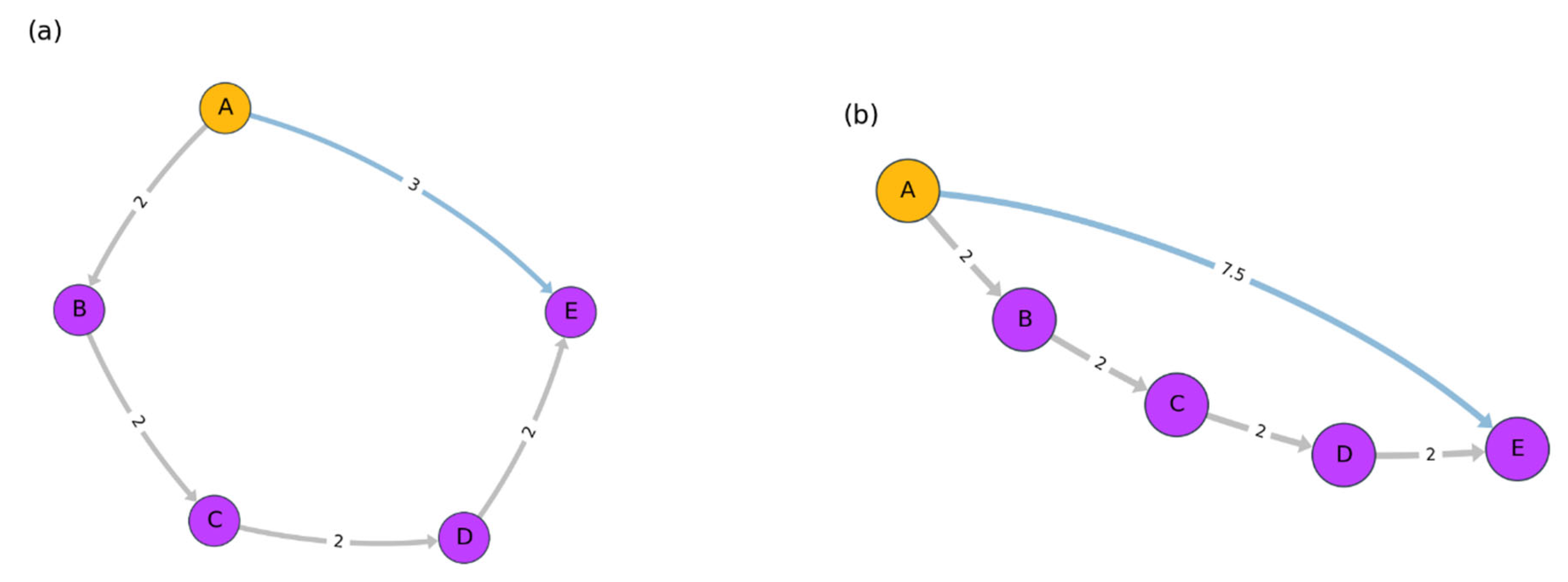
We base our measure on Haantjes–Ricci curvature (Figure 1), which is derived from a purely metric notion [11].
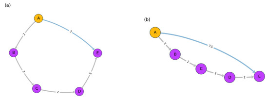
Figure 1.
Toy example for Haantjes curvature. In both figures, and , represented by gray edges. Regarding the second quantity the value is represented by a blue edge. The value of the path in (a) is and for (b) is . Hence, the path length in (a) is more curved and circulates in a smaller “radius” compared to the path length in (b).
Definition 1.
Let (M, d) be a metric space, let Cbe a simple curve, and let a,b,c∈C, a ≠ c ≠b, where b is between a and c. The Haantjes curvature of C at the point b is defined as follows [12]:
wheredenotes the length of the arc ab ∪ bc ⊂ c, anddenotes the length of the chord, meaning the distance fromto.
Note that, when , is equal to zero. As we are not necessarily considering a proper metric in this paper, when the chord is longer than the path length, the right-hand side of (1) will be negative. In this case we assign a “-” sign to .
Remark 1.
The cube term in the denominator of (1) is considered for scaling reasons; in the simplified Equation (2), the scaling will be removed (see, for example, [25]).
It is natural to adapt the notion of Haantjes curvature to graphs by replacing the arc ab ∪ bc with a path of length . More precisely we have
Definition 2.
Letbe a directed path between the verticesandin a networkThe simplified Haantjes curvature of the pathis defined as follows [14]:
Given that vertex-based notions, while less expressive, are more common in the literature, it is natural to derive a natural notion of Haantjes curvature of a vertex.
Definition 3.
The Haantjes–scalar curvature ofin a graphis defined as follows:
wheredenotes the simple paths that are starting at vertex.
3.2. Simplified and Modified Haantjes Curvature
In our simplified and modified version of Haantjes curvature, we compare two quantities. The first represents the length of an actual path, and the second estimates the maximal distance back to the starting point. For the graph G and the path , with the weights , let denote the set of edges when is the first vertex in the path . More precisely, we have the following:
Definition 4.
The simplified and modified Haantjes curvature is defined as follows:
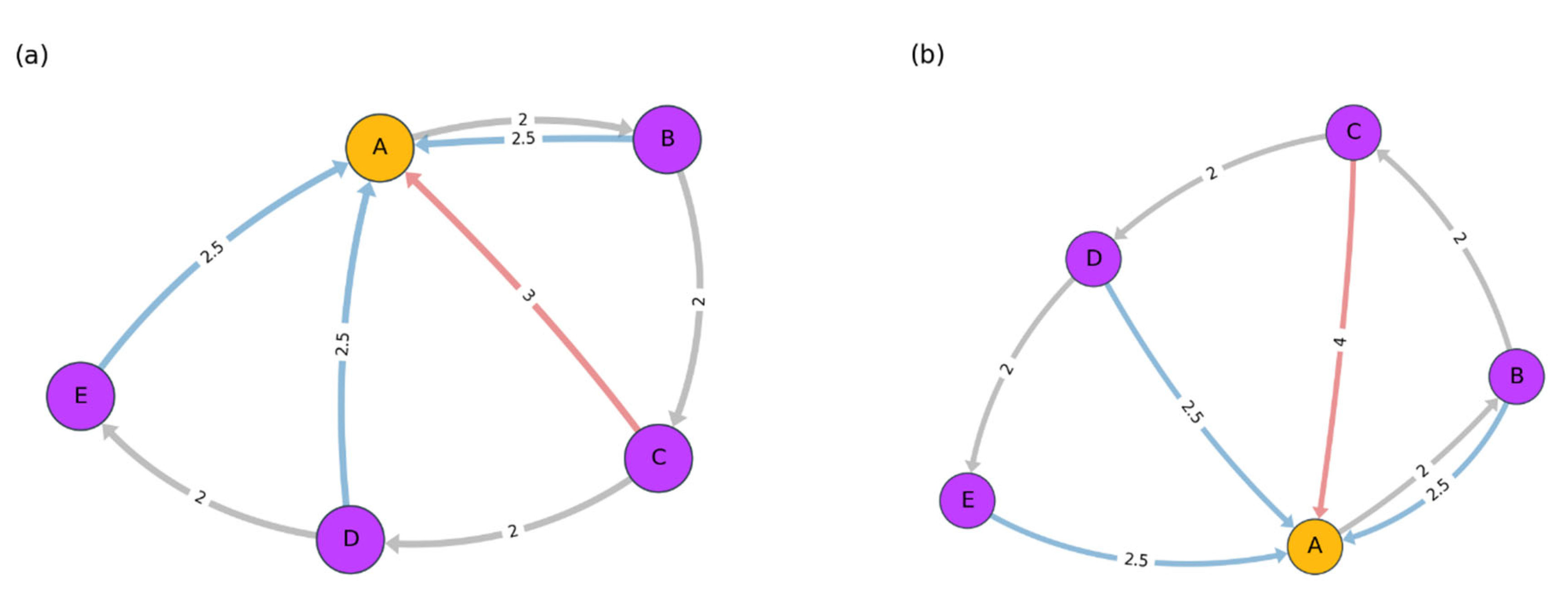
Intuitively, the longer the actual path is compared to the , the more is positive, and therefore path stays closer to the original vertex than one would expect from the maximum distance back to that starting point (Figure 2).

Figure 2.
Toy example for the simplified and modified Haantjes curvature. In both figures, and , represented by gray edges. Regarding the second quantity the value is represented by a red edge. The value of the path in (a) is and for (b) is . Hence, the path length in (a) is more curved and circulates in a smaller “radius” compared to the path length in (b).
Observe that, for our purposes, we have modified the Haantjes curvature by replacing the length of the chord with the maximum of the distances from each of the vertices to . This change enables us to estimate the amount of “effort” one has to exert in order to return to from each of the vertices . To distinguish between the length of the path denoted by and the maximum distance between the starting point and the other vertices in the path, we have chosen the distances to the first word and not the distances from the first word. This distinction is possible because the metric axioms are violated in our “distance” function, and this violation is particularly evident for the symmetry assumption. Another consequence is that we allow cases in which the path curvature is negative, in other words, where is smaller than the maximum distance from to .
Our modification also enables us to measure more types of paths than Haantjes curvature allows. Haantjes curvature is calculated only for simple paths, meaning paths in which the only edge that returns to the first vertex is the edge that connects the last vertex to the first. By contrast, because our simplified and modified Haantjes curvature considers the maximal distance back to the starting point, we are able to calculate curvature even when additional vertices in the path are connected by an edge to the first vertex—in other words, even if an elementary cycle is not obtained. We therefore cannot refer to the modified Haantjes curvature that we employ here as a discrete version of Ricci curvature. A final modification, which we have already mentioned, is our focus on actual rather than possible paths.
Next, we define the simplified and modified Haantjes–scalar curvature of a vertex v :
Definition 5.
Let be a vertex in a graph . Then the simplified and modified Haantjes–scalar curvature of is defined as
wheredenotes the paths that are starting at vertex.
The curvature has two free parameters. The first parameter controls the percentage of the existing edges of a given path, so is calculated only if at least X percent of the consecutive words in are represented by a weight in the graph. In the analyses we present below, we use all the paths with at least one edge with a weight in the graph. We provide more details about this parameter in the Appendix A.
The second parameter is the length of the paths on which the that starts from vertex v is calculated. In the following analyses, will be calculated separately for paths having . We choose short path lengths so that we can focus on the correlation between and velocity for groups of words that are relatively close to the first word in the path. Note that for statistical reasons, we use the median and not the sum in our calculations of and in all of our statistical analyses.
4. Exploring the Measure
In this section we present an initial validation of our assumption that an attractive path is one that remains close to the starting word, and then we examine the relationship between attraction and Haantjes curvature. Next, we show that the attraction of a word based on the way people actually retrieve words is not explained by a greedy search. Finally, we examine the relationship between a word-based strategy search, which we measure by level of attraction, and accessibility to information stored in memory, which we measure by velocity.
4.1. Validation
This section consists of two parts. First, we propose an initial validation that a path defined as attractive by is a path that remains close to the starting word. Then, in order to show that does not collapse into , we examine the relationship between the original Haantjes–scalar curvature- and our simplified and modified Haantjes–scalar curvature . (See Appendix A for descriptive statistics of these two measures.)
To validate that expresses the extent to which a path remains close to the starting word, we consider two variables for each existing path . The first variable is the attraction of the path measured by , and the second variable is , which denotes the transition time from directly to . Note that the transition time from directly to or from directly to does not appear in the calculation of . We assume that a fast transition indicates that the words are semantically close, and on the basis of this assumption, we show that the more positive is—in other words, the more attractive the word—the the more quickly the subject makes the transition from directly to .
We control for frequency, since many studies have reported a strong correlation between frequency and accessibility between two adjacent words [26]. We also control for location, since there is a strong correlation between the average location of a word and the time it takes to transition to the next word in our task (see Appendix A).
The following analysis describes the relationship between the transition time from word i to word j, and the median for any path that starts at and ends at . In order to assess the effect of on , we constructed a set of networks in which the weights are determined by the “distance function” with two free parameters, window size (WS) and minimum number of subjects per edge (MS). Each network was set with a pair of WS and MS within the following ranges: WS = (1,2,…,9) and MS = (3,5,7,9,11,13,15,17,19,21). Given all possible combinations between WS and MS, we constructed a total of 90 networks. Note that all networks were built by the lists of words that the subjects provided. However, each network has a distinct set of weights since the weights of the edges are determined by the free parameters WS and MS. Namely, the weight is determined by the set of lists that has at least MS subjects who said the word i and then the word j when the maximal words in between i and j is at most WS words.
We examine the relationship on a large number of graphs to estimate the stability of the result for distances with different degrees of locality (WS) and power (MS). Then, for any actual path length k = 3 or 4, we calculate the and as follows:
- (a)
- For each edge (), if the number of paths of length k that started at and ended at was equal to or greater than a threshold = [10,20,30], we calculated the median of and the median of for all the paths of length k that started at and ended at .
- (b)
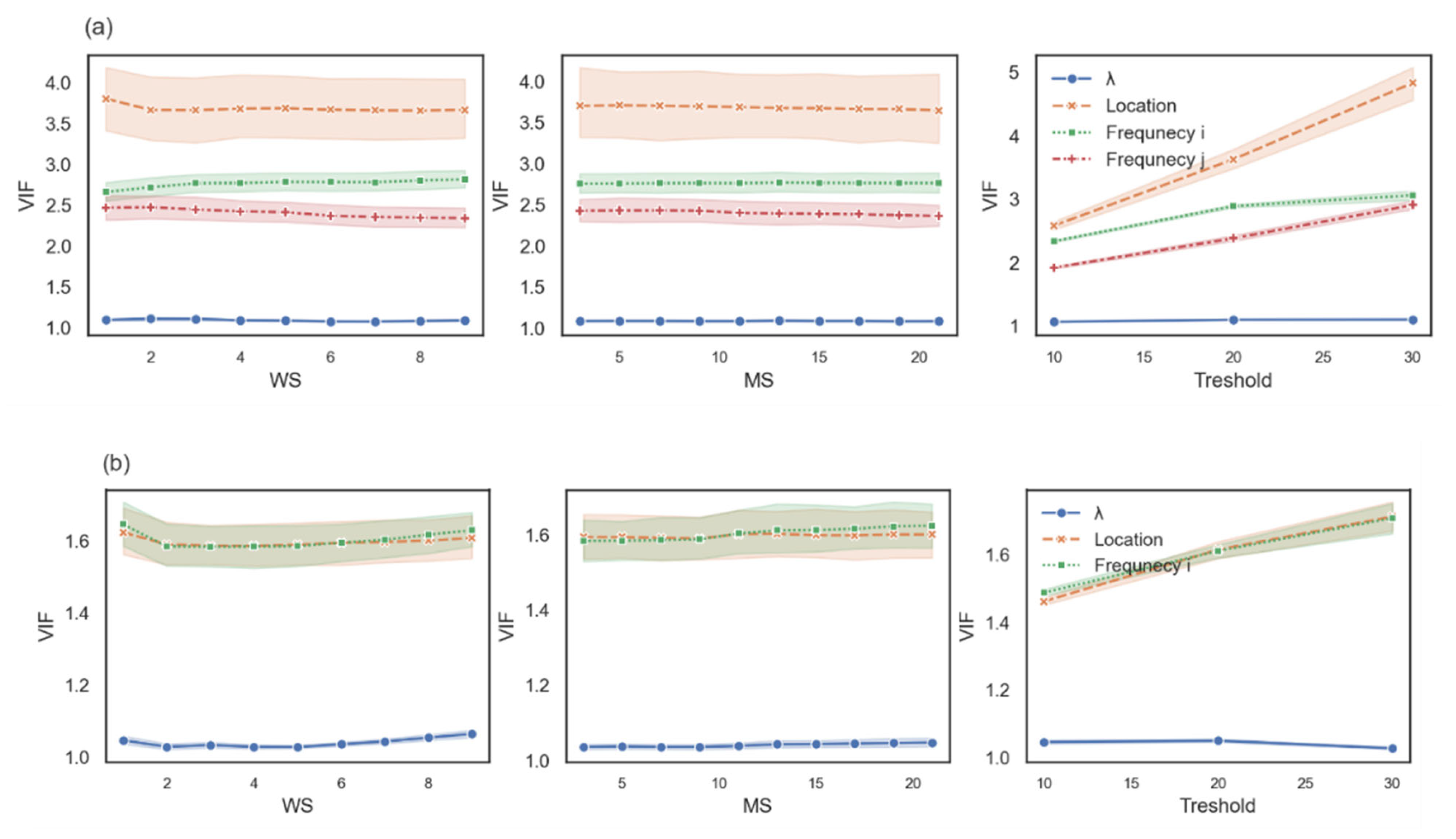
- For any possible combination among k, WS, MS, and the threshold, we ran a robust linear regression. To control the log-frequency of words i and j and the location of word i, we tested multicollinearity by computing the variance inflation factor (VIF) between them (Figure 3). VIF is computed for each variable as an indicator of multicollinearity, where VIF > 2.5 indicates considerable collinearity [27]. Since the VIF score of the location of word i and the log-frequency of words i and j were greater than 2.5, we ran two robust linear regressions using the statsmodels package in Python [28]. For those two models, the VIF of the variable were less than 2.5 (see Figure 3b,c). Additionally, , log-frequency, and word location were standardized via Z-score. The first model controlled the log-frequency and location of word I, and the second model controlled the log-frequency of word j and the location of word i.
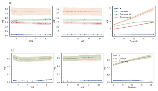
 Figure 3. The VIF score of each measure as a function of the free parameters. The variance inflation factor (VIF) score of all four independent variables is shown in row (a), the VIF score for a model with independent variable location, log-frequency i, and is shown in row (b), and the VIF score for a model with independent variable location, log-frequency j, and is shown in row (c).
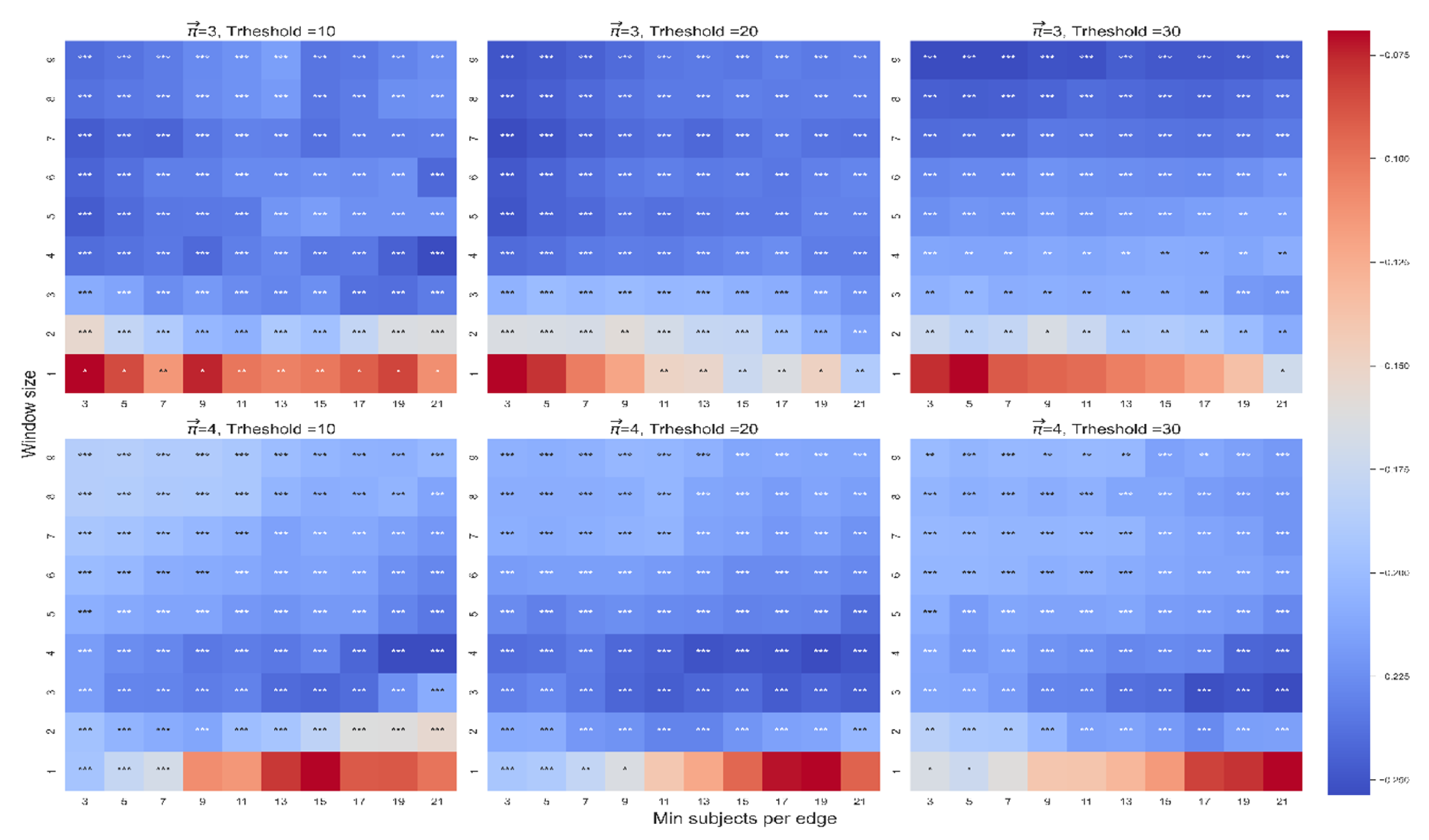
In both models we found a robust effect of on (see Figure 4 for the first model and the Appendix A for the second model). We found no robust interaction between and mean location in either model and no robust significant effect of either type of frequency or location on (See the Appendix A for supplementary descriptive statistics and for other results). In sum, our analysis suggests that indeed captures how close a path remains to the starting word.

Figure 4.
The beta coefficient between and in the first model. The color highlights the sign and magnitude of the beta coefficients. A blue cell indicates a negative beta, and a red cell indicates a positive beta. The number of stars indicates the level of significance (* p < 0.05. ** p < 0.01. *** p < 0.001). In each heatmap, the x-axis indicates the range of WS, and the y-axis indicates the range of MS. Each plot presents a different combination of the free parameters of path length (3 or 4) and threshold (10, 20, or 30).
4.2. Comparison between and
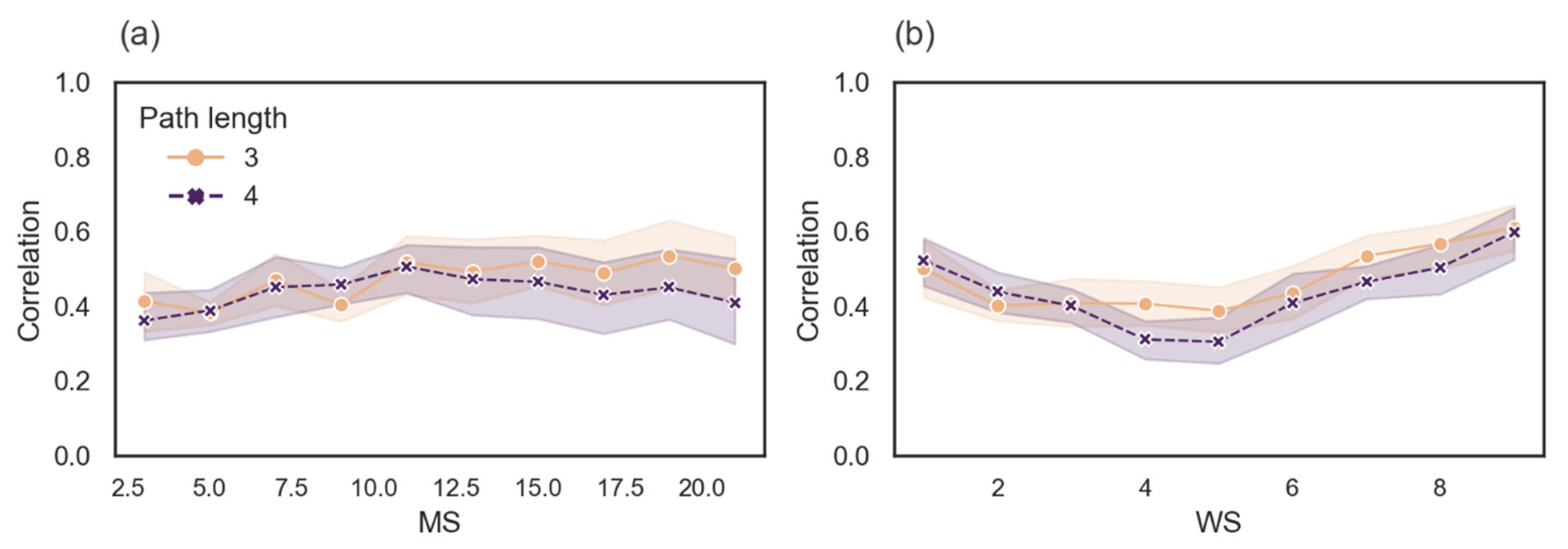
Next, we examined the relationship between and by performing a Spearman correlation test. We performed all the analyses on the set of vertices that received a value for each of the curvature measures. Additionally, we tested the correlation between the two measures on a range of parameters of the distance function. The first parameter, minimal subjects per edge (MS), comprises the values (3,5,7,9,11,13,15,17,19,21). The second parameter, window size (WS), comprises the values (1,2,…,9), maximal words that determine the distance between a given pair of words. Finally, since and are measures of path curvature, we examined the curvature for path length larger than 2 (edge), namely 3 or 4 (see Figure 5).
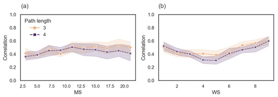
Figure 5.
Spearman correlation between and Graph (a) shows the correlation between and as a function of MS, and graph (b) shows the correlation between and as a function of WS.
The average correlation between and for length 3 is 0.47 (SD = 0.12), and the coefficient of determination is 0.22, meaning that only 22% of the data fits the line on average. For length 4 the average correlation is 0.43 (SD = 0.13), and the coefficient of determination is 0.18, meaning that only 18% of the data fits the line on average. In addition, the correlations as a function of MS and WS hardly change. In sum, we show that that does not collapse into the measure.
4.3. Greedy Search vs. Attention-Oriented Search
We argue that the level of attraction of word S as measured by expresses an attention-oriented search, which means that the agent sustains attention to S and therefore continues to sample words in S’s vicinity. An alternative explanation is the greedy search: because many words are close to S and close to each other, the agent continues to sample words in S’s vicinity because it is “easy” to retrieve those words. The difference between these two types of searches lies in the role of the first word in the path. An attention-oriented search assumes that the agent keeps paying attention to S. This condition is unnecessary in a greedy search, where the transition between words that are adjacent to S is explained by the high probability of remaining in S’s vicinity, even if the agent is paying attention to S.
This section examines whether -measured attraction produces a pattern for actual paths that is different from the pattern for the possible path of a random walker on the graph, which represents a greedy search. We will show that the attraction of a word based on the way people actually retrieve words is not explained by a greedy search.
4.3.1. Measure
We now introduce the process by which we created random walker paths. Those paths are based on the conditional probability of the present word, which dictates the movement from one vertex to another on the graph. For a word on a random-walker path, is calculated as follows:
Each path represents a possible path on the graph by a random walker. The weight of for the path is the probability of the path denoted by . Finally, we normalize the product of and with the sum of the probabilities of all the paths starting with v. We perform this process for any paths of length 3 or 4. Additionally, we limit the possible paths to ones that are non-repetitive; for example, dog–dog–dog is not taken into account even though there is a positive probability from dog to dog.
This procedure allows us to calculate for paths in which the transition from one vertex to another takes only the current word into account—in other words, for paths in which the first word “attracts” only the word that follows immediately, and not words that come later in the sequence. We aim to show that cannot be explained by .
4.3.2. Results
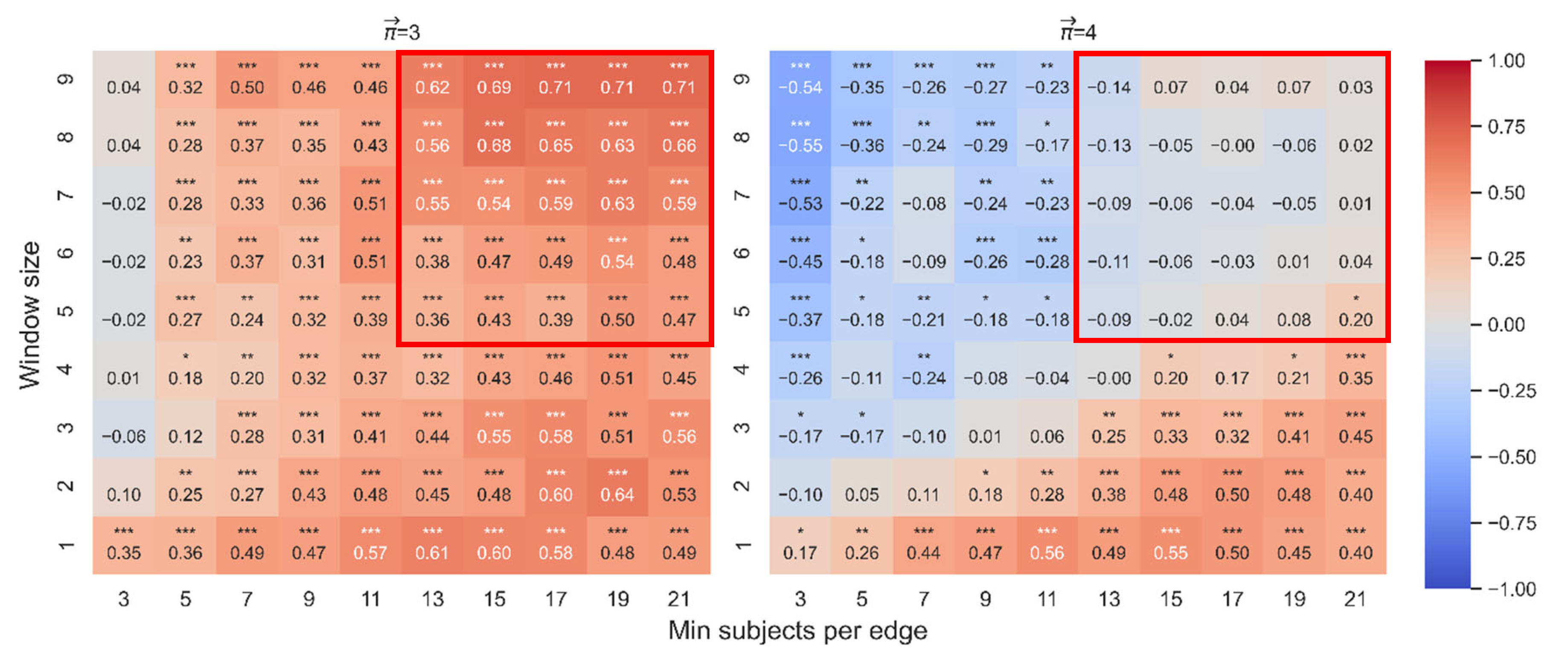
We performed a Spearman correlation test between the distributions of and for all vertices that received a value for . Additionally, we tested the correlation on a range of two parameters of the distance function. The first parameter, minimal subjects per edge (MS), comprises the values (3,5,7,9,11,13,15,17,19,21). The second parameter, window size (WS), comprises the values (1,2,…,9), maximal words that determine the distance between a given pair of words (see Figure 6).
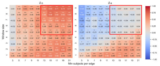
Figure 6.
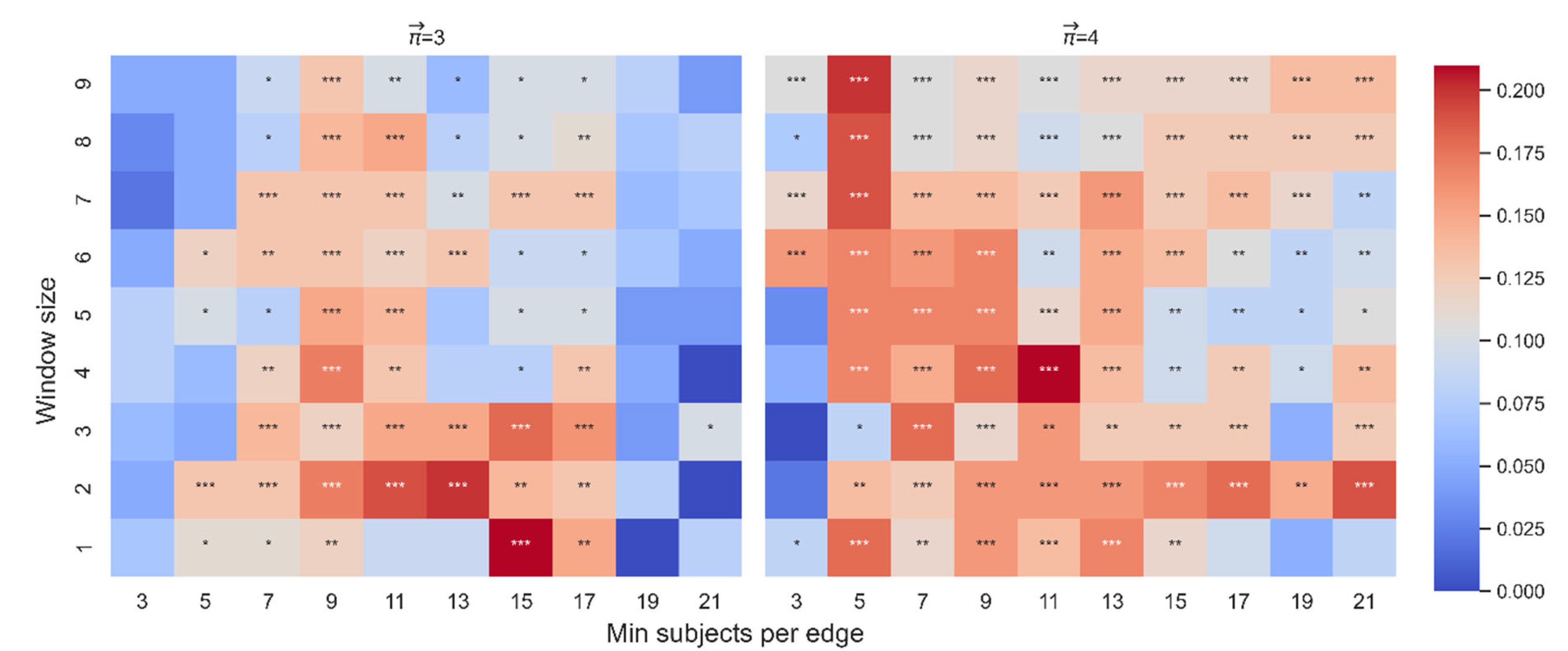
Spearman correlation between and . The color reflects the sign and magnitude of Spearman coefficients. A blue cell indicates a negative correlation; a red cell indicates a positive correlation. The number of stars indicates the level of significance (* p < 0.05. ** p < 0.01. *** p < 0.001). The left heatmap shows the results for paths of length 3, and the right heatmap does the same for paths of length 4.
For paths of length 3, the mean correlation is 0.41 (median = 0.45, SD = 0.18). This result indicates that the fitted line explains between 0% and 51% of the data, and the mean is 17%. For paths of length 4, the mean correlation is 0.01 (median = −0.03, SD = 0.27). This result indicates that the fitted line explains between 0% and 31% of the data, and the mean is 4%.
For paths of length 3, there exists a correlation between and that becomes stronger as the weight of the edges increases based on the number of people who retrieve word A and then word B. This relationship is reflected by the area outlined in red on the left heatmap in Figure 6. For paths of length 4, however, the correlation is weak or non-existent. As demonstrated by the outlined area on the right heatmap in Figure 6, the correlation disappears completely for the range of graphs in which the weights are based on a large number of people who retrieve word A and then word B.
In sum, the relationship between the measures is stronger for path length 3 because the degrees of freedom are relatively low; however, when the paths are increased to a length of 4, the correlation almost disappears. These findings allow us to establish an empirical distinction between the greedy search and the attention-oriented search. Earlier in this paper, we presented a theoretical distinction between the two types of searches: for the greedy search, path length contributes negatively, whereas for the attention-oriented search, path length contributes positively. Here we have shown empirically that does not collapse into , which calculates the curvature based on random paths that express a greedy strategy.
In the next section, we will examine the relationship between attraction-based actual paths and accessibility to information stored in memory as we control for attraction-based random walker paths.
5. Case Study: Attraction and Accessibility
This section demonstrates a possible use of the attraction measure through a case study that focuses on a semantic network. To validate our measure psychologically, we examined the relationship between velocity and attraction. Retrieval velocity is one way to estimate the extent to which information is accessible to the subject: the greater the velocity, the greater the degree of accessibility. We focused on whether a high level of attraction enables faster access to the words that remain in the attractive word’s vicinity. Stated differently, if an agent sustains attention to word S and S creates a semantic context, does the agent retrieve additional words from that context more quickly? We hypothesized that the correlation between the level of a word’s attraction and the velocity of the agent’s retrieval is negative: the greater the level of attraction, the less time it takes to move from one word to another.
5.1. Measuring Velocity
For any vertex and all the paths , let be the set of paths where is the l-th vertex in the path p. We then calculate the average time that it takes to move within the set of vertices on paths of length k = 3 or 4 for which the attraction has been calculated. We compute the velocity of vertex in as follows:
Here it is worth clarifying the fundamental differences between velocity and attraction.
The attraction takes as its input the weights of the graph and calculates two quantities. The first is , which represents the sum of the weights of the consecutive words in the path. The second is , which expresses the maximum distance back to the first word in a path. Note that for a constant , the contribution of is positive. As quantity increases, so does the degree of attraction. The distance from to is defined as the median of the transitions in window X with a minimum of Y subjects who made this transition, and this means that a slow transition between a pair of words contributes positively to the degree of attraction. By contrast, the velocity of the set of words in a path of length k, which starts with word v, is directly calculated by the amount of time that it takes to traverse the set of words. We say that vertex v is characterized by high velocity if the median times of the paths starting with v are very fast. Here, unlike the case with attraction, the contribution of slow transition is negative: the slower the transitions of the paths, the lower the velocity of vertex v. Since both attraction and velocity are based on the same lists of words participants produced, we must rule out a trivial relationship between them. We explain this process below.
5.2. Results
Spearman correlation was calculated between attraction, based on paths of length 3 or 4, and velocity, measured by Equation (7). The correlation was calculated for a range of parameters of the distance function: minimal subjects per edge (MS) (range: 3,5,7,9,11,13,15,17,19,21) and window size (WS), or the maximum number of words between a given pair of words that constitute an edge (range: 12,…, 9).
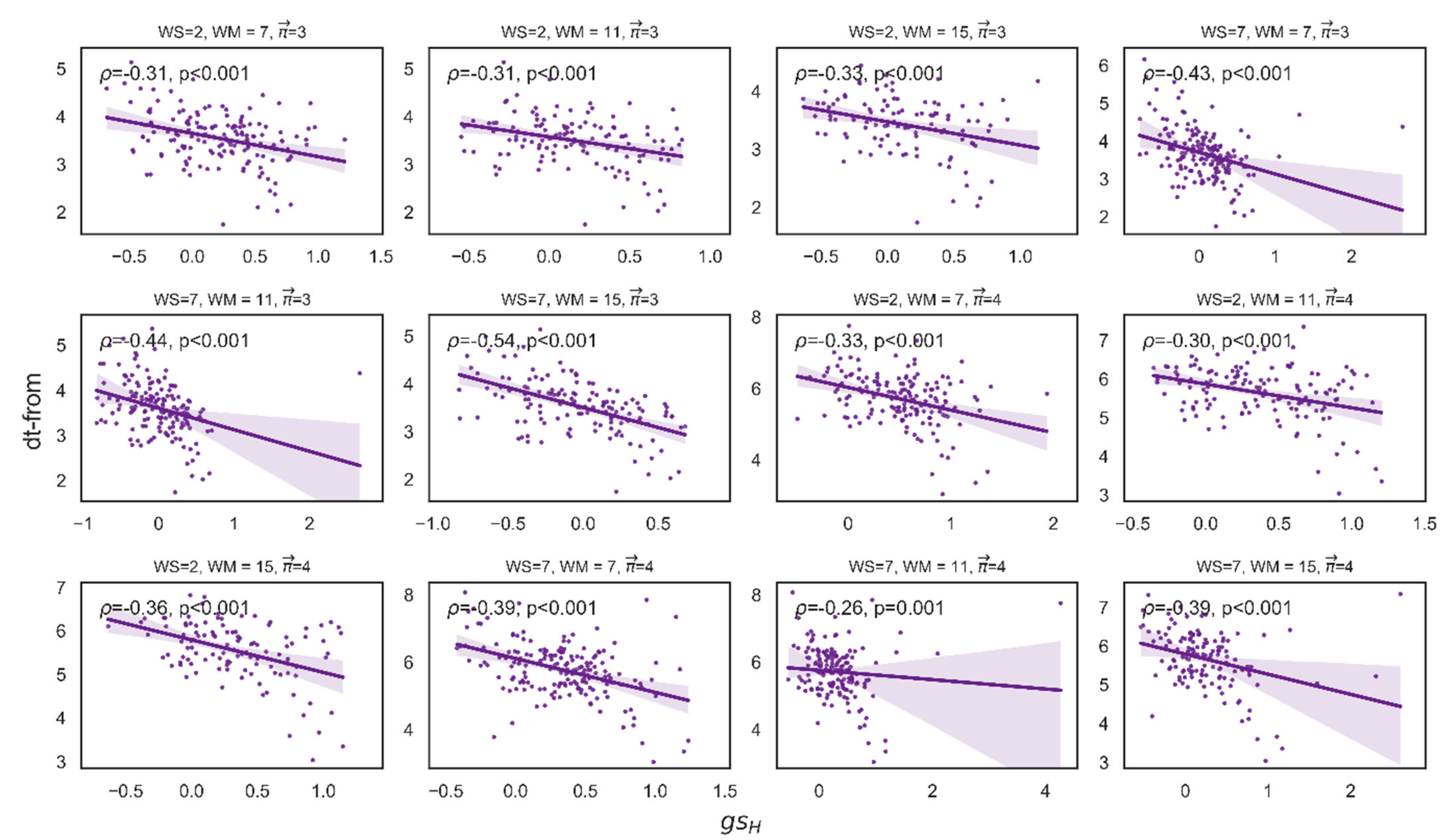
For length 3, out of 90 correlations between attraction and velocity, 88 were significant. For length 4, 89 were significant (see Figure 7). Figure 8 presents some examples of the correlation between attraction and velocity for a set of parameters WS: 2,7 and MS: 7,11,15 and length k = 3,4.
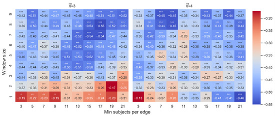
Figure 7.
Spearman correlation between attraction ( and velocity (dt-from). The color highlights the sign and magnitude of Spearman coefficients. A blue cell indicates a negative beta; a red cell indicates a positive beta. The number of stars indicates the level of significance (* p < 0.05. ** p < 0.01. *** p < 0.001). The left heatmap is for paths of length 3, and the right heatmap is for paths of length 4.
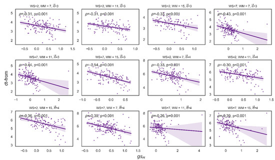
Figure 8.
Some examples of the Spearman correlation between attraction ( and velocity (dt-from). These are examples of the correlation for a set of parameters WS: 2,7 and MS: 7,11,15, where the x-axis denotes attraction, and the y-axis denotes velocity.
5.3. Testing Triviality
Since both attraction and velocity are based on the same lists of words participants produced, we must rule out a trivial relationship between them. To do this, we compare actual paths with paths we create by shuffling lists of words from actual paths. It is important to note that these shuffled paths preserve the frequency and word count of actual paths. Our goal is to show that the correlation between attraction and velocity is significantly higher for actual paths than for shuffled paths.
Let us now estimate the correlations between attraction measured by and velocity measured by dt-from (Equation (7)) for shuffled paths. Let be a set of paths and be an actual path of subject , where contains the sequence of word to word and the length of is . First, let be a set of where is a random order of the path of subject . Second, let such that the distances between the vertices are defined by Third, calculate and df-fromr based on and . Fourth, let denote the correlation between and df-fromr. The correlation can be generated by repeating steps one through four times, and as a result denotes the set of correlations obtained from the random orders. Finally, the distribution of defines the null hypothesis, and the statistical significance is the probability of obtaining the real correlation, obtained from the actual order, which is at most 5% at the null hypothesis.
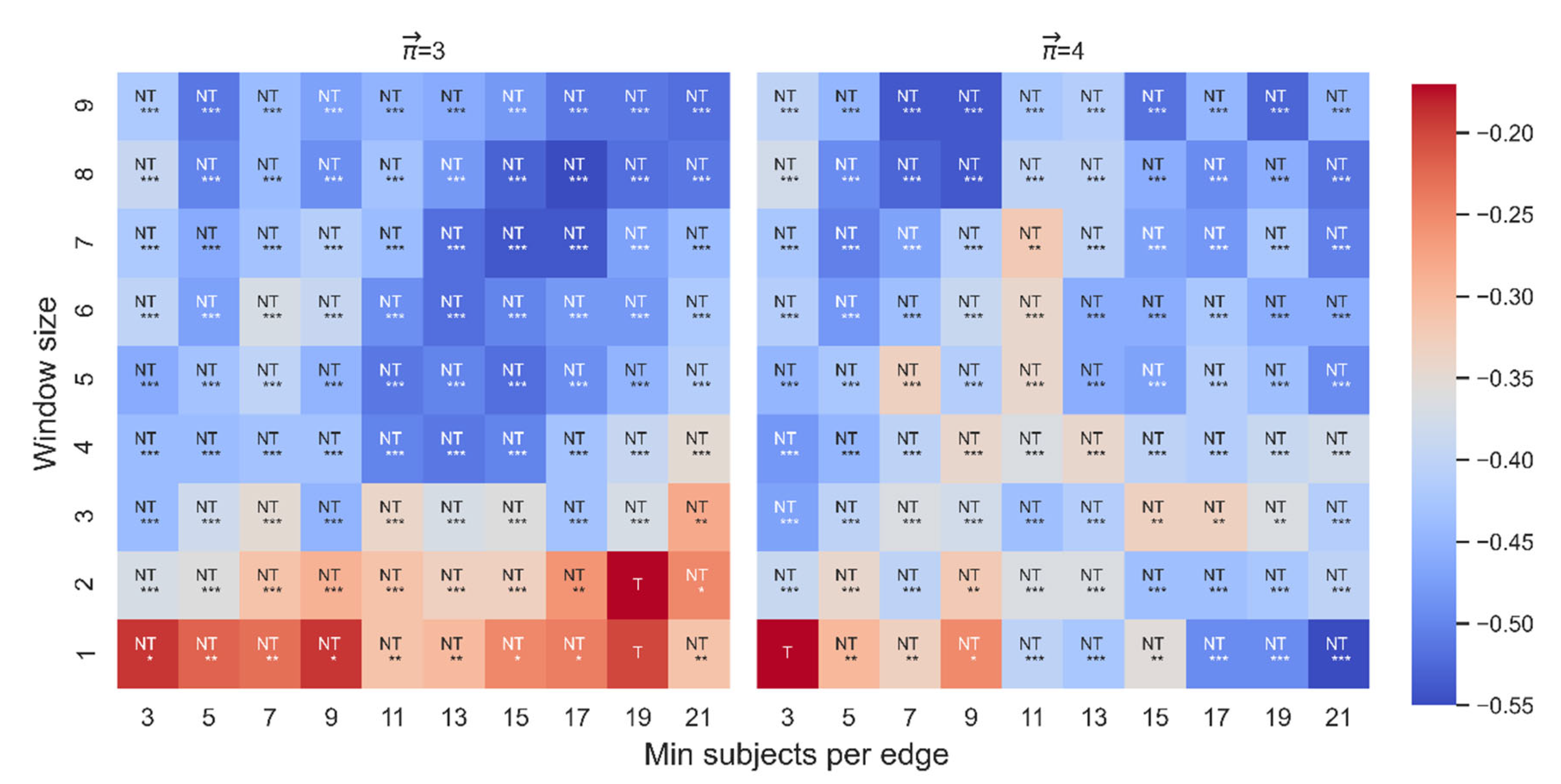
Triviality was tested for any significant correlation between and dt-from, given the following range of parameters of the distance function: WS: [1,2,…,9] and MS: (3,5,7,9,11,13,15,17,19,21). None of the significant correlations between and dt-from were trivial for either length 3 (88/90) or length 4 (89/90) (see Figure 9).
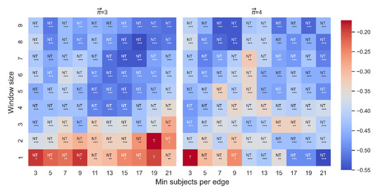
Figure 9.
Triviality test for the Spearman correlation between and dt-from. The color highlights the sign and magnitude of Spearman coefficients. A blue cell indicates a negative beta; a red cell indicates a positive beta. The number of stars indicates the level of significance (* p < 0.05. ** p < 0.01. *** p < 0.001). NT denotes that the correlation is non-trivial; T denotes that the correlation is trivial. The left heatmap is for paths of length 3, and the right heatmap is for paths of length 4.
5.4. Controlling for the Attraction-Based Random Walker and Average Location
Finally, we examine whether predicts dt-from even when controlling for attraction based on the random walker. We control, too, for the average location of the word, because word location maintains a positive correlation with dt-from (Figure 10). As the participant progresses through the retrieval process, the transition time between consecutive words increases, so words that tend to appear at the beginning of the list are characterized by a higher retrieval speed than words that come later. Controlling for word location allows us to examine whether a word’s attractiveness depends on the word’s location or whether attractive words facilitate retrieval even as the stream of associations progresses and the subject experiences increasing difficulty in retrieving other words. Figure 10a shows the correlation between average location and dt-from for all the words, and Figure 10b illustrates the correlation between them for a set of words that receives a value for (WS = 5 and MS = 11). Note, the single example presented above (WS = 5 and MS = 11) is consistent with the results provided by any other combination between WS and MS. The average correlation between average location and dt-from is 0.45 for path length 3 and 0.55 for path length 4.
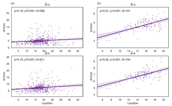
Figure 10.
Spearman correlation between average location and dt-from. The graphs in column (a) denote the correlation between average location and dt-from for paths of length 3 or 4, for all vertices that receive a positive value for average location and dt-from. The graphs in column (b) denote the correlation between average location and dt-from for paths of length 3 or 4, for vertices that receive a positive value for for WS = 5 and MS = 11.
To achieve this aim, we ran a robust linear regression for all pairs of parameters MS and WS in which the correlation between and dt-from was not trivial. We analyzed the results with two robust linear regressions using the statsmodels package in Python [27] to assess the effect of (continuous), (continuous) and average location (continuous) on dt-from. The first model assesses the effect for paths of length 3, and the second model assesses the effect for paths of length 4. Our models for this analysis were as follows:, where is the dependent variable dt-from for word i, represents the fixed effect , represents the fixed effect , represents the fixed effect of average location, and represents the residuals. We considered all possible interactions, and we standardized , , and average location via z-score. We ran each model for the range of parameters of the distance function as follows: WS: (1,2,…,9) and MS: (3,5,7,9,11,13,15,17,19,21).
As a first step, we tested multicollinearity by computing the variance inflation factor (VIF). The mean VIF of average location, , and was below 2.5, which means that the variables are not correlated (for more details, see Appendix A).
In connection with the model which assessed the contribution of and location for paths of length 3, out of 88 non-trivial and significant correlations between and dt-from, only 7 betas were significant (Figure 11). However, the effect of the interaction between and average location on dt-from was significant in 55 cases (Figure 12). The results show that the interaction yields an effect more stable than the effect of alone. In addition, since the purpose of this section is to examine the stability of the correlation between and dt-from controlled by and average location, here we report the effect of and the effect of the interaction of with average location so that we can account for the possibility that changes depending on the position of the word. See Appendix A for this analysis on .
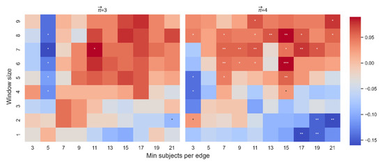
Figure 11.
Beta coefficient between and dt-from. The color highlights the sign and magnitude of the beta coefficients between and dt-from. A blue cell indicates a negative beta; a red cell indicates a positive beta. The number of stars indicates the level of significance (* p < 0.05. ** p < 0.01. *** p < 0.001). The left heatmap is for paths of length 3, and the right heatmap is for paths of length 4.
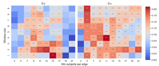
Figure 12.
Beta coefficient for the effect of the interaction between and average location on dt-from. The color highlights the sign and magnitude of the beta coefficients between and dt-from. A blue cell indicates a negative beta; a red cell indicates a positive beta. The number of stars indicates the level of significance (* p < 0.05. ** p < 0.01. *** p < 0.001). The left heatmap is for paths of length 3, and the right heatmap is for paths of length 4.
In connection with the second model, which assessed the effect for paths of length 4, out of 89 non-trivial and significant correlations between and dt-from, 29 beta were significant (Figure 11). The effect of the interaction between and average location on dt-to was significant in 82 cases (Figure 12). See Appendix A for the effect of on dt-from and the effect of the interaction between and location on dt-from.
5.5. Model Comparison
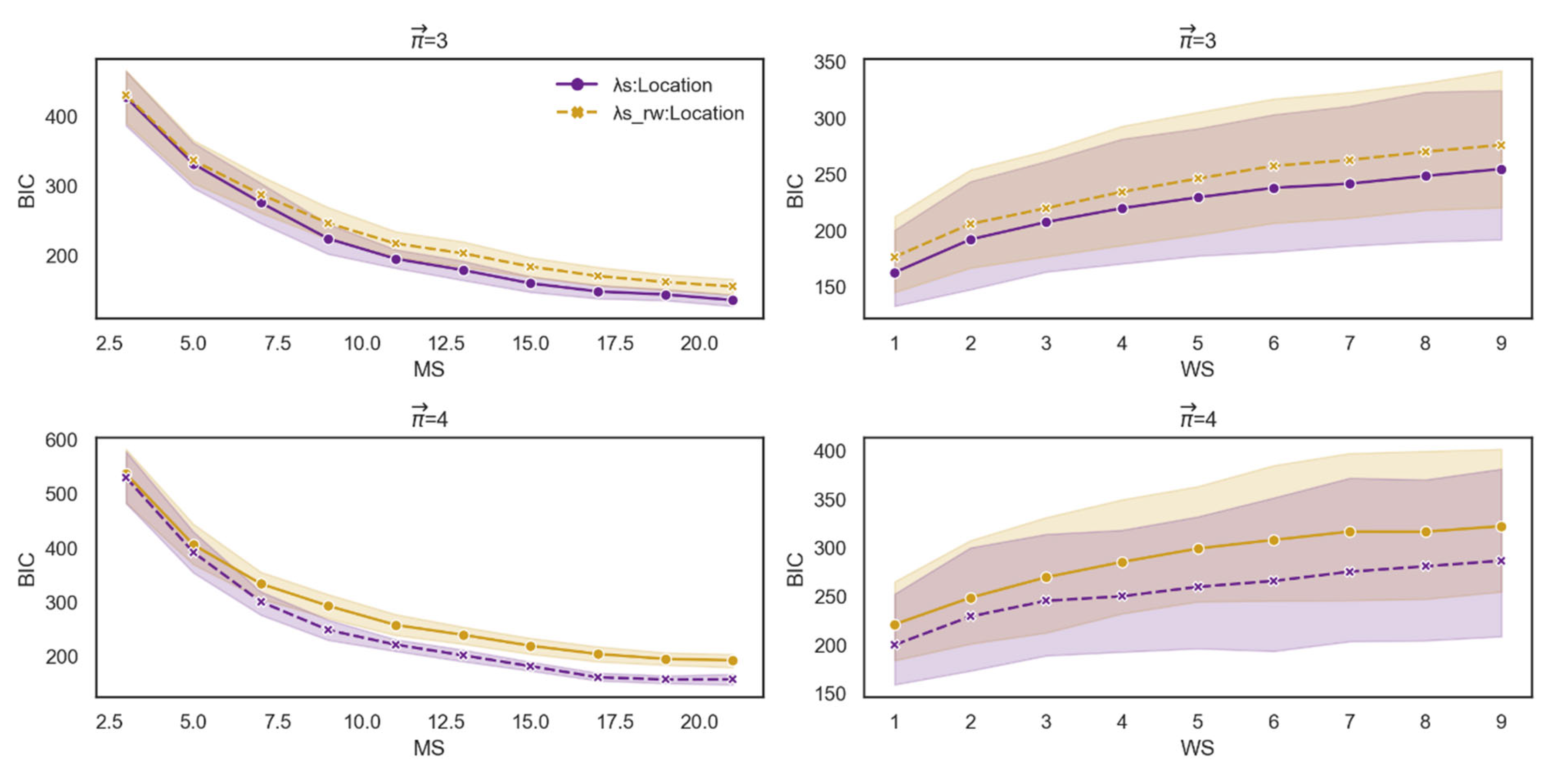
Finally, we constructed two bivariate models. The first tests the effect on dt-from of the interaction between attraction-based actual paths and average location. The second tests the effect on dt-from of the interaction between the attraction-based random walker and average location. Using the Bayesian information criterion (BIC) and the Akaike information criterion (AIC), we evaluated each model’s performance for a range of MS and MS values. We considered a lower BIC/AIC to represent the data better, and the results were robust. The interaction between attraction-based actual paths and average location yielded better results than the attraction-based random walker model (Figure 13). The results of AIC were consistent with BIC (see Appendix A for more details). That is, the model based on a random walker, which necessarily ignores the possibility that the first word affects the retrieval of the following set of words, is weaker than the model that takes into account the possibility that the first word affects the continuing retrieval of the following set of words.

Figure 13.
BIC score for each measure as a function of WS and MS. The first row denotes the BIC score for each measure as a function of WS and MS for path length 3. The second row denotes the BIC score for each measure as a function of WS and MS for path length 4.
6. Discussion and Conclusions
This paper introduces a novel geometric tool to investigate search strategies in memory. More specifically, we propose a measure based on Haantjes–Ricci curvature to determine how an agent searches for information related to a chosen word. A greater path curvature indicates a greater tendency to retrieve upcoming words in the semantic vicinity of the starting word, which means that the upcoming words remain related to the first word’s semantic context. While other measures in the literature have been limited to relationships between pairs of words, our novel measure can examine relationships within sets of words as well. As a result, it offers the opportunity to examine the effect of a word on the continuing retrieval process beyond the next word. In this regard, our word-based strategy is a novel proposition. From a cognitive perspective, it differs from other models in its assumption that different words attract different levels of attention and that, as a result, different words will have different effects on continuing retrieval. Unlike previous approaches (e.g., [6, 7]), which assume that the present word affects only the next word, our approach captures a word’s effect on the retrieval of a set of several words.
We investigated the proposed measure in four different but complementary ways. First, we verified that it does not simply reduce to Haantjes curvature. Second, we checked that the measure expresses the extent to which a path remains close to the starting word. Third, we showed that the way people actually retrieve words cannot be explained by a greedy search, which attributes path curvature to the ability of the first word to engage the agent in a large set of interconnected words, whether or not the agent sustains attention to that first word. Our finding supports the notion of an attention-based search, which attributes path curvature to the agent’s continued attention to the original word. Finally, we showed a link between our measure of attraction and accessibility to information stored in memory. Starting with the assumption that the greater the velocity, the greater the degree of accessibility, we demonstrated a significant and non-trivial relationship between attraction ( and accessibility to information stored in memory. A higher correlated with a higher velocity. When we controlled for a greedy search and word location, we found a significant interaction between word location and . Finally, we found that the attention-oriented search predicts velocity better than the greedy search. This finding reinforces our assumption that the search strategy that predicts the velocity of a given set of words rests on the relationship between the starting word and its following set. This claim is consistent with our interpretation that the relationship between a word and its subsequent set of words expresses the subject’s ability to sustain attention to the starting word. More simply, we believe that the agent searches most efficiently by “seeing” the upcoming words in light of the starting word. Path-based analysis makes it possible to examine different aspects of sustained attention on the serial retrieval process.
This study’s limitations suggest topics for further research. To highlight the shift from an edge-based to a path-based approach, future research might focus on the relationship between our measure and different types of Ricci curvature, such as Ollivier, Menger, and Forman [9,10,12]. Additionally, as we have shown, word location plays an essential role in the relationship between attraction and velocity ( and dt-from), and further research might take up the importance of this mediator. Finally, future studies might use a discrete notion of Ricci flow to elucidate how the first word determines the search strategy for the following set of words. An attractive word S keeps upcoming words in its environment, but if S changes the relationships between other words, those relationships must be passing through S’s semantic prism. Ricci flow offers a promising way to measure the extent to which a word changes the semantic relationships in its environment. Elucidating the connection between a word’s attractive and prismatic functions will strengthen the claim that a path-based attraction measure does indeed express the attraction of the first word in the path.
Author Contributions
Conceptualization, H.C., Y.N., P.M.N., A.M. and E.S.; methodology, H.C. and Y.N.; formal analysis, H.C., Y.N., P.M.N., J.J. and E.S.; statistical analysis, H.C.; writing—original draft preparation, H.C.; writing—review and editing, H.C., J.J., A.M. and E.S.; visualization, H.C.; supervision, A.M. and E.S. All authors have read and agreed to the published version of the manuscript.
Funding
This research was partially supported by the German-Israeli Foundation [grant I-1514-304.6/2019 to Emil Saucan and Jürgen Jost] and the Israel Science Foundation [grant 1471/20 to Anat Maril].
Institutional Review Board Statement
The study was conducted in accordance with the Declaration of Helsinki, and approved by the ethics committee of the Department of Psychology at the Hebrew University of Jerusalem (15 November 2021).
Informed Consent Statement
Informed consent was obtained from all subjects involved in the study.
Data Availability Statement
All of the Python code and raw data material are publicly available via OSF (https://osf.io/w36tc/, 1 June 2022).
Acknowledgments
This research was partially supported by the Israel Science Foundation (grant 1471/20 to Anat Maril) and the German–Israeli Foundation (grant I-1514-304.6/2019 to Emil Saucan and Jürgen Jost).
Conflicts of Interest
The authors declare no conflict of interest.
Appendix A
This Appendix includes the following analyses: (1) descriptive statistics of and , (2) additional results for Section 4, validating the novel measure via the assumption that expresses the extent to which the first word in the path attracts the upcoming words, and (3) additional results for Section 5, focusing on further results regarding the linear regression between attraction and accessibility.
- 1.
- Descriptive Statistics
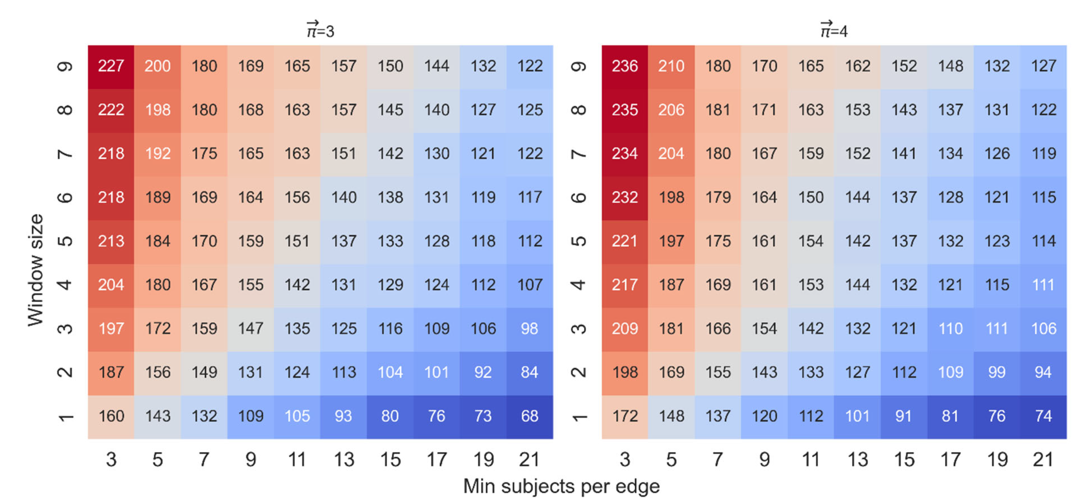
Figure A1 demonstrates a power-low-like distribution of the frequencies of the words. Figure A2 illustrates the number of vertices that receive a value for paths of lengths 3 or 4, with the parameter P set to . Each cell in Figure A2 represents the number of vertices for a pair of parameters MS = (3,5,7,9,11,13,15,17,19,21) and WS = (1,2,…,9). It is easy to see that with a greater WS and a lower MS, the number of vertices increases. However, the price of a low MS is the determination of some distances by a small number of subjects and the disproportionate effect on those distances of extremely fast or extremely slow transitions.

Figure A1.
The pie chart on the right presents the empirical cumulative distribution of word frequency, and the graph on the left presents the percentage of words belonging to the following frequency ranges: (1) 0–5 (2) 6–15 (3) 16–30 (4) 31–60 (5) 61–100 (6) 101–500 (7) >500.
Figure A1.
The pie chart on the right presents the empirical cumulative distribution of word frequency, and the graph on the left presents the percentage of words belonging to the following frequency ranges: (1) 0–5 (2) 6–15 (3) 16–30 (4) 31–60 (5) 61–100 (6) 101–500 (7) >500.
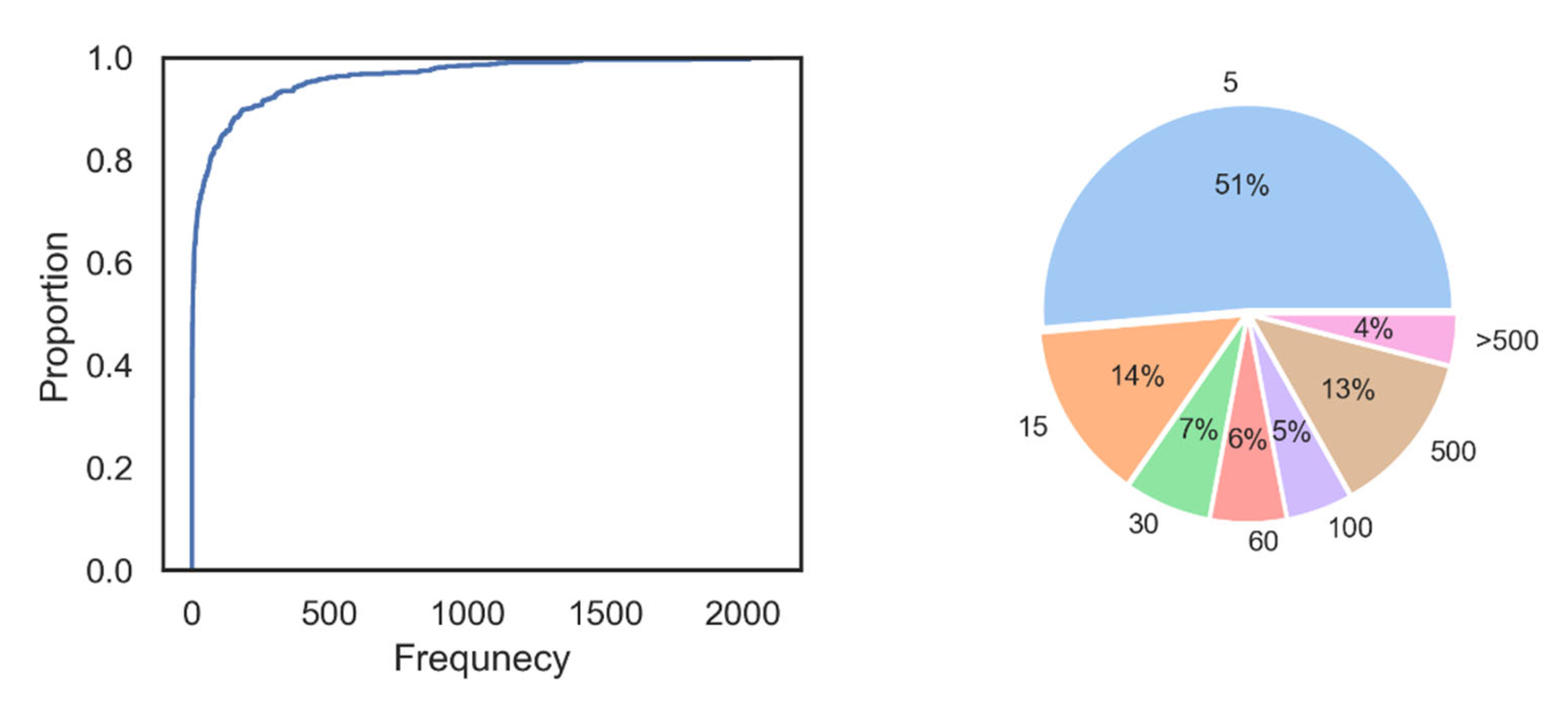

Figure A2.
Each cell represents the number of vertices that receive a value for the pair of parameters MS (minimum subjects per edge) and WS (window size). The x-axis denotes the range of MS values, and the y- axis denotes the range of WS values. The color highlights the number of vertices. Bluer cells indicate a lower number of vertices; redder cells indicate a higher number of vertices. The left heatmap is for paths of length 3, and the right heatmap is for paths of length 4.
Next, Figure A3 illustrates examples of the distribution of and for paths of length 3 or 4, as a function of the following WS and MS values: (WS, MS) = [(2,5),(3,13),(9,5),(9,13)]. The number of vertices with a value ranges from 116 to 210, where P is greater than 0% (for descriptive statistics, see Table A1).
Figure A3.
Eight examples of the distribution of and for a set of parameters (WS, MS) = [(2,5), (3,13), (9,5), (9,13)] and length () = 3,4. The x-axis denotes the curvature values.
Figure A3.
Eight examples of the distribution of and for a set of parameters (WS, MS) = [(2,5), (3,13), (9,5), (9,13)] and length () = 3,4. The x-axis denotes the curvature values.
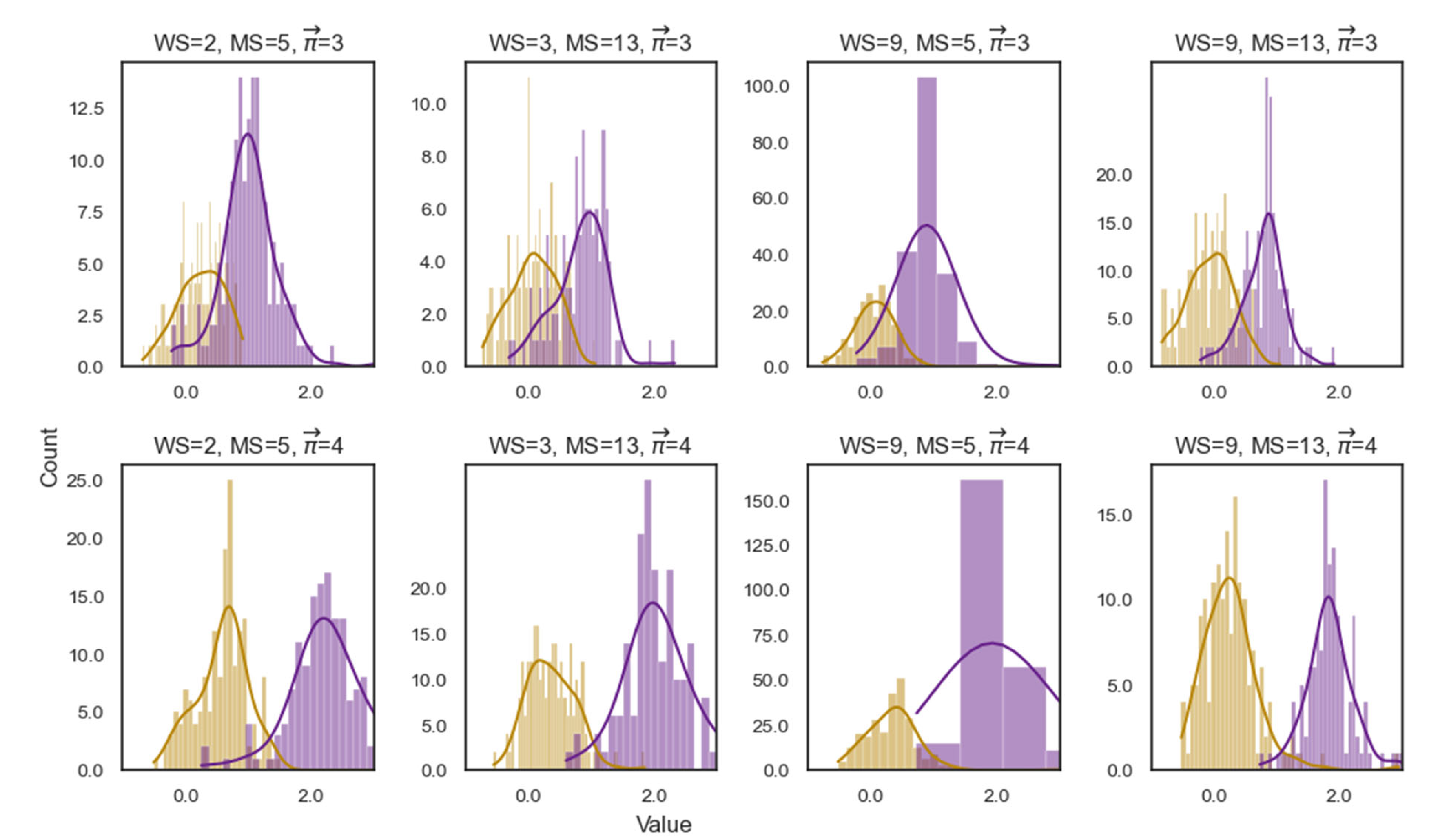
As can be noted in Figure A3 and Table A1, in all cases the minimum of is negative, which indicates that is smaller than the maximum distances from to These cases constitute a violation of the metric axioms.

Table A1.
Descriptive statistics for and for path length = 3 or 4. N indicates the number of vertices with a value. (WS, MS) denotes the free parameters of the distance function; we calculated on the basis of distance.
Table A1.
Descriptive statistics for and for path length = 3 or 4. N indicates the number of vertices with a value. (WS, MS) denotes the free parameters of the distance function; we calculated on the basis of distance.
| Type | (WS, MS) | Path Length | N | Mean | Median | S.D | Min | 25% | 75% | Max |
|---|---|---|---|---|---|---|---|---|---|---|
| (2,5) | 3 | 162 | 1.01 | 1 | 0.45 | −0.22 | 0.78 | 1.22 | 3.09 | |
| (3,13) | 3 | 107 | 0.83 | 0.87 | 0.42 | −0.31 | 0.6 | 1.12 | 2.33 | |
| (9,5) | 3 | 203 | 1.03 | 0.9 | 1.21 | −0.23 | 0.73 | 1.04 | 15.79 | |
| (9,15) | 3 | 130 | 0.78 | 0.83 | 0.33 | −0.22 | 0.57 | 0.97 | 1.92 | |
| (2,5) | 4 | 162 | 2.35 | 2.24 | 0.77 | 0.26 | 1.97 | 2.64 | 6.02 | |
| (3,13) | 4 | 109 | 2.12 | 2.04 | 0.73 | 0.6 | 1.76 | 2.36 | 6.29 | |
| (9,5) | 4 | 203 | 2.22 | 1.94 | 2.5 | 0.73 | 1.7 | 2.18 | 35.08 | |
| (9,15) | 4 | 130 | 1.85 | 1.83 | 0.41 | 0.73 | 1.64 | 2.01 | 3.92 | |
| (2,5) | 3 | 156 | 0.25 | 0.27 | 0.36 | −0.68 | −0.02 | 0.54 | 0.91 | |
| (3,13) | 3 | 125 | 0.08 | 0.08 | 0.37 | −0.73 | −0.16 | 0.36 | 1.07 | |
| (9,5) | 3 | 200 | 0.07 | 0.07 | 0.42 | −0.77 | −0.13 | 0.26 | 4.22 | |
| (9,15) | 3 | 157 | −0.06 | −0.03 | 0.37 | −0.83 | −0.3 | 0.19 | 1.06 | |
| (2,5) | 4 | 169 | 0.6 | 0.65 | 0.46 | −0.5 | 0.34 | 0.86 | 3.41 | |
| (3,13) | 4 | 132 | 0.37 | 0.34 | 0.38 | −0.55 | 0.09 | 0.63 | 1.86 | |
| (9,5) | 4 | 210 | 0.36 | 0.37 | 0.57 | −0.53 | 0.08 | 0.54 | 6.16 | |
| (9,15) | 4 | 162 | 0.26 | 0.22 | 0.42 | −0.52 | −0.02 | 0.45 | 2.94 |
We tested Spearman correlation between the distributions of for path lengths 3 and 4 for a range of WS and MS values. We found a significant correlation between them (see Figure A4). The mean and median correlation are both 0.762, and the standard deviation is 0.03. For the mean is 0.79, the median is 0.78, and the standard deviation is 0.01.
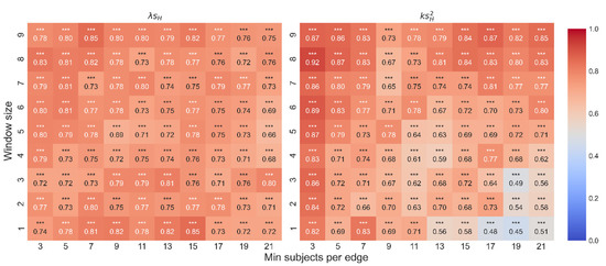
Figure A4.
We tested Spearman correlation between the distributions of / for path lengths 3 and 4 for a range of WS and MS values. The x-axis denotes the range of MS values, and the y-axis denotes the range of WS values. The color highlights the sign and magnitude of Spearman coefficients: blue cells indicate a negative beta; red cells indicate a positive beta.

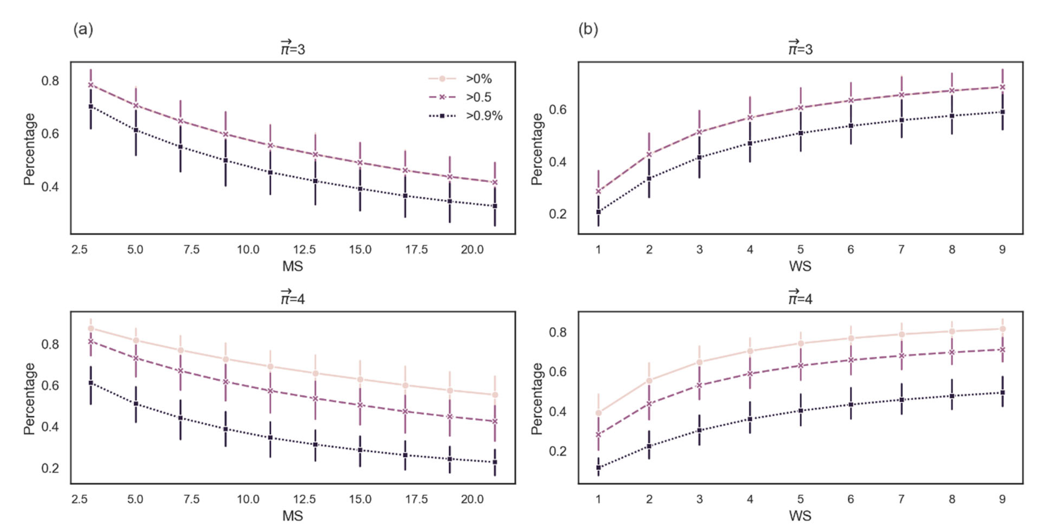
To calculate of a given path, we added a free parameter P%, which denotes the minimum percentage of consecutive words represented by a distance in the path. Here we describe the relationship between the parameters MS and WS of the distance function and the percentage of paths that receive a value given three different thresholds of P > 0, P > 0.5, and P > 0.9. As can be seen from Figure A5, for paths of length 3 and 4 and P > 0, when WS > 6, the average number of paths that receive a value is greater than 70%. However, in all cases when P > 0.5 or P > 0.9, the average number of paths that receive a value is less than 70%. In addition, for P > 0, when 9 < MS < 21, the average number of paths that receive a value is between 62% to 48%. However, for P > 0.5, the range is between 60% to 42%, and for P > 0.9, the range is 44% to 27%.
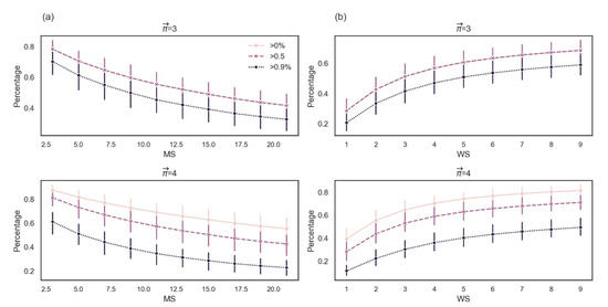
Figure A5.
Percentage of paths of length 3 or 4 that receive a value depending on the MS and WS parameters of the distance function. The rows denote different path lengths. The charts in (a) present the P% as a function of MS, and the charts in (b) present the P% as a function of WS.
Figure A5.
Percentage of paths of length 3 or 4 that receive a value depending on the MS and WS parameters of the distance function. The rows denote different path lengths. The charts in (a) present the P% as a function of MS, and the charts in (b) present the P% as a function of WS.
- 2.
- Additional Results for Section 4
Section 4 focuses on validating the measure via our assumption that expresses the extent to which the first word in the path attracts the upcoming words. Additional results regard the linear regression, which examines the relationship between attraction and , controlling for the average location and the frequency of words i and j, and all possible interactions. Here we present the following data: (1) the number of paths and edges considered in this analysis, (2) the correlation between word location and , (3) the effect of the interaction between average location and attraction on in the model that also controlled for the frequency of word i, (4) the effect of the interaction between average location and attraction on in the model that also controlled for the frequency of word j, (5) the effect of average location on , (6) the effect of frequency i on , and (7) the effect of frequency j on .
We performed all the analyses on a range of the following parameters of the distance function: MS: (3,5,7,9,11,13,15,17,19,21) and WS: (1,2,…,9).
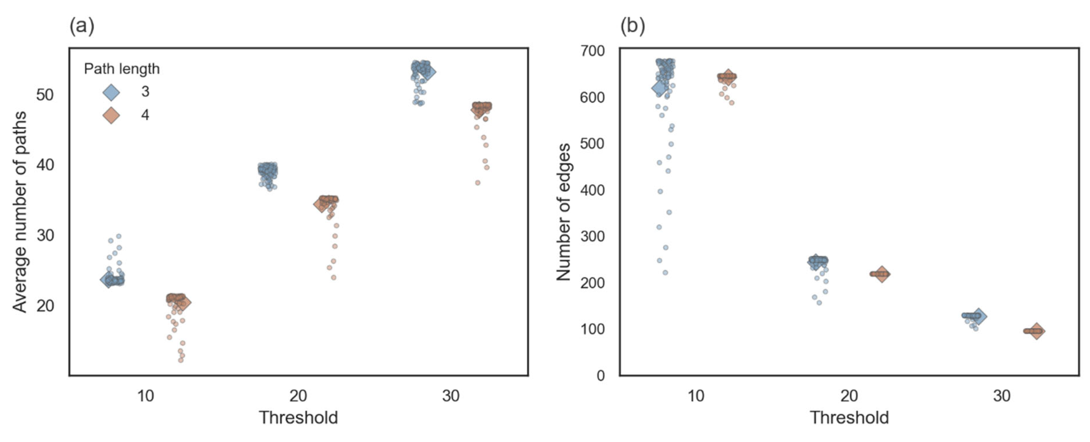
Concerning edges () that have both values and , we found on average 630.6 (SD = 16.43) edges with at least 10 paths between them, 230.8 (SD = 18.4) edges with at least 20 paths between them, and 111.1 (SD = 22.72) edges with at least 30 paths between them (Figure A6a). Concerning paths of length 3 and 4 between to , we found on average 22.08 (SD = 2.45) with least 10 paths between them, 36.67 (SD = 3.24) with at least 10 paths between them, and 50.44 (SD = 3.80) with at least 10 paths between them (Figure A6b).
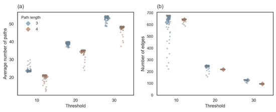
Figure A6.
(a) The average number of paths per edge (b) The average number of edges that have values and for paths of length 3 (blue) and paths of length 4 (brown). Both (a,b) reflect different combinations of the free parameters path length, WS, MS, and threshold.
Figure A6.
(a) The average number of paths per edge (b) The average number of edges that have values and for paths of length 3 (blue) and paths of length 4 (brown). Both (a,b) reflect different combinations of the free parameters path length, WS, MS, and threshold.
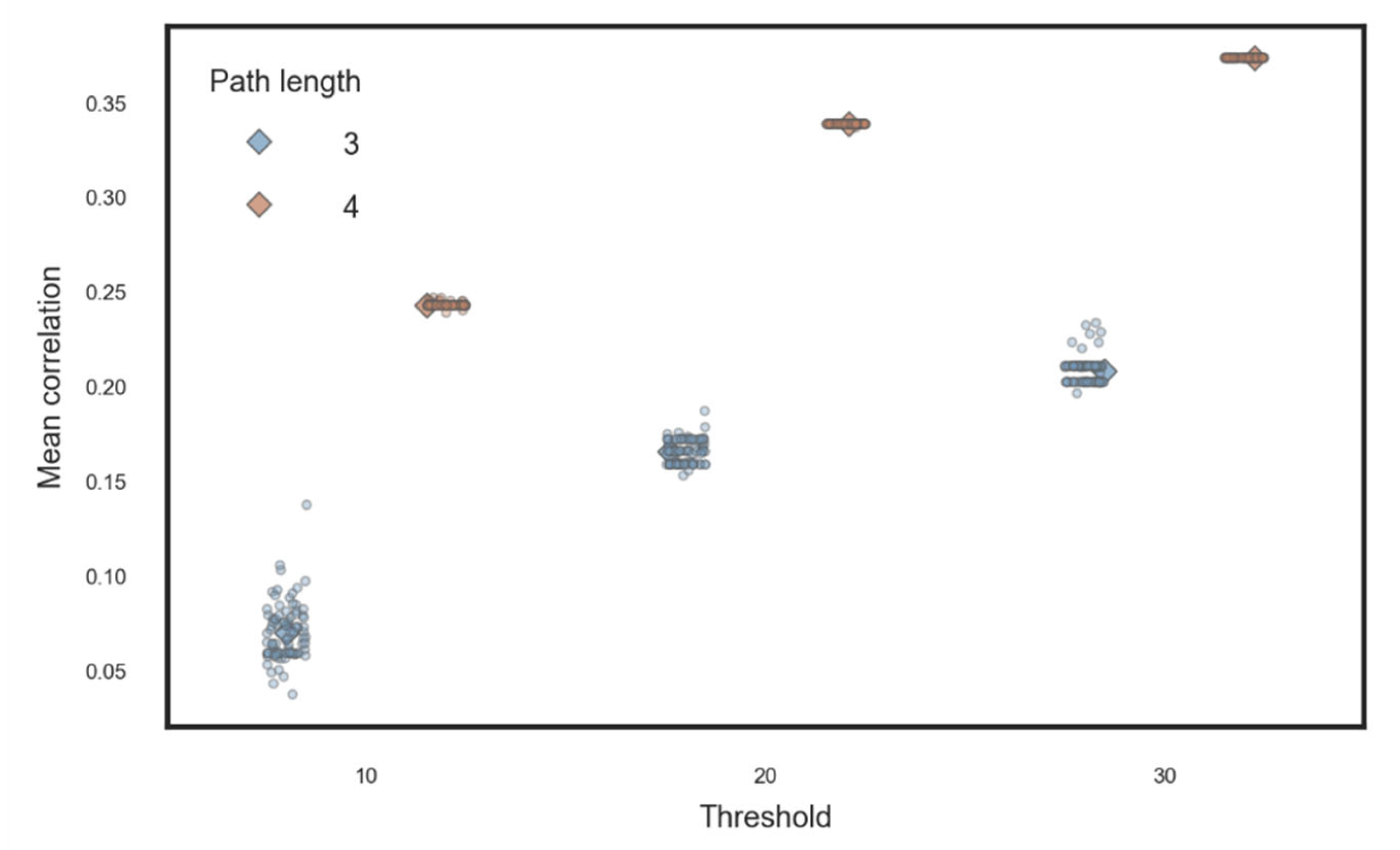
Next we controlled word location, since we found a significant correlation between the average location of a word and the transition time to the next word in our task (Figure A7).
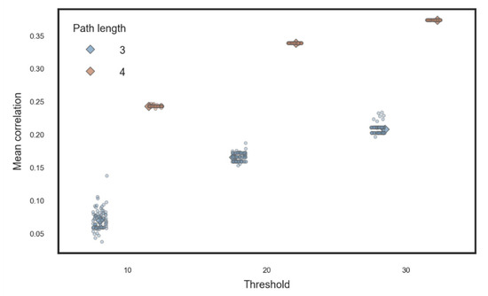
Figure A7.
The average correlation between the average location of a word and as a function of threshold and path length. The x-axis represents the threshold (10, 20, or 30). The y-axis represents the mean correlation.
Figure A7.
The average correlation between the average location of a word and as a function of threshold and path length. The x-axis represents the threshold (10, 20, or 30). The y-axis represents the mean correlation.
We now turn to the different fixed effects and the interactions between them (Figure A8, Figure A9, Figure A10, Figure A11 and Figure A12). For each heatmap, the color highlights the sign and magnitude of the beta coefficients. Blue cells indicate a negative beta, and red cells indicate a positive beta. The number of stars indicates the level of significance, the x-axis indicates the range of WS, and the y-axis indicates the range of MS. Each heatmap presents a different combination of the free parameters path length (3 or 4) and threshold (10, 20, or 30).
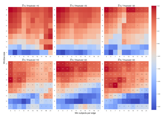
Figure A8.
The beta coefficient of the average location on in the first model, which controls for log-frequency and location of the word i.
Figure A8.
The beta coefficient of the average location on in the first model, which controls for log-frequency and location of the word i.
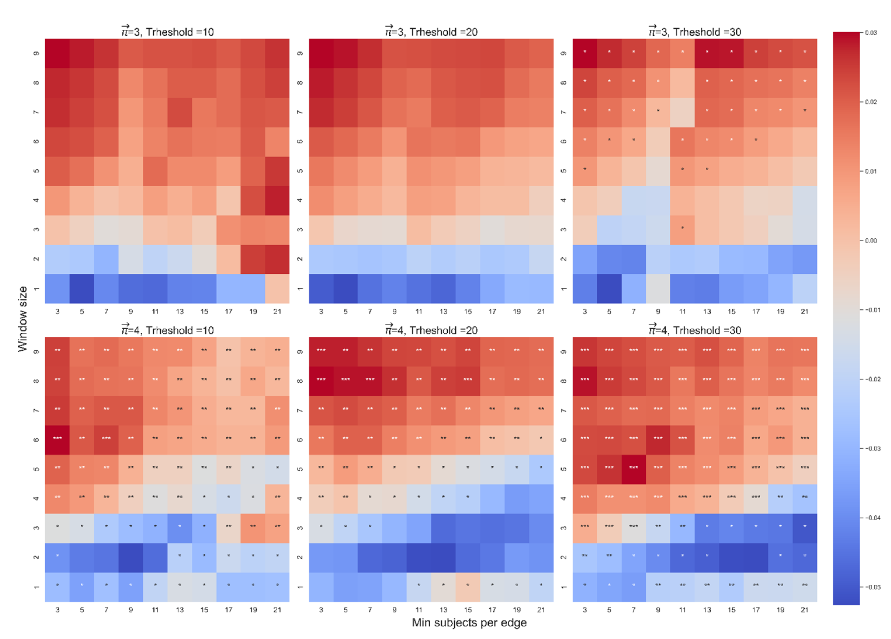

Figure A9.
The beta coefficient of the log-frequency of word i on in the first model, which controls for log-frequency and location of the word i.
Figure A9.
The beta coefficient of the log-frequency of word i on in the first model, which controls for log-frequency and location of the word i.
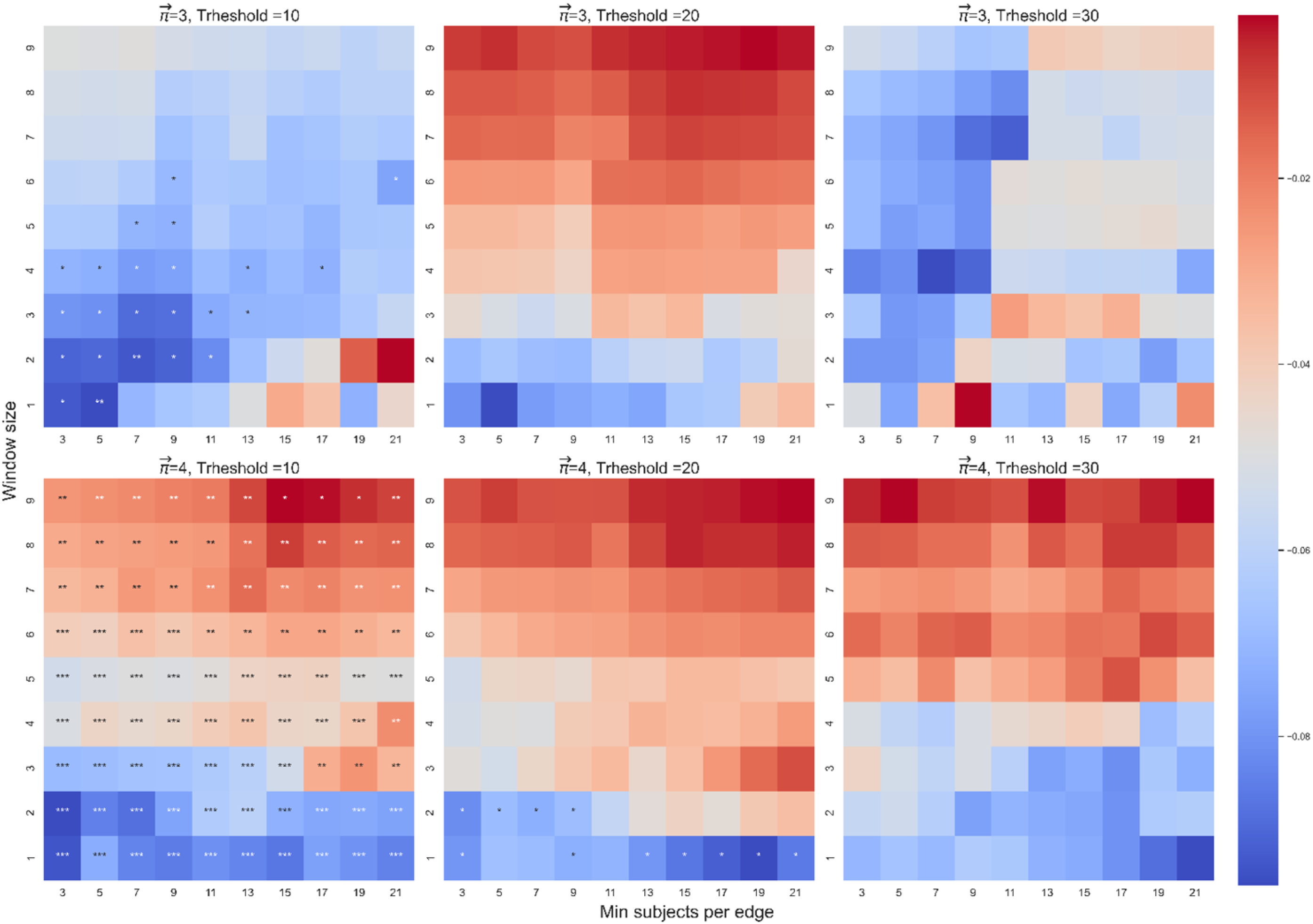
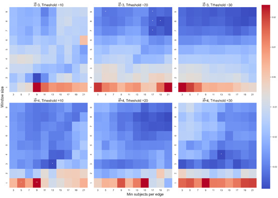
Figure A10.
The beta coefficient of the interaction between and average location on in the first and second model, which controls for log-frequency and location of word i and word j.
Figure A10.
The beta coefficient of the interaction between and average location on in the first and second model, which controls for log-frequency and location of word i and word j.

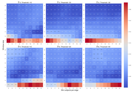
Figure A11.
The beta coefficient between and in the second model, which controls for log-frequency and location of the word j.
Figure A11.
The beta coefficient between and in the second model, which controls for log-frequency and location of the word j.
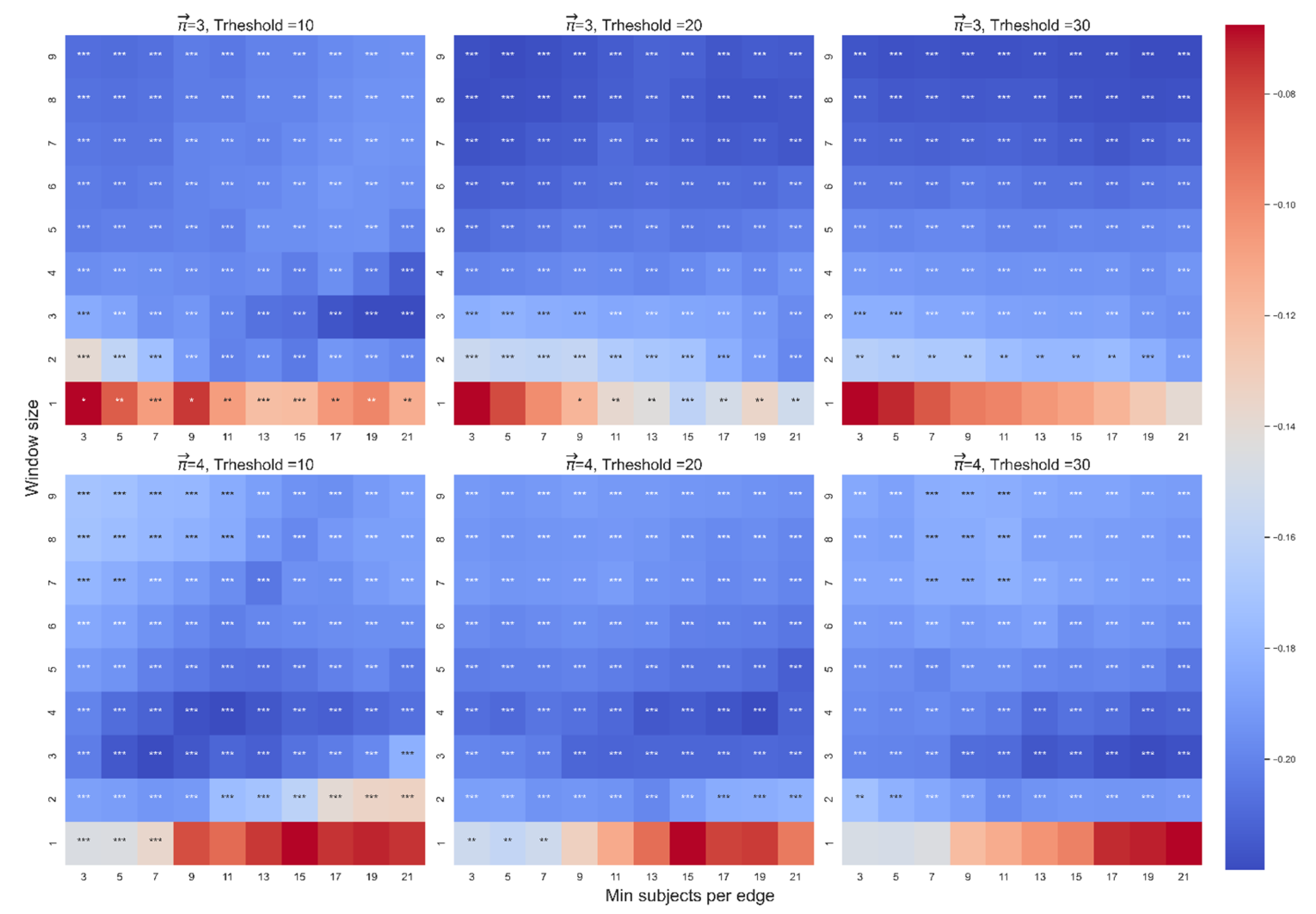

Figure A12.
The beta coefficient of the log-frequency of word j on in the second model, which controls for log-frequency and location of the word j.
Figure A12.
The beta coefficient of the log-frequency of word j on in the second model, which controls for log-frequency and location of the word j.
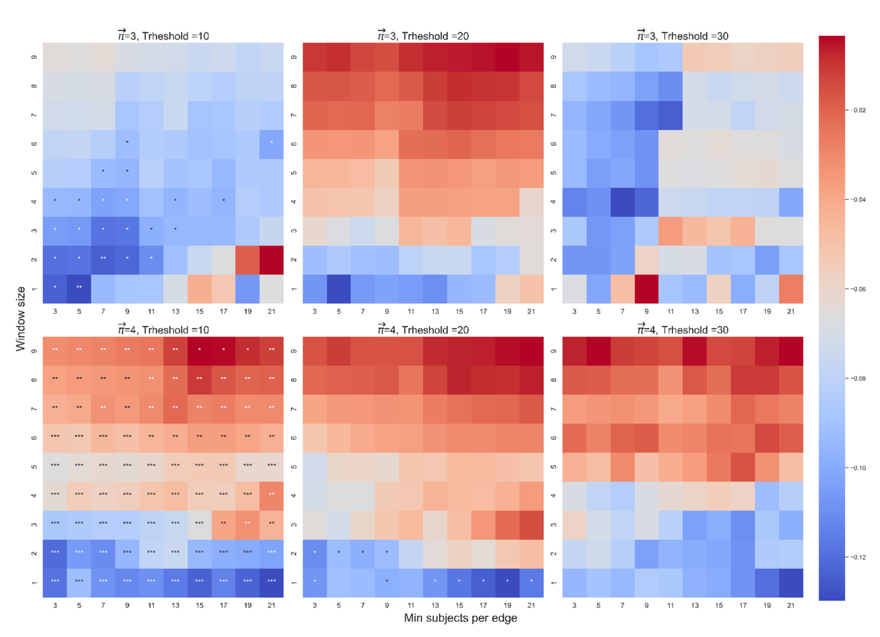
Neither model showed any robust interaction between and average location, and there was no robust significant effect of either the location or the two types of frequency on .
We evaluated four different models, each one designed to examine the effect of a single factor on dt: location, frequency of word i, frequency of word j, and attraction. The models were evaluated for a range of MS and WS values as a function of different thresholds (10, 20, 30), where a lower BIC was considered to represent the data better. The results were robust: attraction yields better results than location and both types of frequency (Figure A14).
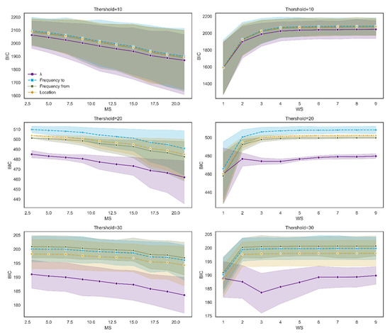
Figure A13.
The BIC score for each measure as a function of WS and MS. The first row of charts reflects threshold = 10, the second row reflects threshold = 20, and the third row reflects threshold = 30.
Figure A13.
The BIC score for each measure as a function of WS and MS. The first row of charts reflects threshold = 10, the second row reflects threshold = 20, and the third row reflects threshold = 30.

- 3.
- Additional Results for Section 5
Section 5 examines whether predicts dt-from even when we control for attraction based on the random-walker ( and for the average location of the word. Here we present additional results:
- a.
- Multicollinearity, which we tested by computing the variance inflation factor (VIF) of average location, , and (Figure A14).
- b.
- The beta coefficient between and dt-from (Figure A15). Out of 90 cases, 18 were significant for path length 3, and 21 were significant for path length 4.
- c.
- The beta coefficient for the effect of the interaction between word location on dt-from (Figure A16). Out of 90 cases, 26 were significant for path length 3, and 50 were significant for path length 4.
- d.
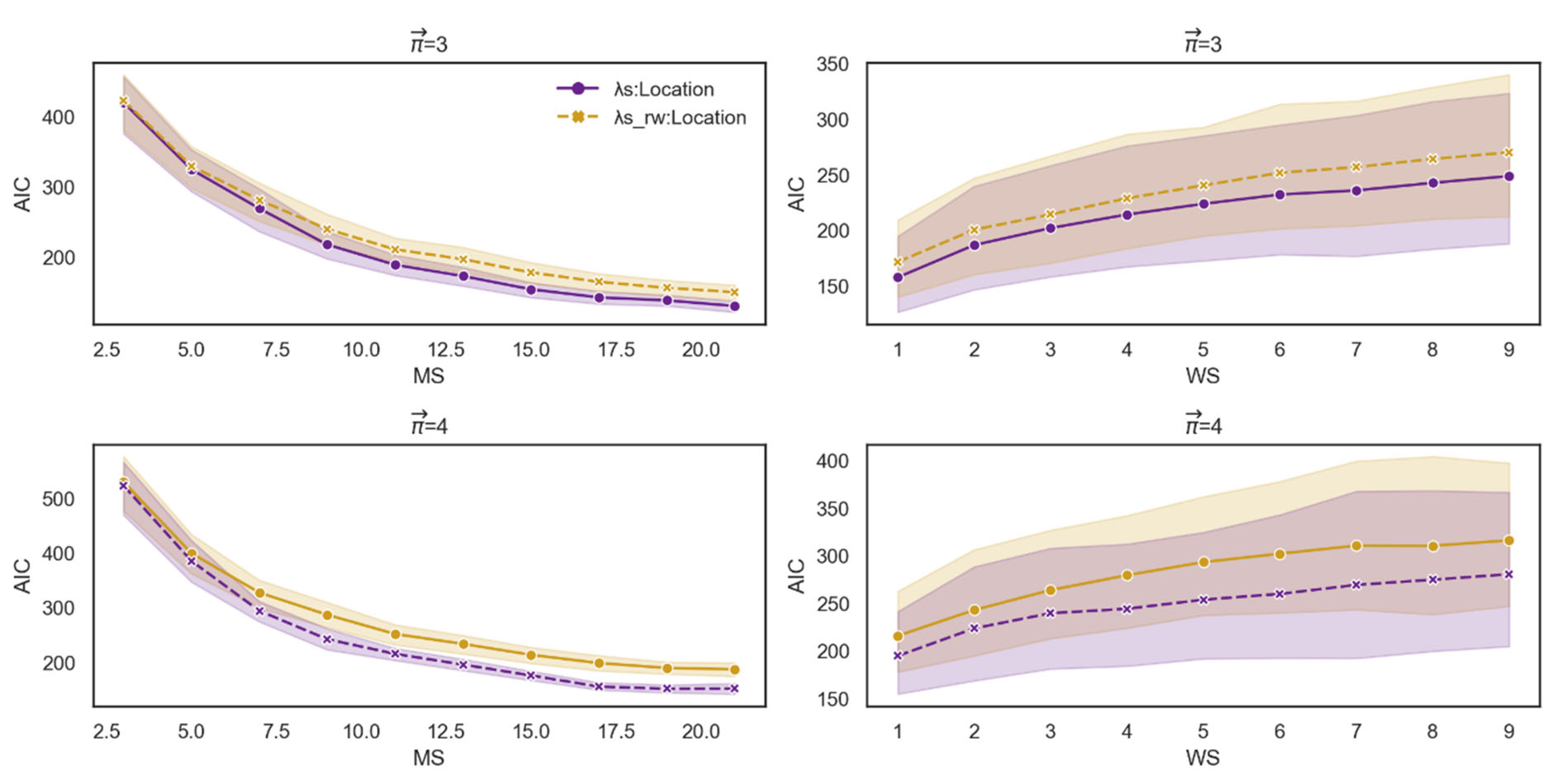
- The results of AIC, which complement the results, presented above, that we found for BIC (Figure A17).
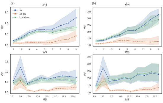
Figure A14.
The charts in column (a) present the VIF score for each measure as a function of WS and MS for path length 3. The charts in column (b) present the VIF score for each measure as a function of WS and MS for path length 4.
Figure A14.
The charts in column (a) present the VIF score for each measure as a function of WS and MS for path length 3. The charts in column (b) present the VIF score for each measure as a function of WS and MS for path length 4.
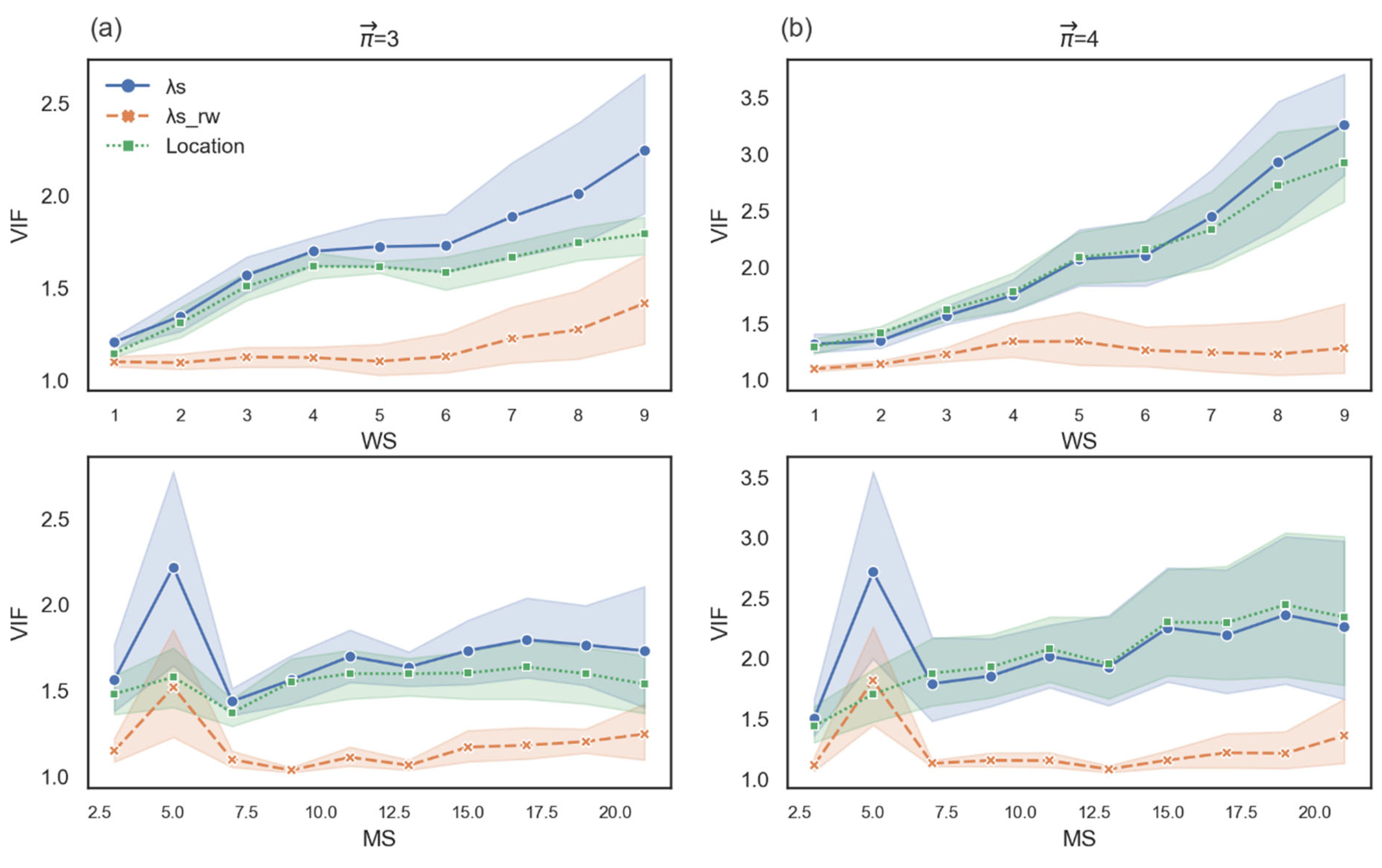
Figure A15.
Beta coefficients between and dt-from. The color highlights the sign and magnitude of the beta coefficients. Blue cells indicate a negative beta; red cells indicate a positive beta. The number of stars indicates the level of significance. The left heatmap is for paths of length 3, and the right heatmap is for paths of length 4.
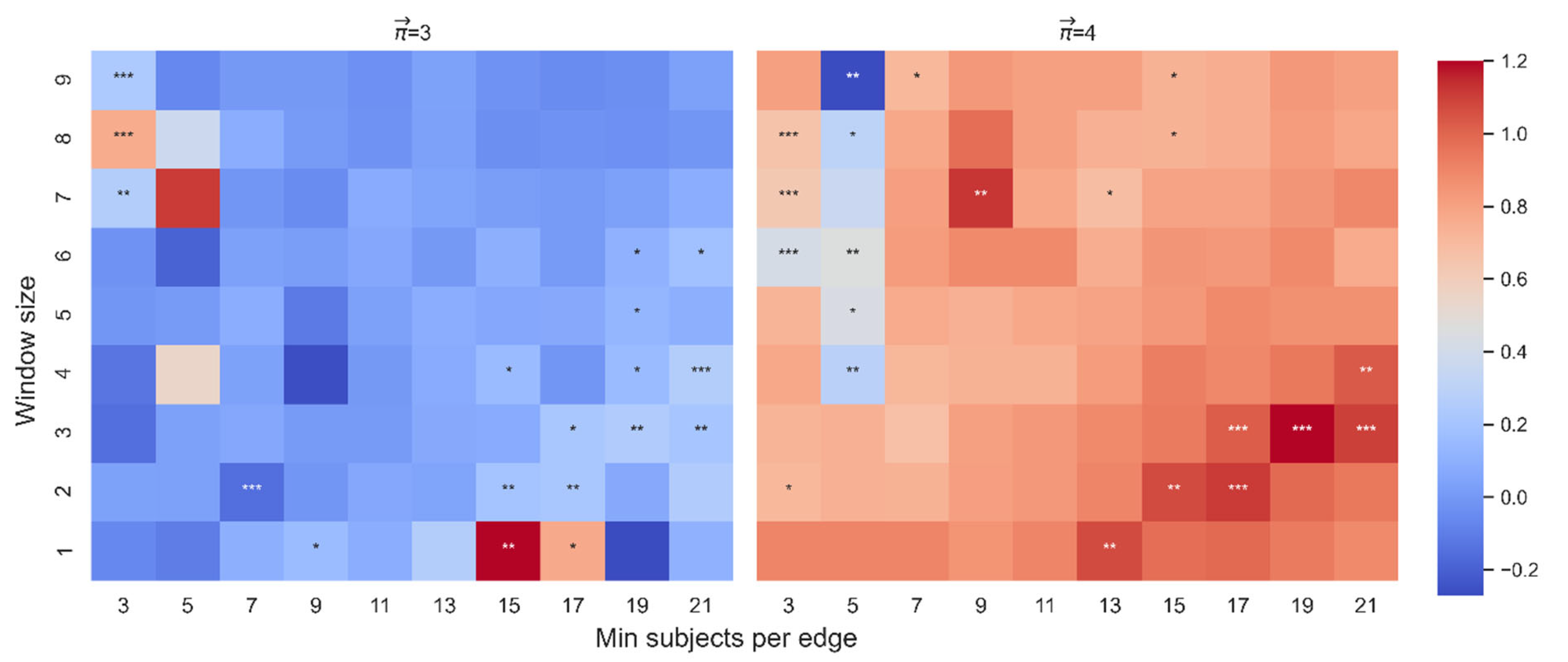
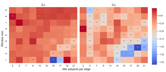
Figure A16.
The beta coefficient for the effect of the interaction between word location on dt-from. The color highlights the sign and magnitude of the beta coefficients. Blue cells indicate a negative beta; red cells indicate a positive beta. The number of stars indicates the level of significance. The left heatmap is for paths of length 3, and the right heatmap is for paths of length 4.
Figure A17.
The first row of charts presents the AIC score for each measure as a function of WS and MS for path length 3. The second row presents the AIC score for each measure as a function of WS and MS for path length.
Figure A17.
The first row of charts presents the AIC score for each measure as a function of WS and MS for path length 3. The second row presents the AIC score for each measure as a function of WS and MS for path length.
References
- Gottlieb, J.; Oudeyer, P.Y. Towards a neuroscience of active sampling and curiosity. Nat. Rev. Neurosci. 2018, 19, 758–770. [Google Scholar] [CrossRef]
- Gottlieb, J.; Cohanpour, M.; Li, Y.; Singletary, N.; Zabeh, E. Curiosity, information demand and attentional priority. Curr. Opin. Behav. Sci. 2020, 35, 83–91. [Google Scholar] [CrossRef]
- Kidd, C.; Hayden, B.Y. The psychology and neuroscience of curiosity. Neuron 2015, 88, 449–460. [Google Scholar] [CrossRef] [PubMed]
- Gershman, S.J. Uncertainty and exploration. Decision 2019, 6, 277–286. [Google Scholar] [CrossRef] [PubMed]
- Troyer, A.K.; Moscovitch, M.; Winocur, G. Clustering and switching as two components of verbal fluency:Evidence from younger and older healthy adults. Neuropsychology 1997, 11, 138–146. [Google Scholar] [CrossRef] [PubMed]
- Hills, T.T.; Jones, M.N.; Todd, P.M. Optimal foraging in semantic memory. Psychol. Rev. 2012, 119, 431–440. [Google Scholar] [CrossRef] [PubMed]
- Abbott, J.T.; Austerweil, J.L.; Griffiths, T.L. Random walks on semantic networks can resemble optimal foraging. Psychol. Rev. 2015, 122, 558–569. [Google Scholar] [CrossRef] [PubMed]
- Nachshon, Y.; Cohen, H.; Ben-Artzi, M.; Maril, A. A Model of Similarity:Metric in a Patch. PsyArXiv Preprints 2022. [Google Scholar] [CrossRef]
- Forman, R. Bochner’s method for cell complexes and combinatorial Ricci curvature. Discrete Comput. Geom. 2003, 29, 323–374. [Google Scholar] [CrossRef]
- Ollivier, Y. Ricci curvature of metric spaces. Comptes Rendus Math. 2007, 345, 643–646. [Google Scholar] [CrossRef]
- Haantjes, J. Distance geometry:curvature in abstract metric spaces. Indag. Math. 1947, 9, 302–314. [Google Scholar]
- Saucan, E.; Samal, A.; Jost, J. A simple differential geometry for complex networks. Netw. Sci. 2021, 9, S106–S133. [Google Scholar] [CrossRef]
- Saucan, E.; Appleboim, E.; Wolansky, G.; Zeevi, Y. Combinatorial Ricci curvature and Laplacians for image processing. In Proceedings of the 2nd International Congress on Image and Signal Processing, Tianjin, China, 17–19 October 2009; pp. 992–997. [Google Scholar] [CrossRef]
- Samal, A.; Pharasi, H.K.; Ramaia, S.J.; Kannan, H.; Saucan, E. Network geometry and market instability. R. Soc. Open Sci. 2021, 8, 201734. [Google Scholar] [CrossRef]
- Sandhu, R.S.; Georgiou, T.T.; Tannenbaum, A.R. Ricci curvature: An economic indicator for market fragility and systemic risk. Sci. Adv. 2016, 21–23. [Google Scholar] [CrossRef]
- Tannenbaum, A.; Sander, C.; Zhu, L.; Sandhu, R.; Kolesov, I.; Reznik, E. Graph curvature and robustness of cancer networks. arXiv 2015, arXiv:1502.04512. [Google Scholar] [CrossRef]
- Pouryahya, M.; Mathews, J.C.; Tannenbaum, A.R. Comparing three notions of discrete Ricci curvature on biological networks. Mol. Netw. 2017. [Google Scholar] [CrossRef]
- Chatterjee, T.; Albert, R.; Thapliyal, S.; Azarhooshang, N.; DasGupta, B. Detecting network anomalies using Forman–Ricci curvature and a case study for human brain networks. Sci. Rep. 2021, 11, 1–14. [Google Scholar] [CrossRef]
- Samal, A.; Sreejith, R.P.; Gu, J.; Liu, S.; Saucan, E.; Jost, J. Comparative analysis of two discretizations of Ricci curvature for complex networks. Sci. Rep. 2018, 8, 1–16. [Google Scholar] [CrossRef]
- Nachshon, Y.; Cohen, H.; Naim, P.M.; Saucan, E.; Maril, A. Ricci Curvature and the Stream of Associations. PsyArXiv Preprints 2022. [Google Scholar] [CrossRef]
- Tweedy, J.R.; Lapinski, R.H.; Schvaneveldt, R.W. Semantic-context effects on word recognition: Influence of varying the proportion of items presented in an appropriate context. Mem. Cognit. 1977, 5, 84–89. [Google Scholar] [CrossRef]
- Boersma, P.; Weenink, D. Praat: Doing Phonetics by Computer. Version 6.1.39. 2021. Available online: https://www.praat.org (accessed on 16 July 2020).
- Collins, A.M.; Loftus, E. A spreading-activation theory of semantic processing. Psychol. Rev. 1975, 82, 407–428. [Google Scholar] [CrossRef]
- Nachshon, Y.; Cohen, H.; Maril, A. Empirical Evidence For a Semantic Distance In a Patch: Investigating Symmetry and The Triangle Inequality Violations. PsyArXiv Preprints 2022. [Google Scholar] [CrossRef]
- Saucan, E. Metric curvatures and their applications I. Geom. Imaging Comput. 2015, 2, 257–334. [Google Scholar] [CrossRef]
- Caldwell-Harris, C.L. Frequency effects in reading are powerful–But is contextual diversity the more important variable? Lang Linguist. Compass 2021, 15, e12444. [Google Scholar] [CrossRef]
- Johnston, R.; Jones, K.; Manley, D. Confounding and collinearity in regression analysis:a cautionary tale and an alternative procedure, illustrated by studies of British voting behaviour. Qual. Quant. 2018, 52, 1957–1976. [Google Scholar] [CrossRef]
- Seabold, S.; Perktold, J. Statsmodels: Econometric and statistical modeling with Python. In Proceedings of the 9th Python in Science Conference, Austin, TX, USA, 28 June–3 July 2010; pp. 92–96. [Google Scholar] [CrossRef]
Publisher’s Note: MDPI stays neutral with regard to jurisdictional claims in published maps and institutional affiliations. |
© 2022 by the authors. Licensee MDPI, Basel, Switzerland. This article is an open access article distributed under the terms and conditions of the Creative Commons Attribution (CC BY) license (https://creativecommons.org/licenses/by/4.0/).

