
Investigation of the Time-Fractional Generalized Burgers–Fisher Equation via Novel Techniques


 ,
, 
Abstract
:1. Introduction
2. Preliminaries
3. Fundamental Idea of HPTM
4. Fundamental Idea of YTDM
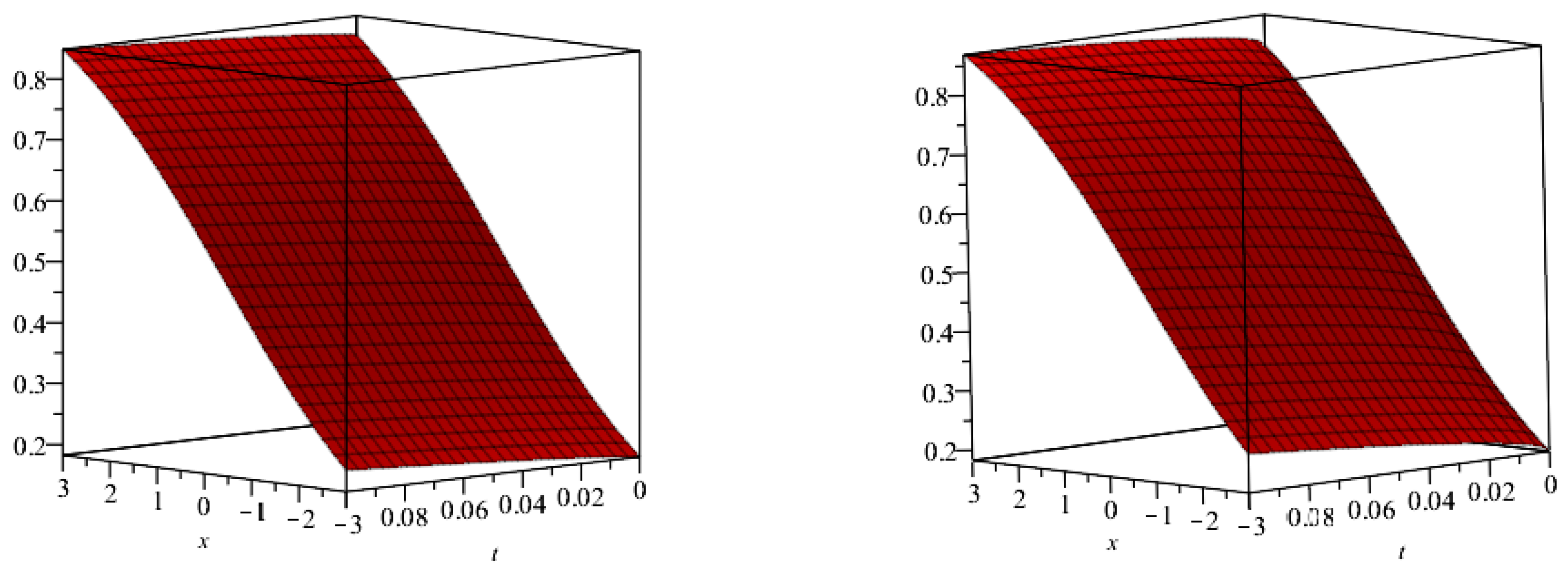
5. Numerical Examples
- By implementing
- YTDM
- On taking
- the Yang transform, we obtain
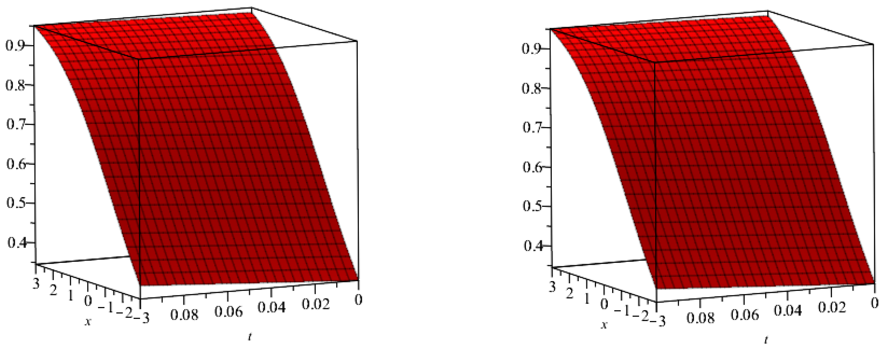
- By implementing
- YTDM
- On taking
- the Yang transform, we obtain
6. Conclusions
Author Contributions
Funding
Data Availability Statement
Acknowledgments
Conflicts of Interest
References
- Du, M.; Wang, Z.; Hu, H. Measuring memory with the order of fractional derivative. Sci. Rep. 2013, 3, 1–3. [Google Scholar] [CrossRef] [Green Version]
- Miller, K.S.; Ross, B. An introduction to Fractional Calculus and Fractional Diferential Equations; Wiley: New York, NY, USA, 1993. [Google Scholar]
- Caputo, M. Elasticita e Dissipazione; Zanichelli: Bologna, Italy, 1969. [Google Scholar]
- Liao, S.J. Homotopy analysis method: A new analytic method for nonlinear problems. Appl. Math. Mech. 1998, 19, 957–962. [Google Scholar]
- Podlubny, I. Fractional Diferential Equations; Academic Press: New York, NY, USA, 1999. [Google Scholar]
- West, B.J.; Turalskal, M.; Grigolini, P. Fractional calculus ties the microscopic and macroscopic scales of complex network dynamics. New J. Phys. 2015, 17, 1–13. [Google Scholar] [CrossRef] [Green Version]
- Tarasov, V.E. Fractional vector calculus and fractional Maxwell’s equations. Ann. Phys. 2008, 323, 2756–2778. [Google Scholar] [CrossRef] [Green Version]
- Scalar, E.; Gorenfo, R.; Mainardi, F. Fractional calculus and continuous time fnance. Phys. A 2000, 284, 376–384. [Google Scholar] [CrossRef] [Green Version]
- Kovalnogov, V.N.; Fedorov, R.V.; Chukalin, A.V.; Simos, T.E.; Tsitouras, C. Evolutionary Derivation of Runge-Kutta Pairs of Orders 5(4) SpeciallyTuned for Problems with Periodic Solutions. Mathematics 2021, 9, 2306. [Google Scholar] [CrossRef]
- Kovalnogov, V.N.; Fedorov, R.V.; Karpukhina, T.V.; Simos, T.E.; Tsitouras, C. Runge-Kutta Pairs of Orders 5(4) Trained to Best Address KeplerianType Orbits. Mathematics 2021, 9, 2400. [Google Scholar] [CrossRef]
- Wang, L.; Liu, G.; Xue, J.; Wong, K. Channel Prediction Using Ordinary Differential Equations for MIMO systems. IEEE Trans. Veh. Technol. 2022, 1–9. [Google Scholar] [CrossRef]
- El-Tantawy, S.A.; El-Sherif, L.S.; Bakry, A.M.; Alhejaili, W.; Wazwaz, A. On the analytical approximations to the nonplanar damped Kawahara equation: Cnoidal and solitary waves and their energy. Phys. Fluids 2022, 34, 113103. [Google Scholar] [CrossRef]
- El-Tantawy, S.A.; Salas, A.H.; Alyouse, H.A.; Alharthi, M.R. Novel exact and approximate solutions to the family of the forced damped Kawahara equation and modeling strong nonlinear waves in a plasma. Chin. J. Phys. 2022, 77, 2454. [Google Scholar] [CrossRef]
- El-Tantawy, S.A.; Salas, A.H.; Alyousef, H.A.; Alharthi, M.R. Novel approximations to a nonplanar nonlinear Schrödinger equation and modeling nonplanar rogue waves/breathers in a complex plasma. Chaos Solitons Fractals 2022, 163, 112612. [Google Scholar] [CrossRef]
- El-Tantawy, S.A. Nonlinear dynamics of soliton collisions in electronegative plasmas: The phase shifts of the planar KdV-and mkdV-soliton collisions. Chaos Solitons Fractals 2016, 93, 162. [Google Scholar] [CrossRef]
- Shah; El-Zahar, N.A.; Akgül, E.R.; Khan, A.; Kafle, J. Analysis of Fractional-Order Regularized Long-Wave Models via a Novel Transform. J. Funct. Spaces 2022, 2022, 2754507. [Google Scholar] [CrossRef]
- Alaoui, M.K.; Fayyaz, R.; Khan, A.; Shah, R.; Abdo, M.S. Analytical investigation of Noyes-Field model for time-fractional Belousov-Zhabotinsky reaction. Complexity 2021, 2021, 3248376. [Google Scholar] [CrossRef]
- Zidan, A.M.; Khan, A.; Shah, R.; Alaoui, M.K.; Weera, W. Evaluation of time-fractional Fisher’s equations with the help of analytical methods. AIMS Math. 2022, 7, 18746–18766. [Google Scholar] [CrossRef]
- Shah, N.A.; Hamed, Y.S.; Abualnaja, K.M.; Chung, J.D.; Shah, R.; Khan, A. A comparative analysis of fractional-order kaup-kupershmidt equation within different operators. Symmetry 2022, 14, 986. [Google Scholar] [CrossRef]
- Botmart, T.; Agarwal, R.P.; Naeem, M.; Khan, A.; Shah, R. On the solution of fractional modified Boussinesq and approximate long wave equations with non-singular kernel operators. AIMS Math. 2022, 7, 12483–12513. [Google Scholar] [CrossRef]
- Prakash, A.; Veeresha, P.; Prakasha, D.G.; Goyal, M. A new efficient technique for solving fractional coupled Navier-Stokes equations using q-homotopy analysis transform method. Pramana 2019, 93, 1–10. [Google Scholar] [CrossRef]
- Abuteen, E.; Freihat, A.; Al-Smadi, M.; Khalil, H.; Khan, R.A. Approximate series solution of nonlinear, fractional Klein-Gordon equations using fractional reduced differential transform method. arXiv 2017, arXiv:1704.06982. [Google Scholar] [CrossRef] [Green Version]
- Abuasad, S.; Hashim, I.; Abdul Karim, S.A. Modified fractional reduced differential transform method for the solution of multiterm time-fractional diffusion equations. Adv. Math. Phys. 2019, 2019, 5703916. [Google Scholar] [CrossRef] [Green Version]
- Alderremy, A.A.; Aly, S.; Fayyaz, R.; Khan, A.; Shah, R.; Wyal, N. The analysis of fractional-order nonlinear systems of third order KdV and Burgers equations via a novel transform. Complexity 2022, 2022, 4935809. [Google Scholar] [CrossRef]
- Areshi, M.; Khan, A.; Nonlaopon, K. Analytical investigation of fractional-order Newell-Whitehead-Segel equations via a novel transform. AIMS Math. 2022, 7, 6936–6958. [Google Scholar] [CrossRef]
- Feng, Z. The first-integral method to study the Burgers-Korteweg-de Vries equation. J. Phys. A Math. Gen. 2002, 35, 343. [Google Scholar] [CrossRef]
- Rezazadeh, H.; Ziabarya, B.P. Sub-equation method for the conformable fractional generalized kuramoto sivashinsky equation. Comput. Res. Prog. Appl. Sci. Eng. 2016, 2, 106–109. [Google Scholar]
- Lu, S.; Ban, Y.; Zhang, X.; Yang, B.; Liu, S.; Yin, L.; Zheng, W. Adaptive control of time delay teleoperation system with uncertain dynamics. Front. Neurorobot. 2022, 16, 928863. [Google Scholar] [CrossRef] [PubMed]
- Sunthrayuth, P.; Ullah, R.; Khan, A.; Kafle, J.; Mahariq, I.; Jarad, F. Numerical analysis of the fractional-order nonlinear system of Volterra integro-differential equations. J. Funct. Spaces 2021, 2021, 1537958. [Google Scholar] [CrossRef]
- Ban, Y.; Liu, M.; Wu, P.; Yang, B.; Liu, S.; Yin, L.; Zheng, W. Depth Estimation Method for Monocular Camera Defocus Images in Microscopic Scenes. Electronics 2022, 11, 2012. [Google Scholar] [CrossRef]
- Kbiri Alaoui, M.; Nonlaopon, K.; Zidan, A.M.; Khan, A. Analytical investigation of fractional-order cahn-hilliard and gardner equations using two novel techniques. Mathematics 2022, 10, 1643. [Google Scholar] [CrossRef]
- Xu, L.; Liu, X.; Tong, D.; Liu, Z.; Yin, L.; Zheng, W. Forecasting Urban Land Use Change Based on Cellular Automata and the PLUS Model. Land 2022, 11, 652. [Google Scholar] [CrossRef]
- Al-Sawalha, M.M.; Khan, A.; Ababneh, O.Y.; Botmart, T. Fractional view analysis of Kersten-Krasil’shchik coupled KdV-mKdV systems with non-singular kernel derivatives. AIMS Math. 2022, 7, 18334–18359. [Google Scholar] [CrossRef]
- Lu, S.; Guo, J.; Liu, S.; Yang, B.; Liu, M.; Yin, L.; Zheng, W. An Improved Algorithm of Drift Compensation for Olfactory Sensors. Appl. Sci. 2022, 12, 9529. [Google Scholar] [CrossRef]
- Dang, W.; Guo, J.; Liu, M.; Liu, S.; Yang, B.; Yin, L.; Zheng, W. A Semi-Supervised Extreme Learning Machine Algorithm Based on the New Weighted Kernel for Machine Smell. Appl. Sci. 2022, 12, 9213. [Google Scholar] [CrossRef]
- Xie, Z.; Feng, X.; Chen, X. Partial least trimmed squares regression. Chemometrics and Intelligent Laboratory Systems 2022, 221, 104486. [Google Scholar] [CrossRef]
- Tang, S.; Wu, J.; Cui, M. The nonlinear convection-reaction-diffusion equation for modelling El Niño events. Commun. Nonlinear Sci. Numer. Simul. 1996, 1, 27–31. [Google Scholar] [CrossRef]
- Fakhrusy, Q.Z.; Anggraeni, C.P.; Gunawan, P.H. Simulating water and sediment flow using swe-convection diffusion model on openmp platform. In Proceedings of the 2019 7th International Conference on Information and Communication Technology (ICoICT), Kuala Lumpur, Malaysia, 24–26 July 2019; pp. 1–6. [Google Scholar]
- Or-Roshid, H.; Rashidi, M.M. Multi-soliton fusion phenomenon of Burgers equation and fission, fusion phenomenon of Sharma-Tasso-Olver equation. J. Ocean. Eng. Sci. 2017, 2, 120–126. [Google Scholar] [CrossRef]
- Qureshi, S.; Chang, M.M.; Shaikh, A.A. Analysis of series RL and RC circuits with time-invariant source using truncated M, Atangana beta and conformable derivatives. J. Ocean. Eng. Sci. 2021, 6, 217–227. [Google Scholar] [CrossRef]
- Saad Alshehry, A.; Imran, M.; Khan, A.; Shah, R.; Weera, W. Fractional View Analysis of Kuramoto-Sivashinsky Equations with Non-Singular Kernel Operators. Symmetry 2022, 14, 1463. [Google Scholar] [CrossRef]
- Sunthrayuth, P.; Alyousef, H.A.; El-Tantawy, S.A.; Khan, A.; Wyal, N. Solving Fractional-Order Diffusion Equations in a Plasma and Fluids via a Novel Transform. J. Funct. Spaces 2022, 2022, 1899130. [Google Scholar] [CrossRef]


| (approx) | (exact) | |||||
|---|---|---|---|---|---|---|
| 0.2 | 0.525326 | 0.525308 | 0.525298 | 0.525290 | 0.525290 | |
| 0.4 | 0.550192 | 0.550167 | 0.550155 | 0.550143 | 0.550143 | |
| 0.01 | 0.6 | 0.574789 | 0.574771 | 0.574760 | 0.574748 | 0.574748 |
| 0.8 | 0.5989008 | 0.598999 | 0.598993 | 0.598987 | 0.598987 | |
| 1 | 0.622794 | 0.622778 | 0.622765 | 0.622753 | 0.622753 | |
| 0.2 | 0.525639 | 0.525623 | 0.525609 | 0.525602 | 0.525602 | |
| 0.4 | 0.550492 | 0.550471 | 0.550459 | 0.550452 | 0.550452 | |
| 0.02 | 0.6 | 0.575088 | 0.575067 | 0.575058 | 0.575053 | 0.575053 |
| 0.8 | 0.599321 | 0.599304 | 0.599294 | 0.599288 | 0.599288 | |
| 1 | 0.623089 | 0.623072 | 0.623058 | 0.623046 | 0.623046 | |
| 0.2 | 0.525952 | 0.525935 | 0.525924 | 0.525914 | 0.525914 | |
| 0.4 | 0.550798 | 0.550784 | 0.550773 | 0.550762 | 0.550762 | |
| 0.03 | 0.6 | 0.575389 | 0.575375 | 0.575364 | 0.575358 | 0.575358 |
| 0.8 | 0.599629 | 0.599608 | 0.599595 | 0.599588 | 0.599588 | |
| 1 | 0.623378 | 0.623358 | 0.623349 | 0.623340 | 0.623340 | |
| 0.2 | 0.526263 | 0.526242 | 0.526231 | 0.526225 | 0.526225 | |
| 0.4 | 0.551109 | 0.551087 | 0.551079 | 0.551071 | 0.551071 | |
| 0.04 | 0.6 | 0.575708 | 0.575688 | 0.575672 | 0.575664 | 0.575664 |
| 0.8 | 0.599907 | 0.599899 | 0.599893 | 0.599888 | 0.599888 | |
| 1 | 0.623689 | 0.623657 | 0.623642 | 0.623633 | 0.623633 | |
| 0.2 | 0.526583 | 0.526559 | 0.526545 | 0.526537 | 0.526537 | |
| 0.4 | 0.551406 | 0.551395 | 0.551386 | 0.551380 | 0.551380 | |
| 0.05 | 0.6 | 0.575997 | 0.575986 | 0.575974 | 0.575969 | 0.575969 |
| 0.8 | 0.600206 | 0.600199 | 0.600193 | 0.600188 | 0.600188 | |
| 1 | 0.623962 | 0.623941 | 0.623932 | 0.623926 | 0.623926 |
| (approx) | (exact) | |||||
|---|---|---|---|---|---|---|
| 0.2 | 0.730689 | 0.730663 | 0.730649 | 0.730641 | 0.730641 | |
| 0.4 | 0.752908 | 0.752898 | 0.752887 | 0.752874 | 0.752874 | |
| 0.01 | 0.6 | 0.774134 | 0.774115 | 0.774103 | 0.774093 | 0.774093 |
| 0.8 | 0.794267 | 0.794239 | 0.794226 | 0.794215 | 0.794215 | |
| 1 | 0.813214 | 0.813198 | 0.813183 | 0.813175 | 0.813175 | |
| 0.2 | 0.731079 | 0.731054 | 0.731033 | 0.731019 | 0.731019 | |
| 0.4 | 0.753278 | 0.753258 | 0.753245 | 0.753236 | 0.753236 | |
| 0.02 | 0.6 | 0.774489 | 0.774462 | 0.774449 | 0.774438 | 0.774438 |
| 0.8 | 0.794589 | 0.794567 | 0.794552 | 0.794540 | 0.794540 | |
| 1 | 0.813532 | 0.813505 | 0.813494 | 0.813481 | 0.813481 | |
| 0.2 | 0.731439 | 0.731418 | 0.731408 | 0.731397 | 0.731397 | |
| 0.4 | 0.753645 | 0.753624 | 0.753611 | 0.753598 | 0.753598 | |
| 0.03 | 0.6 | 0.774829 | 0.774808 | 0.774792 | 0.774782 | 0.774782 |
| 0.8 | 0.794914 | 0.794892 | 0.794879 | 0.794866 | 0.794866 | |
| 1 | 0.813834 | 0.813811 | 0.813796 | 0.813786 | 0.813786 | |
| 0.2 | 0.731827 | 0.731803 | 0.731789 | 0.731775 | 0.731775 | |
| 0.4 | 0.754015 | 0.753996 | 0.753978 | 0.753960 | 0.753960 | |
| 0.04 | 0.6 | 0.775194 | 0.775155 | 0.775139 | 0.775126 | 0.775126 |
| 0.8 | 0.795246 | 0.795215 | 0.795204 | 0.795191 | 0.795191 | |
| 1 | 0.814147 | 0.814123 | 0.814104 | 0.814092 | 0.814092 | |
| 0.2 | 0.732217 | 0.732189 | 0.732167 | 0.732153 | 0.732153 | |
| 0.4 | 0.754393 | 0.754357 | 0.754337 | 0.754321 | 0.754321 | |
| 0.05 | 0.6 | 0.775519 | 0.775499 | 0.775483 | 0.775470 | 0.775470 |
| 0.8 | 0.795587 | 0.795552 | 0.795534 | 0.795515 | 0.795515 | |
| 1 | 0.814449 | 0.814424 | 0.814407 | 0.814397 | 0.814397 |
Disclaimer/Publisher’s Note: The statements, opinions and data contained in all publications are solely those of the individual author(s) and contributor(s) and not of MDPI and/or the editor(s). MDPI and/or the editor(s) disclaim responsibility for any injury to people or property resulting from any ideas, methods, instructions or products referred to in the content. |
© 2022 by the authors. Licensee MDPI, Basel, Switzerland. This article is an open access article distributed under the terms and conditions of the Creative Commons Attribution (CC BY) license (https://creativecommons.org/licenses/by/4.0/).
Share and Cite
Alotaibi, B.M.; Shah, R.; Nonlaopon, K.; Ismaeel, S.M.E.; El-Tantawy, S.A. Investigation of the Time-Fractional Generalized Burgers–Fisher Equation via Novel Techniques. Symmetry 2023, 15, 108. https://doi.org/10.3390/sym15010108
Alotaibi BM, Shah R, Nonlaopon K, Ismaeel SME, El-Tantawy SA. Investigation of the Time-Fractional Generalized Burgers–Fisher Equation via Novel Techniques. Symmetry. 2023; 15(1):108. https://doi.org/10.3390/sym15010108
Chicago/Turabian StyleAlotaibi, Badriah M., Rasool Shah, Kamsing Nonlaopon, Sherif. M. E. Ismaeel, and Samir A. El-Tantawy. 2023. "Investigation of the Time-Fractional Generalized Burgers–Fisher Equation via Novel Techniques" Symmetry 15, no. 1: 108. https://doi.org/10.3390/sym15010108