Abstract
The complicated spectrum produced by electric and hybrid car engines is particularly sensitive to the mid-frequency range. Furthermore, sensor placement in future mobility is crucial because when the positions and orientations of sensors are altered by excessive vehicle vibration, it results in the malfunctioning of autonomous driving systems. Smart structure-based active mounting approaches have been developed to reduce engine-induced vibration. These are made to continually adjust the mounts’ dynamic properties and enhance their performances in terms of noise, vibration, and harshness (NVH) under diverse operating circumstances. It can take the place of the engine support system’s current mount technique. The performance of the source part for reducing vibration when the structure is triggered by a sinusoidal and multi-frequency signal is the main subject of this study. The overall structure, which has two active mounts based on the source-paths-receiver structure, was modeled using a lumped parameter model. In the source section, sinusoidal, amplitude modulation (AM), and frequency modulation (FM) signals were used in order to assess the effectiveness of vibration reduction in the mid-frequency band. The normalized least mean-square (NLMS) technique was utilized to assess the effectiveness of an active mounting system, and a tracking signal was employed as a control signal. The algorithm was further expanded to the multi-NLMS algorithm to monitor the complex spectral signal. This demonstrates how an active mounting system can successfully reduce vibrations when the structure is activated by many mid-frequency complex signals.
1. Introduction
Since the automotive industry switched from internal combustion engine vehicles to electric vehicles, high-efficiency engines and light-weight vehicle bodies have become increasingly important for the development of vehicles. Increasing vehicle production also increases the excitation force of the engine. However, by increasing the engine excitation force, a complex vibration will be produced, and these vibrations are transmitted to other parts, such as the gearboxes and sub-frame. Additionally, this makes an unwelcome noise that is directly tied to the driver’s surroundings. To reduce that noise, many researches were carried out, such as Sampath et al. [1] proposing a performance function for internal noise control and applying it to the three-dimensional enclosure for noise control. The noise reduction effect was more obvious with the number of actuators and positions obtained through the performance function. To control sound fields inside a three-dimensional rectangular enclosure, Moustafa et al. [2] developed a zero-spillover control scheme, and the results show that good attenuation can be obtained for the enclosure in the cases of narrow-band and broadband interferences. Vibration attenuation is accomplished by structural modifications using the conventional isolation methods, but this approach has drawbacks in terms of enhancing NVH performance in diverse operating environments.
An active engine mounting system based on a smart structure that can continuous-control dynamic characteristics has garnered a lot of interest as a way to get around these restrictions. Active vibration control has been the subject of numerous studies, including the following: PZT actuators were used for active vibration control of engines in numerous applications [3,4,5]. Through suitable adjustment and elastic vibration control product design, Schwibinger et al. [6] carried out active vibration and noise control in the powertrain. According to experimental findings, it is possible to lessen the transmission system’s noise and vibration. Jiang et al. [7] reported structure–actuator-interaction-based vibration control for a plate structure (SAI). The experimental findings show that it is possible to adjust the first and second modes and boost the plate structure’s stiffness effect. A new sort of active mount using electromechanical actuators was presented by Mansour et al. [8] to address the isolation issue with variable displacement engines (VDE). The proposed model can handle complex vibration modes, according to experiments. Through a mathematical simulation of an active engine mounting system, Zhang et al. [9] proposed a link between the input voltage and output force. The complex stiffness, magnetic field, and coil parameters impact the dynamic properties of the secondary path, according to experiments and numerical simulations.
In addition, a lot of research has concentrated on creating and enhancing the following algorithms in order to perform active vibration control: In order to locate piezoelectric actuators and sensors for active vibration control, Bruant et al. [10] used a genetic algorithm. Chhabra et al. [11] used a modified heuristic genetic algorithm to determine where piezoelectric patches should be placed on a square board. The simulation results demonstrate the effectiveness of the vibration reduction effect when ten actuators are arranged symmetrically. By comparing the performance of an active engine mount with the H2 and H schemes—two robust control algorithms—Fakhari et al. [12] evaluated its effectiveness. The outcomes demonstrate that an effective controller and active installation can enhance engine vibration performance. A mathematical model for the semi-active MR engine and transmission mount was presented by Farjoud et al. [13]. The simulation yielded the best vibration isolation performance after modifying the control parameters. The best locations for the PZT actuator and sensor in a simply supported plate were found using GA by Bruant et al. [14]. The simulation demonstrates that GA can be used to define the ideal locations. Using the GA, Tham et al. [15] suggested a method for locating laminated composite panels with bonded, dispersed piezoelectric actuators. Additionally, a finite element model was created based on first-order shear deformation theory to perform active vibration control. To enhance the performance of the LMS method, Kim et al. [16,17,18] introduced the unique model-predictive sliding mode control (MPSMC) approach. The results of an experiment to verify the effectiveness of the vibration reduction reveal that the vibration level is reduced for cantilever beams and piezoelectric strut structures. Vibration control for coupled-path structures was carried out by Liette et al. [19] using rubber mounts and piezoelectric stack actuators. The active path input signal was quantified by taking into account the interaction between the source and active routes in order to isolate the source motion. Utilizing modeling and experiments, the vibration isolation was verified at the intended source path. However, the engine itself produces a complicated signal with more than two frequencies. It is challenging to apply the quantification method to a real engine mounting system because it can only be used on a single sinusoid. For the active control of complex multi-frequency signals, many studies were implemented. Pelinescu et al. [20] proposed a method for active control of longitudinal and flexural vibrations transmitted through cylindrical struts. This method can attenuate structure-borne noise caused by gears in the helicopter nacelle. Mahapatra et al. [21] introduced active control of multiple waves in a finite-length strut and applied it to a gearbox above a helicopter’s fuselage. The optimal sensor–actuator configuration is proposed through the analysis of the feedback control of the axial–flexural coupled wave by an active spectral element model (ASEM).
2. Problem Formulation
This article’s focus is solely on regulating source mass motion when a signal with a mid-frequency range excites the structure. For analytical purposes, a two-path active structural system with integrated active elements to lessen the source motion brought on by the excitation force is investigated. The source component in Figure 1 stands for an electric power train, and the reception component is a sub-frame. One passive and two active pathways make up the path segments. In the passive approach, only a rubber mount was utilized, whereas in the active way, both a rubber mount and a piezoelectric stack actuator were used. The following actions were taken to achieve the stated goals: (1) To verify the effectiveness of vibration reduction, the mathematical model was built using a lumped parameter model. (2) In an active mounting system, the normalized least mean-square (NLMS) algorithm was used to regulate the source motion control. (3) Amplitude modulation (AM), frequency modulation (FM), and sinusoids were employed as excitation signals to validate the vibration reduction performance in the mid-frequency band. Shaker locations were taken into account in the simulation when they were not aligned (asymmetric) with the actuator line.
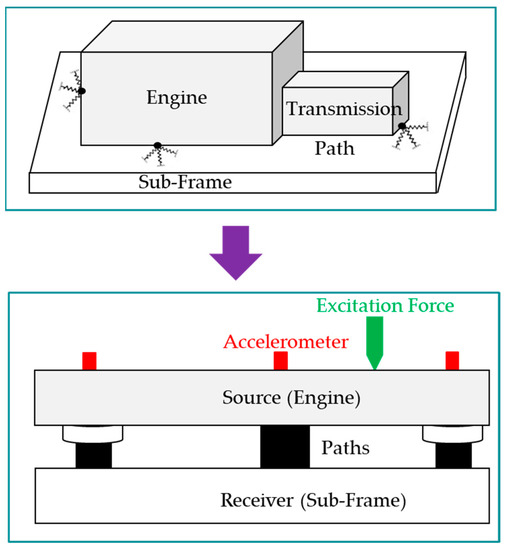
Figure 1.
Integration of active elements to lessen source movement brought on by excitation force.
The structure of this article is as follows: For a structure with two active mounting systems, Section 3 explains how to build the equation of motion using a lumped parameter model. The NLMS algorithm’s theory is explained in Section 4. The outcomes of the numerical simulation are described in Section 5. Section 6 concludes with a discussion of upcoming projects.
3. Modeling of an Active Mounting System
3.1. Lumped Parameter Approach
Based on the lumped parameter approach, the overall model with two vertically active structural paths was created, as illustrated in Figure 2. The source in this instance is analogous to an electric power train, and the receiver is analogous to a sub-frame. The path components stand in for both passive and active pathways. In the passive approach, only a rubber mount is utilized, whereas in the active way, both a rubber mount and a piezoelectric stack actuator are used.
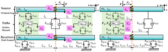
Figure 2.
Eight-DOF lumped parameter model for an asymmetric plate-like structure.
In Figure 3, and stand for the masses of the source and receiver, respectively. and represent the actuator’s mass. When the simulation was performed, the mass was measured and used. The rubber mass was also disregarded. and depict the source- and receiver-specific rotating motions in y-direction. and render the inertia in y-direction for the source and receiver, respectively. and illustrate the source and receiver-specific rotations in x-direction. and represent the inertia in x-direction for the source and receiver, respectively. and stand for the lengths to the active and rubber mount from mass center, respectively. depicts the lengths to the shaker from the mass center. , , and , render the respective stiffness and damping coefficient. , , and illustrate the control and the disturbance forces. represents the vertical motions. In this study, it is presumptive that only the z-direction of displacement and the x- and y-directions of rotational motion are taken into account. The whole model therefore comprises an 8-DOF system with four translational motions and four rotating motions. Newton’s second law can be used to describe and condense the equation of motion. The terms , , and in these equations stand in for, respectively, mass, damping, and stiffness. In addition, the terms , , and depict actuator, excitation force, and displacement, respectively. Table 1 provides a summary of the values for the specified parameters.
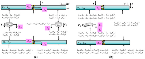
Figure 3.
Free-body diagram for (a) xz-plane and (b) yz-plane.

Table 1.
System parameters identified from a real experimental setup.
The system’s parameter values are listed in Table 1. Here, masses are given, lengths are measured, and moments of inertia are obtained from mathematical calculations. , where is the real part, is the loss factor, and . , where as the real part and as the loss factor. To determine the values of and , a chirp voltage signal applied to the actuator, and we found out the resonant frequency of the actuator through experiments. , where is the natural frequency. , where and are the half-power frequencies. The method is the same to determine the other values.
At the mass coordinates’ center, the motion equation is found. This study, however, focuses on the active mount system’s ability to reduce vibration. As a result, the equation of motion should be rewritten in terms of mounting coordinates. Figure 4 illustrates the relationship between the location of the mount and the center of mass. The locations of active path 1, active path 2, rubber mount (path 3), and the center of mass are represented in Figure 4 by the points P, Q, R, and O, respectively. Equation (6) represents the coordinate transformation after applying the internal dividing point.
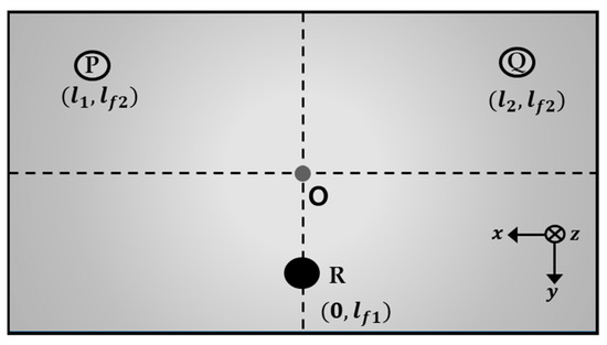
Figure 4.
Relationship between mass center and paths.
The transfer matrix is defined using the Equation (6) as follows.
Equation (7) shows the coordinate transformation, and Equation (8) expresses transformed displacement, mass, and stiffness matrices. Using Equation (8), the equation of motion can be reformulated as Equation (9). Here, superscripts stand in for the modified matrix. Equation (10) specifies the vector of amplitude displacement related to each path. Figure 5 shows different coordinate systems.
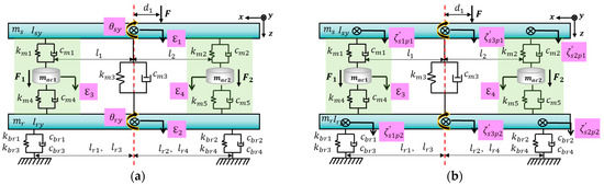
Figure 5.
Schematic of the mounting system with (a) mass coordinates and (b) mount coordinates.
3.2. State-Space Model
The simulation was carried out to confirm the impact of active paths on the source part’s vibration reduction. As a result, the state-space equation redefines the equation of motion. The block diagram and equations are represented in Figure 6 as Equations (11) and (12).
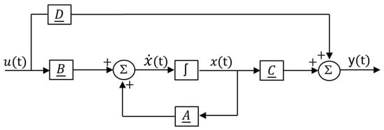
Figure 6.
Block diagram of the state-space model.
In Equations (11) and (12), , , and represent the system, input, and output matrixes, respectively, as summarized in Equations (13) and (14).
The purpose of this study was to validate the ability to reduce vibration using active mounting solutions. Each mounting path was then specified in the output , indicating that also comprises the overall path between the source and receiver, and four active and two passive paths, as summarized in Equation (15).
4. Multi-NLMS Algorithm
LMS, NLMS, and RLS adaptive filters have the ability to track or forecast the signal. As a result, adaptive algorithms are frequently used to manage the system’s noise and vibration. As a result, the NLMS algorithm was utilized to follow the source part’s active path signal in order to control it using an active mounting system. Figure 7 depicts the whole control process’s schematic. The active mounting system’s input signal is the tracked signal from the NLMS.
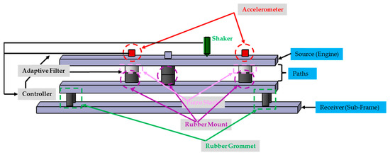
Figure 7.
Conceptual structure schematic for implementing control algorithms.
Single- and multi-frequency excitation signals are applied to the source portion using a shaker. The NLMS method controls single-frequency signals, whereas the multi-NLMS algorithm, which includes three channels, controls multi-frequency signals like AM and FM. Figure 8 displays the multi-NLMS schematic diagram.
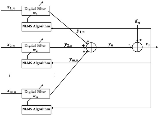
Figure 8.
Block diagram of multi-NLMS algorithm.
In Figure 8, and stand for disturbance and plant output signals, respectively. depicts the control input summing up each filter’s output, and illustrates the error signal between and . For updating the multi-NLMS algorithm with an error signal, the following filter weight updating equation is employed as Equation (16).
5. Results from Computational Analysis
Three case simulations, triggered by sinusoidal, AM, and FM signals, were carried out in order to test the vibration reduction performance through an active mounting system. The relationship between the lengths between the center of mass and the shaker and the length between the center of mass and the active mounting system determines that the shaker and active mounting system must not be on the same straight line for this series of simulations, as shown in Figure 9. A shaker was also employed in the source section to apply sinusoidal, AM, and FM signals with a mid-frequency range, with and adjusted to 30 and 60 mm.
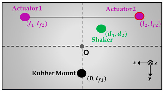
Figure 9.
Shaker and two actuators not aligned.
5.1. Sinusoids
The efficacy of vibration control is demonstrated in this section for when the active mounting system and shaker were not placed in a straight line. When the source portion is activated by a sinusoidal signal of 460 Hz, which is defined in Equation (17), the simulation was first carried out using the state-space model, which is explained in Section 3.2.
The NLMS method was also used to track the signal for an active path of the source portion. As demonstrated in Figure 10, the fast Fourier transform (FFT) was used to translate the source part’s output into the frequency domain and examine the impact of an active mounting system. Table 2 also provides an overview of peak values at the target frequency.
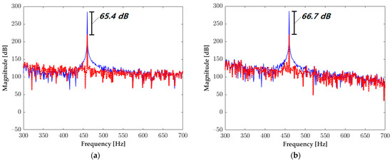
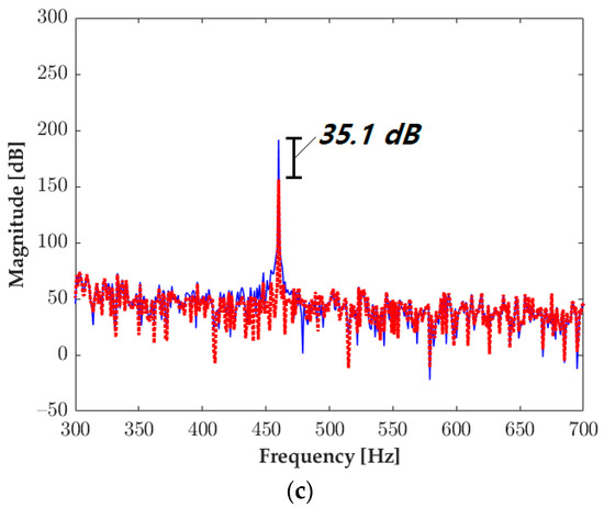
Figure 10.
Sinusoidal wave spectra at the source on (a) path 1, (b) path 2, and (c) path 3. Key: before control  , controlled with NLMS
  .
.
, controlled with NLMS .
Table 2.
Comparison of peak values at 460 Hz in the frequency domain at the source.
The blue and red lines in Figure 10 represent uncontrolled and controlled spectra, respectively. Paths 1 and 2 in Table 2 depict the active road with an active mounting mechanism, and path 3 represents the passive path, which consists of rubber grommets only. Paths 1, 2, and 3 were decreased to 65.4, 66.7, and 35.1 dB, respectively, at the desired frequency, based on the preceding results. The results of pathways 1 and 2 demonstrate significant reductions in vibration compared to path 3. This indicates that an active mounting system employing the NLMS algorithm is able to control the structure’s vibration when it is activated at mid-frequency.
5.2. Amplitude Modulated Signal
The efficiency of an active mounting system was proven in Section 5.1 when the structure was activated by a sinusoidal signal. In actuality, the electric powertrain’s vibration is typically a complex signal with a range of frequencies. Therefore, in order to properly validate an active mounting system, it is important to examine more complicated signals. As a result, the AM signal—which is specified by Equation (18)—was utilized as an excitation signal.
In addition, a three-channel multi-NLMS algorithm was used to trace the source’s active path signal. Equations (19) through (21) provide the reference signals for the three channels.
Figure 11 depicts the transformation of the output of the source component into the frequency domain, which is necessary for analyzing the influence of an active mounting system. In addition, a peak value at the frequency of interest is reported in Table 3.
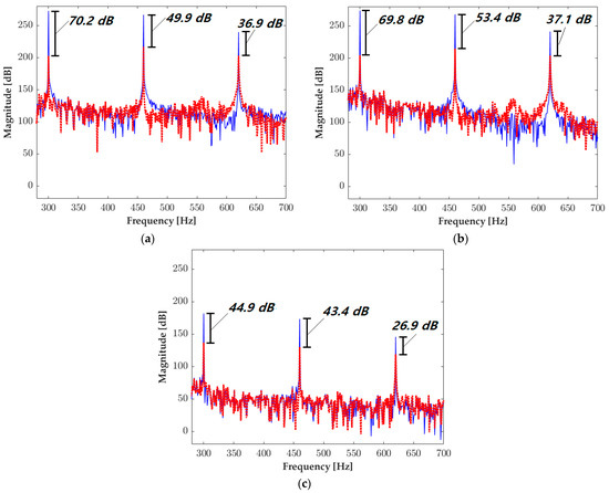
Figure 11.
Amplitude-modulated (AM) signal spectra at the source part on (a) path 1, (b) path 2, and (c) path 3. Key: before control , controlled with NLMS .
, controlled with NLMS .
Table 3.
Comparison of peak values at main frequencies (300, 460, and 620 Hz) in the frequency domain on the source part.
The blue and red lines in Figure 11 represent uncontrolled and controlled spectra, respectively. Paths 1 and 2 in Table 3 depict the active path with an active mounting mechanism, and path 3 represents the passive path, which consists of rubber grommets only. Path 1’s primary frequency was reduced by 49.9 dB, and sub-frequencies(sidebands) were reduced by 70.2 and 36.8 dB, respectively, as seen in the data above. In path 2, the primary frequency was reduced by 53,4 dB, and the sub-frequencies were reduced by 69.8 and 37.1 dB, respectively. Path 3 reveals that the principal frequency was reduced by 43.3 dB, and sub-frequencies were reduced by 44.9 and 26.9 dB, respectively.
5.3. Frequency Modulated Signal
The FM signal, which is determined by Equation (22), is utilized as an excitation signal in this section to evaluate the capability of an active mounting system in a more challenging environment because the AM signal is a relatively basic signal with three frequencies only.
For the purpose of defining the reference signal for the multi-NLMS algorithm, the system’s signal has been analyzed when the structure is excited by an FM signal. Through this study, the primary frequency that exerts the most influence on the structure was identified, which are three main frequencies. Equations (23)–(25) define the reference signal for each active path.
Figure 12 depicts the transformation of the output of the source component into the frequency domain, which is necessary for analyzing the influence of an active mounting system. Table 4 summarizes a peak value at the frequency of interest.
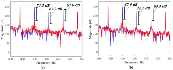
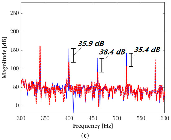
Figure 12.
Frequency modulated (FM) signal spectra at source part on (a) path 1, (b) path 2, and (c) path 3. Key: before control , controlled with NLMS .
, controlled with NLMS .
Table 4.
Comparison of peak values at main frequencies (400, 460, and 520 Hz) in the frequency domain on the source part.
The blue and red lines in Figure 12 represent uncontrolled and controlled spectra, respectively. Paths 1 and 2 in Table 4 depict the active path with an active mounting mechanism, and path 3 represents the passive path, which consists of rubber grommets only. Path 1 demonstrates that the primary frequency was reduced by 63.3 dB, and sub-frequencies were reduced by 71.2 and 61.0 dB, respectively. Path 2 further demonstrates that the primary frequency was reduced by 72.2 dB, and sub-frequencies were reduced by 67.6 and 63.3 dB, respectively. Path 3 demonstrates that the principal frequency was reduced by 38.4 dB, and sub-frequencies were reduced by 35.9 and 35.4 dB, respectively. Simulation findings of AM and FM signals indicate that when multi-NLMS is implemented in an active mounting system, the reduction of vibration is highly effective.
6. Conclusions
This work focuses on the control of source motion by means of active mounting systems comprising a piezoelectric actuator and a rubber grommet when a single or multi-frequency signal with a mid-frequency range is applied. For the purpose of validating the efficacy of active mounting systems, numerical simulations were performed to categorize the overall cases into sinusoidal, AM, and FM signals. In addition, the NLMS and multi-NLMS algorithms were used to control the source motion in active mounting systems. The following are the primary contributions of this study: (1) A sinusoidal signal was applied to the structure to validate the mid-frequency performance of an active mounting system. In addition, the vibration caused by the electric powertrain is typically a signal with several frequencies and complexity. (2) As a result, AM and FM signals were utilized in the simulation to address the severe problem. The simulation validates the performance of an active mounting system employing NLMS or multiple NLMS algorithms. In future research, a feasibility experiment should be conducted to confirm the vibration reduction’s effectiveness. In addition, for successful control, the optimal location of the active mounting system must be provided.
Author Contributions
Conceptualization, B.K.; methodology, D.H.; software, Y.Q.; writing—original draft preparation, Y.Q.; writing—review and editing, D.H. and B.K. All authors have read and agreed to the published version of the manuscript.
Funding
This work was supported by Basic Science Research Program through the National Research Foundation of Korea (NRF) funded by the Ministry of Education (NRF-2021R1A6A1A03039493 and NRF-2022R1F1A1076089).
Data Availability Statement
Not applicable.
Conflicts of Interest
The authors declare no conflict of interest.
References
- Sampath, A.; Balachandran, B. Studies on performance functions for interior noise control. Smart Mater. Struct. 1997, 6, 315–332. [Google Scholar] [CrossRef]
- Moustafa, A.B.; Balachandran, B. Control of enclosed sound fields using zero spillover schemes. J. Sound Vib. 2006, 292, 645–660. [Google Scholar]
- Sui, L.; Xiong, X.; Shi, G. Piezoelectric Actuator Design and Application on Active Vibration Control. In Proceedings of the 2012 International Conference on Solid State Devices and Materials Science, Kyoto, Japan, 25–27 September 2012; Volume 25, pp. 1388–1396. [Google Scholar]
- Roman, K.; Sven, H.; Jonathan, M.; Timo, J. Development of Active Engine Mounts Based on Piezo Actuators. ATZ Worldw. 2014, 116, 46–51. [Google Scholar]
- Santhosh, K.D.; RaviTeja, R.M.; Jayakumar, V.; SaiVirinchy, C.; Hafeez, A.A. Studies on design and material aspects of IC engine mounts for vibration reduction. Int. J. Pure Appl. Math. 2018, 118, 355–366. [Google Scholar]
- Schwibinger, P.; Hendrick, D.; Wu, W. Reduction of vibration and noise in the powertrain of passenger cars with elastomer dampers. SAE Trans. 1991, 100, 787–795. [Google Scholar]
- Jiang, J.; Gao, W.; Wang, L.; Teng, Z.; Liu, Y. Active vibration control based on modal controller considering structure-actuator interaction. J. Mech. Sci. Technol. 2018, 32, 3515–3521. [Google Scholar] [CrossRef]
- Mansour, H.; Arzanpour, S.; Golnaraghi, M.F. Active decoupler hydraulic engine mount design with application to variable displacement engine. J. Vib. Control. 2010, 17, 1498–1508. [Google Scholar] [CrossRef]
- Heng, H.Z.; Wen, K.S. Model of the Secondary Path between the Input Voltage and the Output Force of an Active Engine Mount on the Engine Side. Math. Probl. Eng. 2020, 2020, 6084169. [Google Scholar]
- Bruant, I.; Coffignal, G.; Lene, F.; Verge, M. A methodology for determination of piezoelectric actuator and sensor location on beam structures. J. Sound Vib. 2001, 243, 861–882. [Google Scholar] [CrossRef]
- Chhabra, D.; Bhushan, G.; Chandna, P. Multilevel optimization for the placement of piezo-actuators on plate structures for active vibration control using modified heuristic genetic algorithm. In Industrial and Commercial Applications of Smart Structures Technologies; SPIE: Bellingham, WA, USA, 2014. [Google Scholar]
- Vahid, F.; Abdolreza, O. Robust control of automotive engine using active engine mount. J. Vib. Control. 2012, 19, 1024–1050. [Google Scholar]
- Farjoud, A.; Taylor, R.; Schumann, E.; Schlangen, T. Advanced semi-active engine and transmission mounts: Tools for modelling, analysis, design, and tuning. Veh. Syst. Dyn. 2014, 52, 218–243. [Google Scholar] [CrossRef]
- Bruant, I.; Gallimard, L.; Nikoukar, S. Optimal piezoelectric actuator and sensor location for active vibration control using genetic algorithm. J. Sound Vib. 2010, 329, 1615–1635. [Google Scholar] [CrossRef]
- Tran, H.Q.; Vu, V.T.; Tran, M.T. optimal placement and active vibration control of composite plates integrated piezoelectric sensor/actuator pairs. J. Sci. Technol. 2018, 56, 113–126. [Google Scholar]
- Kim, B.; Washington, N.G.; Singh, R. Control of incommensurate sinusoids using enhanced adaptive filtering algorithm based on sliding mode approach. J. Vib. Control. 2012, 19, 1265–1280. [Google Scholar] [CrossRef]
- Kim, B.; Washington, N.G.; Singh, R. Control of modulated vibration using an enhanced adaptive filtering algorithm based on model-based approach. J. Sound Vib. 2012, 331, 4101–4114. [Google Scholar] [CrossRef]
- Kim, B.; Washington, N.G.; Yoon, H.S. Active vibration suppression of a 1D piezoelectric bimorph structure using model predictive sliding mode control. Smart Mater. Struct. 2013, 11, 623–635. [Google Scholar] [CrossRef]
- Liette, J.; Dreyer, J.T.; Singh, R. Interaction between two active structural paths for source mass motion control over mid-frequency range. J. Sound Vib. 2014, 333, 2369–2385. [Google Scholar] [CrossRef]
- Pelinescu, I.; Balachandran, B. Analytical study of active control of wave transmission through cylindrical struts. Smart Mater. Struct. 2001, 10, 121–136. [Google Scholar] [CrossRef]
- Mahapatra, R.D.; Gopalakrishnan, S.; Balachandran, B. Active feedback control of multiple waves in helicopter gearbox support struts. Smart Mater. Struct. 2001, 10, 1046–1058. [Google Scholar] [CrossRef]


Disclaimer/Publisher’s Note: The statements, opinions and data contained in all publications are solely those of the individual author(s) and contributor(s) and not of MDPI and/or the editor(s). MDPI and/or the editor(s) disclaim responsibility for any injury to people or property resulting from any ideas, methods, instructions or products referred to in the content. |
© 2023 by the authors. Licensee MDPI, Basel, Switzerland. This article is an open access article distributed under the terms and conditions of the Creative Commons Attribution (CC BY) license (https://creativecommons.org/licenses/by/4.0/).