LIBGRPP: A Library for the Evaluation of Molecular Integrals of the Generalized Relativistic Pseudopotential Operator over Gaussian Functions

Abstract

Generalized relativistic pseudopotentials (GRPP) of atomic cores implying the use of different potentials for atomic electronic shells with different principal quantum numbers give rise to accurate and reliable relativistic electronic structure models of atoms, molecules, clusters, and solids. These models readily incorporate the effects of Breit electron–electron interactions and one-loop quantum electrodynamics effects. Here, we report the computational procedure for evaluating one-electron integrals of GRPP over contracted Gaussian functions. This procedure was implemented in a library of routines named LIBGRPP, which can be integrated into existing quantum chemistry software, thus enabling the application of various methods to solve the many-electron problem with GRPPs. Pilot applications to electronic transitions in the ThO and UO${}_2$ molecules using the new library and intermediate-Hamiltonian Fock space relativistic coupled cluster method are presented. Deviations of excitation energies obtained within the GRPP approach from their all-electron Dirac–Coulomb–Gaunt counterparts do not exceed 50 cm${}^{-1}$ for the 31 lowest-energy states of ThO and 110 cm${}^{-1}$ for the 79 states of UO${}_2$. The results clearly demonstrate that rather economical tiny-core GRPP models can exceed in accuracy relativistic all-electron models defined by Dirac–Coulomb and Dirac–Coulomb–Gaunt Hamiltonians.

1. Introduction

The experience of computational quantum chemistry has clearly demonstrated the great importance of accounting for relativistic effects in applied ab initio modeling, especially when considering systems containing heavy atoms [1,2,3,4]. A series of approximate relativistic Hamiltonians with increasing accuracy was proposed (for review, see [5,6,7]) and implemented in general-purpose electronic structure programs, first for the special case of atomic problems [8,9,10,11,12], and then for molecular ones [13,14,15,16,17]. The latest developments in this field include models consistently accounting for frequency-dependent Breit interactions as well as the one-loop quantum electrodynamic (QED) effects [18,19,20,21,22,23,24,25]. Despite the significant progress in hardware and algorithms, such calculations based on a four-component methodology are still very demanding. They thus can be applied only to atoms and few-atomic molecular systems. The most time- and memory-consuming step in such models is accounting for magnetic (Gaunt) or total Breit two-electron interactions, which contribute, for instance, up to several hundreds of wavenumbers to electronic excitation energies even for the systems containing six-row elements, and thus cannot be omitted [2,20,26,27,28]. Either the Dirac–Coulomb Hamiltonian or its effective two-component counterparts ([6,29] and references therein) widely used in modern relativistic molecular calculations suffer from the lack of these spin-dependent two-electron interactions.

In parallel with the evolution of “genuine” relativistic Hamiltonians, the so-called pseudopotential (PP) (or, more generally, effective core potential, ECP [30]) approach was developed [31,32,33,34,35,36,37]. Originally proposed as an approximation aimed at reducing the computational cost of conventional non-relativistic calculations by removing core electrons, the pseudopotential approach was found to be an excellent alternative to scalar-relativistic Hamiltonians [38]. Further, it was modified to treat spin-dependent interactions as well [39,40]. The amazing success of the relativistic pseudopotential (RPP) approximation was due to its relatively low computational cost and the development of general purpose codes allowing one to use RPPs in routine electronic structure calculations. Another critical factor was the appearance of publicly available sets of pre-tabulated RPPs supplied by basis sets explicitly designed for pseudopotential calculations. Among such pseudopotentials, the most widely used in molecular calculations nowadays are the energy-adjusted PPs of Dolg et al. (see [35] and references therein), shape-consistent PPs of Christiansen, Ermler, Pacios, et al. [32,41,42,43,44,45,46,47,48,49], Cundari and Stevens [50], and Hay and Wadt ([51] and references therein).

However, all these RPPs were represented by semilocal operators, implying the use of a sole effective potential for each partial wave with definite spatial (l) and total (j) electronic angular momenta without discerning shells by their principal quantum numbers. Such an approximation seems to be quite reasonable when only outermost (valence) shells of atoms are treated explicitly (large core RPPs), but it becomes questionable when leaving a relatively small number of electrons in a core simulated by RPP and treating explicitly at least subvalence electrons (small core RPPs) [33,35,52,53]. The failure of semilocal RPPs occurs when valence and subvalence shells are not well separated spatially; thus, the valence–subvalence correlation effects are especially large. A typical example of such a situation is the case of processes changing the number of f-electrons in lanthanide and actinide compounds [33,36,54]. It is thus desirable to apply different potentials to the shells with the same l and j, but different principal quantum numbers. This extension of the RPP model called the generalized (or Gatchina) relativistic pseudopotential model (GRPP); it is the most widely used form of generalized relativistic effective core potential (GRECP) developed by Mosyagin, Titov and co-workers in the series of papers [33,36,37,53,54,55,56,57,58]. The latest generation of GRPPs effectively includes the Breit interaction [26,59], the effect of the finite nuclear charge distribution [37,53] and one-loop QED contributions (vacuum polarization and electron self-energy) [28]. All these effects are considered explicitly only at the GRPP generation step and then included into an electronic structure model completely at “no charge”.

In order to access the full range of features of the GRPP model in high-level ab initio calculations, one has to implement integrals of the GRPP operator for basis sets of atom-centered Gaussian functions commonly used in modern electronic structure codes. At the moment, calculations involving GRPPs can be carried out only for atomic systems using the modified version [55] of the HFD program [8] and for molecular systems using the MOLGEP program [57,60]. The latter code operates with spin-orbitals rather than two-component molecular (pseudo)spinors and thus does not allow one to treat spin-orbit interaction at the SCF level. The contributions from the effective spin-orbit operator are added at the stage of correlation calculation. The loss of accuracy due to a strongly non-optimal starting approximation for wave functions becomes significant already for the sixth row elements of the periodic table; furthermore, the opportunity to freeze the innermost explicitly treated shells after the molecular SCF step is lost. Moreover, MOLGEP is restricted to Gaussian basis functions with angular momenta only up to $l=6$ (i functions), whereas $l>6$ functions are also indispensable for the quantitative treatment of angular correlations in the states of heavy atoms with open d and/or f shells [27,28]. Other RPP integrating codes used in electronic structure simulation software can work only with conventional semilocal pseudopotentials. Among the most successful and widely used integral programs of this type allowing the use of the effective spin-orbit interaction operator are ARGOS [40,61,62] and the code written by Mitin and van Wüllen [63]. Thus, it seems reasonable to design a new modern integral code allowing the use of GRPPs and possessing no limitations arising from using a legacy code base. The interface of such a library should allow relatively simple incorporation into any widely used relativistic quantum chemistry software (e.g., DIRAC [16]).

In the present article, we report the new program implementation of molecular integrals of the GRPP operator over contracted Gaussian functions. The paper is organized as follows. In Section 2.1, the basic theory of the generalized relativistic pseudopotential model is described. The following Section 2.2, Section 2.3, Section 2.4, Section 2.5 outline the computational procedure used to evaluate three-center GRPP integrals over contracted Gaussian functions (including integrals over non-local terms of a pseudopotential). Section 3 describes in detail the LIBGRPP library implementing GRPP integrals. Pilot applications of the newly developed integral library are presented in Section 4. The final section discusses further possible improvements of LIBGRPP, and the prospects of its applications and provides some conclusive remarks. Appendices contain the discussion on problems closely related to the GRPP integral evaluation algorithm. Appendix A describes formulas for analytic differentiation of GRPP integrals, while Appendix B presents the Obara–Saika-type recurrence relations for integrals over the local part of the GRPP operator. Appendix C gives analytic expressions for one-center pseudopotential integrals.

2. Theory

2.1. Generalized Relativistic Pseudopotentials

The pseudopotential model implies the description of an explicitly treated subset of electrons with the Hamiltonian comprising the non-relativistic kinetic energy and instantaneous Coulomb electron–electron interactions,

$${\widehat{H}}^{\mathrm{RPP}}=\sum _i\left(-\frac{{\Delta }_i}{2}+\sum _{\gamma }\left(-\frac{z_{\gamma }^{\mathrm{c}}}{r_{\gamma i}}+{\widehat{U}}_{\gamma }\left(i\right)\right)\right)+\sum _{i>k}\frac{1}{r_{ik}}.$$

(1)

Here, $\gamma$ and $i,k$ run over the indices of atomic nuclei and electrons, respectively, $z_{\gamma }^{\mathrm{c}}$ stands for the effective core charge (nuclear charge minus the number of excluded electrons), $r_{\gamma i}$ ($r_{ik}$) is the distance between a nuclear center and an electron (between two electrons); atomic units are used throughout. It should be noted that if some of the atoms ${\gamma }_a$ can be described in the conventional all-electron nonrelativistic way (i.e., without a pseudopotential), then it is obvious that ${\widehat{U}}_{{\gamma }_a}\left(i\right)=0$ and $z_{{\gamma }_a}^{\mathrm{c}}$ is just the nuclear charge. The one-electron field-independent pseudopotential operator ${\widehat{U}}_{\gamma }\left(i\right)$ along with the long-range term $-z_{\gamma }^{\mathrm{c}}/r_{\gamma i}$ simulates the effect of nuclear charge and excluded electronic shells of the atom $\gamma$ on the remainder electrons. The operators ${\widehat{U}}_{\gamma }$ should bear all information on the effects of relativity. The Hamiltonian (1) is not well suited for taking into account core polarization and correlations between the excluded and explicitly treated electrons. Therefore, to achieve high accuracy in electronic structure modeling, the number of excluded electronic shells should be smaller than the number of core shells in the ordinary “chemical” sense (small-core RPP models); at least subvalence electrons are to be treated explicitly along with valence ones. Further development of this idea has led to the concept of tiny-core pseudopotentials implying an explicit treatment of several (more than one) subvalence atomic shells.

We restrict our attention to shape-consistent RPPs designed to fit the behavior of eigenfunctions of ${\widehat{H}}^{\mathrm{RPP}}$ (pseudo wavefunctions) outside of the inner core region to that of true two-component wavefunctions or large components of four-component wavefunctions. Note that pseudo wavefunctions within the inner core region are smooth and have no radial nodes. The conventional shape-consistent semilocal RPP model [38,39] assumes that an atomic contribution to molecular pseudopotential is described by the same functions (partial potentials) $U_{lj}\left(r\right)$ of the distance r from the center of the atomic nucleus (we shall omit the indices $\gamma$, i for brevity) for all spinors with spatial angular momentum l and total angular momentum j with respect of the center of this nucleus so that the overall atomic contribution is given by [31]

$${\widehat{U}}^{\mathrm{semi}-\mathrm{loc}}=\sum _{lj}{U}_{lj}\left(r\right)P_{lj},$$

(2)

where $P_{lj}$ projects onto the subspace of spinors with definite l and j values.

An accurate description of several electronic shells of an atom with different principal quantum numbers (at least valence and subvalence ones) simultaneously, i.e., the use of tiny-core RPPs seems to be hardly compatible with the Ansatz (2). The choice of $U_{lj}$ ensuring a perfect reproduction of the shape of valence pseudospinors with angular momenta l and j within the Hartree–Fock approximation for an isolated atom normally leads to a less satisfactory description of subvalence spinors with the same l and j values. This restricts the accuracy of semilocal small-core and tiny-core RPPs, especially for describing electronic structures of f-element atoms and compounds where valence and subvalence shells are not well-separated spatially. An efficient and general way to remove this restriction within the shape-consistent RPP framework is based on the use of different partial potentials $U_{nlj}\left(r\right)$ for different atomic shells (labeled by their principal quantum numbers n) [33,55]. The action of such a generalized RPP ${\widehat{U}}^{GRPP}$ on an atomic pseudospinor ${\tilde{\psi }}_{nljm}$ (m stands for the projection of j) centered on the same nucleus and is characterized by its angular momenta l and j and principal quantum number n should be equivalent to that of the corresponding partial potential $U_{nlj}$ optimized to reproduce exactly this pseudospinor:

$$\begin{array}{cc}& {\widehat{U}}^{GRPP}=\sum _{lj}{\widehat{U}}_{lj}{P}_{lj}\end{array}$$

(3)

$$\begin{array}{cc}& {\widehat{U}}_{lj}{\tilde{\psi }}_{nljm}=U_{nlj}\left(r\right){\tilde{\psi }}_{nljm}\end{array}$$

(4)

The problem of constructing a Hermitian operator ${\widehat{U}}_{lj}$ in terms of partial potentials $U_{nlj}$ and projectors $P_{nlj}$ onto the subspaces of pseudospinors with the same l, j, and n is non-trivial since $P_{nlj}$ and $U_{nlj}$ do not commute. Provided that atomic pseudospinors are solutions of an atomic Hartree–Fock problem with pseudopotentials, one can demonstrate that the Hermitian operator

$${\widehat{U}}_{lj}=\sum _n\left[U_{nlj}\left(r\right)P_{nlj}+P_{nlj}{U}_{nlj}\left(r\right)\right]-\frac{1}{2}\sum _{n{n}^{\prime }}{P}_{nlj}\left[U_{nlj}\left(r\right)+U_{n\prime lj}\left(r\right)\right]P_{n^{\prime }lj}$$

(5)

satisfies exactly the basic requirement (4) [33].

It is normally assumed that the partial potentials for atomic virtual pseudospinors coincide with that for valence subshells, $U_{n^{\prime }lj}=U_{n_{v}lj}$ for $n^{\prime }>n_v=n_v\left(l\right)$. Furthermore, in a strict analogy with conventional semilocal RPPs, partial semilocal components $U_{n_{v}lj}$ for large l are assumed l- and j-independent, $U_{n_{v}lj}\left(r\right)=U_L\left(r\right)$ for all $l>L$, where L at least should be greater than the maximum spatial angular momentum value for excluded inner-core shells. This stratagem allows one to replace the infinite summation in (3) by a finite sum [38,39].

The representation of GRPP in terms of projectors onto eigenfunctions of the total electronic angular momentum (j) is not convenient for molecular integral evaluation since the Gaussian basis functions routinely used in quantum chemistry calculations cannot be classified by the j quantum number. Therefore, for practical applications, this formula should be transformed into the spin-orbital form [39,56]. The GRPP operator can be represented as the sum of the scalar-relativistic potential (the first, second, and fourth terms in the right-hand side of Equation (6) below) and the effective spin-orbit interaction operator (the third and fifth terms):

$$\begin{array}{cc}\hfill {\widehat{U}}^{GRPP}=U_L\left(r\right)& +\sum _{l=0}^{L-1}\left[U_l\left(r\right)-U_L\left(r\right)\right]P_l+\sum _{l=1}^L{U}_l^{SO}\left(r\right)P_l\mathit{l}\mathit{s}\hfill \\ \hfill & +\sum _{l=0}^L\sum _{n_c}{\widehat{U}}_{n_{c}l}^{AREP}{P}_l+\sum _{l=1}^L\sum _{n_c}{\widehat{U}}_{n_{c}l}^{SO}{P}_l\mathit{l}\mathit{s},\hfill \end{array}$$

(6)

where $P_l=\sum _m|lm\rangle \langle lm|$ and ${\widehat{U}}_{n_{c}l}^{AREP}$ and ${\widehat{U}}_{n_{c}l}^{SO}$ are non-local operators defined as

$$\begin{array}{cc}\hfill {\widehat{U}}_{n_{c}l}^{AREP}& =\frac{l+1}{2l+1}{\widehat{V}}_{n_c,l,l+1/2}+\frac{l}{2l+1}{\widehat{V}}_{n_c,l,l-1/2}\hfill \end{array}$$

(7)

$$\begin{array}{cc}\hfill {\widehat{U}}_{n_{c}l}^{SO}& =\frac{2}{2l+1}\left[{\widehat{V}}_{n_c,l,l+1/2}-{\widehat{V}}_{n_c,l,l-1/2}\right]\hfill \end{array}$$

(8)

$$\begin{array}{cc}\hfill {\widehat{V}}_{n_c,l,j}& =\left[U_{n_{c}lj}\left(r\right)-U_{n_{v}lj}\left(r\right)\right]P_{n_{c}lj}+P_{n_{c}lj}\left[U_{n_{c}lj}\left(r\right)-U_{n_{v}lj}\left(r\right)\right]\hfill \\ \hfill & -\sum _{n_c^{\prime }}{P}_{n_{c}lj}\left[\frac{U_{n_{c}lj}\left(r\right)+U_{n_c^{\prime }lj}\left(r\right)}{2}-U_{n_{v}lj}\left(r\right)\right]P_{n_c^{\prime }lj},\hfill \end{array}$$

(9)

where $P_{n_{c}lj}\left(r\right)$ is a projector onto subvalence pseudospinors.

The accuracy of the GRPP model is restricted mainly by

• An approximate nature of the many-electron Hamiltonian used to evaluate atomic spinors, which in turn define the potentials $U_{nlj}\left(r\right)$. The construction of modern GRPPs is based on atomic four-component all-electron calculations with the Dirac–Coulomb–Breit Hamiltonian, employing Fermi nuclear charge distribution, and accounting for the quantum electrodynamic correction [28] by means of the Lamb shift model potential [18,64];
• The neglect of correlations between excluded and explicitly treated electrons and inner core polarization and smoothing of pseudo wavefunctions in the inner core area. The corresponding errors naturally decrease while reducing the number of excluded electronic shells (so-called tiny-core and empty-core versions of GRPPs [28,58]);
• A roughly approximate mean-field-like simulation of Breit interactions between the explicitly treated electrons by the corresponding contributions to one-electron GRPPs. In principle, this factor can limit the feasibility of core size reduction for heavy atoms.

For further use in molecular applications radial parts of GRPP components are expressed as linear combinations of radial Gaussian functions,

$$U\left(r\right)=\sum _k{d}_k{r}^{n_k-2}{e}^{-{\zeta }_k{r}^2},$$

(10)

where r stands for the distance from the point $\mathit{C}$ at which the RPP is centered, $r=|\mathit{r}-\mathit{C}|$. The GRPPs for chemical elements from hydrogen to element 123 were derived from Dirac–Fock(–Breit) atomic calculations in 1995–2022 and reported in the series of papers [26,33,36,37,53,54,55,56,57,58]. The parameters $n_k$, $d_k$ and ${\zeta }_k$ were tabulated and can be found in [65].

To make use of the GRPP model, one has to evaluate the integrals of the GRPP operator  (6) over some appropriate basis functions. Atom-centered Gaussian basis functions are the most widely used in modern molecular electronic structure theory; a detailed discussion can be found in the monograph [66]. Here, we will discuss only Cartesian basis sets; transformation to the spherical basis can be easily performed if necessary. Contracted basis function centered at point $\mathit{A}$ is constructed from normalized Cartesian primitive Gaussians with exponential parameters ${\alpha }_{Ai}$:

$${\varphi }_A\left(\mathit{r}\right)=\sum _i{c}_i{N}_i{x}_A^{n_A}{y}_A^{l_A}{z}_A^{m_A}{e}^{-{\alpha }_{Ai}{(\mathit{r}-\mathit{A})}^2},$$

(11)

where $x_A=x-A_x$ (the same for $y_A$ and $z_A$), $c_i$ stands for the contraction coefficients and the normalization constants are given by

$$N_i={\frac{2{\alpha }_{Ai}}{\pi }}^{3/4}\frac{{\left(4{\alpha }_{Ai}\right)}^{(n_A+l_A+m_A)/2}}{(2n_A-1)!!(2l_A-1)!!(2m_A-1)!!}.$$

(12)

The orbital angular momentum of such a contracted function is formally equal to $L_A=n_A+l_A+m_A$. Similarly, another Gaussian function ${\varphi }_B\left(\mathit{r}\right)$ centered at the point $\mathit{B}$ can be introduced. The pseudopotential operator is bound to some origin $\mathit{C}$, thus RPP integrals are in general three-center ones (see Figure 1).

One can formally define five types of molecular integrals, corresponding to each of the terms in the formula (6). However, only for the first three terms, special algorithms should be designed. These algorithms will be briefly discussed below in Section 2.2 (the local term), Section 2.3 (the semilocal scalar term), Section 2.4 (the semilocal spin-orbit term). Additional types of integrals arising from the last two non-local terms in (6) can be reduced to combinations of integrals of the first type and overlap integrals (see Section 2.5).

2.2. Scalar-Relativistic Part: Integrals over the Local Potential

Integrals $\langle {\varphi }_A|U_L\left(r\right)|{\varphi }_B\rangle$ over the first (local) term in Equation (6) are usually referred to as type 1 integrals. The most widely used algorithm for calculation of these integrals was proposed in [61] and is based on the re-expansion of Gaussian functions ${\varphi }_A$ and ${\varphi }_B$ at the origin $\mathit{C}$ where the RPP operator is centered (see Figure 1). This approach heavily suffers from numerical instabilities for the case of large exponential parameters and large angular momenta of basis functions [67]. At the same time, such basis functions have to be used in calculations with small-core and tiny-core pseudopotentials. Thus, an alternative approach is highly desirable.

The type 1 integral can be expressed in terms of integrals over unnormalized primitive Gaussian functions:

$$\langle {\varphi }_A|U_L\left(r_C\right)|{\varphi }_B\rangle =\sum _i\sum _j\sum _k{c}_i{c}_j{N}_i{N}_j{d}_k\langle {\chi }_{Ai}|r_C^{n_k-2}{e}^{-{\zeta }_k{r}_C^2}|{\chi }_{Bj}\rangle ,$$

(13)

$$\langle {\chi }_{Ai}|r_C^{n_k-2}{e}^{-{\zeta }_k{r}_C^2}|{\chi }_{Bj}\rangle =\int x_A^{n_A}{y}_A^{l_A}{z}_A^{m_A}{e}^{-{\alpha }_{Ai}}\times r_C^{n-2}{e}^{-{\zeta }_k{r}_C^2}\times x_B^{n_B}{y}_B^{l_B}{z}_B^{m_B}{e}^{-{\alpha }_{Bj}}d\mathit{r},$$

(14)

$r_C=|\mathit{r}-\mathit{C}|$. In the rest of this section, we will discuss only integrals over primitive functions $\chi$ and thus will use for brevity the notation ${\alpha }_A$, ${\alpha }_B$, $\zeta$, n instead of ${\alpha }_{Ai}$, ${\alpha }_{Bj}$, ${\zeta }_k$, $n_k$. For the overwhelming majority of pseudopotentials used nowadays (including GRPPs) the power parameter $n=0,1,2$. Moreover, since a product of Gaussian functions is again a Gaussian function, one can try to adopt the classical recurrence McMurchie–Davidson algorithm [68] (should not be confused with the McMurchie–Davidson algorithm for pseudopotential integrals proposed in [61]) for overlap integrals (the case of $n=2$) and integrals over the $\frac{1}{r_C}$ ($n=1$) [68] and $\frac{1}{r_C^2}$ ($n=2$) [69,70] operators to calculate desired pseudopotential integrals. The corresponding recurrence relations have to be slightly modified to integrate the “exponentially scaled” analogs of these operators, $e^{-\zeta r_C^2}$, $\frac{e^{-\zeta r_C^2}}{r_C}$ and $\frac{e^{-\zeta r_C^2}}{r_C^2}$. To the authors’ best knowledge, such an approach was not reported in the literature before.

The main idea of the McMurchie–Davidson algorithm [66,68] for non-PP integrals consists in the re-expansion of Gaussian overlap distributions ${\mathsf{\Omega }}_{n_A{n}_B}^x$ on the basis of Hermite Gaussian functions ${\mathsf{\Lambda }}_t$:

$${\mathsf{\Omega }}_{n_A{n}_B}^x=x_A^{n_A}{x}_B^{n_B}{e}^{-{\alpha }_A{x}_A^2}{e}^{-{\alpha }_B{x}_B^2}=\sum _{t=0}^{n_A+n_B}{E}_t^{n_A{n}_B}{\mathsf{\Lambda }}_t,$$

(15)

$${\mathsf{\Lambda }}_t\left(x\right)={\left(\frac{\partial }{\partial P_x}\right)}^t{e}^{-p{x}_P^2},$$

(16)

where $p={\alpha }_A+{\alpha }_B$ is the total exponent and $\mathit{P}=\{P_x,P_y,P_z\}$ stands for the weighted center of two primitive Gaussians, $\mathit{P}=\frac{{\alpha }_A\mathit{A}+{\alpha }_B\mathit{B}}{p}$. The re-expansion coefficients $E_t^{n_A{n}_B}$ are obtained using upward recurrence relations [66,68] starting from the base value $E_0^{00}=K_{AB}^x$, where $K_{AB}^x$ is defined as:

$$K_{AB}^x=e^{-\mu X_{AB}^2},\mu =\frac{{\alpha }_A{\alpha }_B}{{\alpha }_A+{\alpha }_B},X_{AB}=A_x-B_x.$$

(17)

The same relations are obviously held for the y and z components of the integrand in (14). If one introduces the exponential factor $e^{-\zeta r_C^2}$ related to the third center $\mathit{C}$ then the basic expansion (15) is rewritten as:

$${\tilde{\mathsf{\Omega }}}_{n_A{n}_B}^x=x_A^{n_A}{x}_B^{n_B}{e}^{-{\alpha }_A{x}_A^2}{e}^{-\zeta x_C^2}{e}^{-{\alpha }_B{x}_B^2}=\sum _{t=0}^{n_A+n_B}{\tilde{E}}_t^{n_A{n}_B}{\mathsf{\Lambda }}_t.$$

(18)

There is a product of three Gaussian functions on the right-hand side. It can be shown that the functional form of all the McMurchie–Davidson relations remains the same, but one must replace the p, $\mathit{P}$ and $K_{AB}^x$ parameters with their counterparts for the three-center case:

$$p\to q={\alpha }_A+{\alpha }_B+\zeta ,$$

(19)

$$\mathit{P}\to \mathit{Q}=\frac{{\alpha }_A\mathit{A}+{\alpha }_B\mathit{B}+\zeta \mathit{C}}{{\alpha }_A+{\alpha }_B+\zeta },$$

(20)

$$K_{AB}^x\to K_{ABC}^x=e^{-{\mu }_{AB}{X}_{AB}^2}{e}^{-{\mu }_{BC}{X}_{BC}^2}{e}^{-{\mu }_{AC}{X}_{AC}^2},$$

(21)

where ${\mu }_{AB}=\frac{{\alpha }_A{\alpha }_B}{{\alpha }_A+{\alpha }_B}$, etc. The base of recurrence relation should be modified accordingly:

$$E_0^{00}\to {\tilde{E}}_0^{00}=K_{ABC}^x.$$

(22)

Pseudopotential integrals with $n=2$ are in fact simply three-center overlap integrals, and the working formula for them is the most compact one:

$$\langle {\chi }_A|e^{-\zeta r_C^2}|{\chi }_B\rangle ={\tilde{E}}_0^{n_A{n}_B}{\tilde{E}}_0^{l_A{l}_B}{\tilde{E}}_0^{m_A{m}_B}{\left(\frac{\pi }{q}\right)}^{3/2}.$$

(23)

The expressions for the $n=0,1$ cases are more complicated:

$$\langle {\chi }_A|\frac{e^{-\zeta r_C^2}}{r_C^n}|{\chi }_B\rangle =\sum _{tuv}{\tilde{E}}_t^{n_A{n}_B}{\tilde{E}}_u^{l_A{l}_B}{\tilde{E}}_v^{m_A{m}_B}{R}_{tuv}^0,$$

(24)

$$R_{tuv}^0=\int r_C^{n-2}{\mathsf{\Lambda }}_t\left(x\right){\mathsf{\Lambda }}_u\left(y\right){\mathsf{\Lambda }}_v\left(z\right)d\mathit{r}$$

(25)

Auxiliary integrals $R_{tuv}^0$ can also be calculated via recurrence relations depending on the value of n. For $n=1$, one actually has the expressions that are identical (except for the $P\to Q$, $p\to q$ substitution) to those for ordinary nuclear-attraction integrals [66,68]:

$$R_{t+1,uv}^N=t{R}_{t-1,uv}^{N+1}+X_{QC}{R}_{tuv}^{N+1},$$

(26)

$$R_{000}^N={(-2q)}^N·F_N\left(q{R}_{QC}^2\right),$$

(27)

where $F_n\left(x\right)$ stands for the Boys function, $F_N\left(x\right)=\underset{0}{\overset{1}{\int }}{e}^{-x{t}^2}{t}^{2N}dt$ (relations for the u and v indices are similar).

For the $n=0$ case, the recurrence relations are similar to those previously published for the inverse square potential $\frac{1}{r_C^2}$ [69,70]:

$$R_{t+1,uv}^N=t{R}_{t-1,uv}^{N+1}+X_{QC}{R}_{tuv}^{N+1}-2q(t{R}_{t-1,uv}^N+X_{QC}{R}_{tuv}^N),$$

(28)

$$R_{000}^N={\left(2q\right)}^N·G_N\left(q{R}_{QC}^2\right),$$

(29)

where the function $G_N\left(x\right)$ is defined as:

$$G_N\left(x\right)=\underset{0}{\overset{1}{\int }}{e}^{-x(1-t^2)}{t}^{2N}dt,$$

(30)

and relations for the u and v indices are similar.

Equations (14) and (23)–(29) completely define the computational algorithm used to evaluate integrals over the local part of GRPP. It is beneficial to calculate the ${\tilde{E}}_t^{n_A{n}_B}$ and $R_{tuv}^N$ entities simultaneously for all the Cartesian components $(n_A,l_A,m_A)$ and $(n_B,l_B,m_B)$ in the shell pair and store them in multidimensional arrays. Even for the quite large values of angular momenta of basis functions, the amount of memory required is moderate. It is worth noting that alternative recurrence relations (Obara–Saika-like) can be obtained (their derivation is given in Appendix B), but they are less convenient for programming since all six indices denoting powers of Cartesian components are not decoupled from each other in the upward recursion formula (A29).

Approaches to stable evaluation of the $F_N\left(x\right)$ and $G_N\left(x\right)$ special functions are well-established and their description can be found elsewhere [66,68,69,70]. Unlike the paper [70] in the actual program implementation to calculate the $G_0\left(x\right)$ values at $x>12$, we use the relation employing the Dawson function $D_{+}$:

$$G_0\left(x\right)=\frac{D_{+}\left(\sqrt{x}\right)}{\sqrt{x}}$$

(31)

instead of Padé approximants to achieve an accuracy of the order ${10}^{-15}-{10}^{-16}$. At the same time, the $G_N\left(x\right)$ values for $N>0$ are still obtained within the upward recurrence relation (which is completely stable in this range of arguments).

2.3. Scalar-Relativistic Part: Integrals with Angular Projectors

The semilocal scalar term with angular projector $P_l$ gives more complicated type 2 integrals $\langle {\varphi }_A|\Delta U_l\left(r\right)P_l|{\varphi }_B\rangle$ (here and below we use for brevity $\Delta U_l$ to denote the difference potential $U_l\left(r\right)-U_L\left(r\right)$). The scheme of evaluation of type 2 integrals employed in the present work reproduces in general the half-numerical approach presented in [71,72]. It is based on the classical algorithm of McMurchie and Davidson for PP integrals [61], but radial integrals are evaluated numerically on a grid in order to overcome the well-known problem of numerical instabilities in the analytical approach.

The general idea of the algorithm consists in the re-expansion of Gaussian functions ${\varphi }_A$ and ${\varphi }_B$ at the origin $\mathit{C}$ where the pseudopotential operator is centered (see Figure 1). Then, the integration is performed over angular and radial variables separately [61]. The re-expansion yields:

$$\begin{array}{cc}\hfill \langle {\varphi }_A|\Delta U_l\left(r\right)P_l|{\varphi }_B\rangle & =\underset{0}{\overset{\infty }{\int }}\sum _m{\langle {\varphi }_A|S_{lm}\rangle }_{\mathsf{\Omega }}·\Delta U_l\left(r\right)·\sum _{m^{\prime }}{\langle {\varphi }_B|S_{l{m}^{\prime }}\rangle }_{{\mathsf{\Omega }}^{\prime }}{r}^{2}dr=\hfill \\ \hfill & =16{\pi }^2\sum _{a=0}^{n_A}\sum _{b=0}^{l_A}\sum _{c=0}^{m_A}\sum _{d=0}^{n_B}\sum _{e=0}^{l_B}\sum _{f=0}^{m_B}\left(\begin{array}{c}{n}_A\\ a\end{array}\right)\left(\begin{array}{c}{l}_A\\ b\end{array}\right)\left(\begin{array}{c}{m}_A\\ c\end{array}\right)\left(\begin{array}{c}{n}_B\\ d\end{array}\right)\left(\begin{array}{c}{l}_B\\ e\end{array}\right)\left(\begin{array}{c}{m}_B\\ f\end{array}\right)\times \hfill \\ \hfill & \times C{A}_x^{n_A-a}C{A}_y^{l_A-b}C{A}_z^{m_A-c}C{B}_x^{n_B-d}C{B}_y^{l_B-e}C{B}_z^{m_B-f}\times \hfill \\ \hfill & \times \sum _{{\lambda }_1}^{{\lambda }_{1,\max }}\sum _{{\lambda }_2}^{{\lambda }_{2,\max }}{T}_{{\lambda }_1{\lambda }_2}^{a+b+c+d+e+f}({\varphi }_A,{\varphi }_B)·\sum _{m=-l}^{+l}{\mathsf{\Omega }}_{{\lambda }_{1}lm}^{abc}\left({\widehat{\mathit{k}}}_{\mathit{A}}\right){\mathsf{\Omega }}_{{\lambda }_{2}lm}^{def}\left({\widehat{\mathit{k}}}_{\mathit{B}}\right),\hfill \\ \hfill & {\lambda }_{1,max}=l+a+b+c,{\lambda }_{2,max}=l+d+e+f\hfill \\ \hfill & {\widehat{\mathit{k}}}_A=\frac{\mathit{CA}}{|\mathit{CA}|},{\widehat{\mathit{k}}}_B=\frac{\mathit{CB}}{|\mathit{CB}|}\hfill \end{array}$$

(32)

where $\mathit{CA}=\mathit{C}-\mathit{A}$, etc., and $M_{\lambda }\left(x\right)$ stands for the modified spherical Bessel function. ${\mathsf{\Omega }}_{\lambda lm}^{abc}$ stands for angular integrals defined via real spherical harmonics $S_{lm}$ by the equation

$${\mathsf{\Omega }}_{\lambda lm}^{abc}\left(\widehat{\mathit{k}}\right)=\sum _{\mu =-\lambda }^{\lambda }{S}_{\lambda \mu }\left(\widehat{\mathit{k}}\right)\int \frac{d{\mathsf{\Omega }}_C}{4\pi }{\widehat{x}}^a{\widehat{y}}^b{\widehat{z}}^c{S}_{\lambda \mu }\left({\mathsf{\Omega }}_C\right)S_{lm}\left({\mathsf{\Omega }}_C\right).$$

(33)

The radial integral $T_{{\lambda }_1{\lambda }_2}^N$ is given by

$$T_{{\lambda }_1{\lambda }_2}^N({\varphi }_A,{\varphi }_B)=\underset{0}{\overset{\infty }{\int }}{r}^{N+2}\Delta U_l\left(r\right)F_A^{{\lambda }_1}\left(r\right)F_B^{{\lambda }_2}\left(r\right)dr$$

(34)

where $F_A^{\lambda }\left(r\right)$ and $F_B^{\lambda }\left(r\right)$ are auxiliary functions absorbing contraction coefficients of ${\varphi }_A$ and ${\varphi }_B$, respectively:

$$F_A^{\lambda }\left(r\right)=\sum _i{c}_i{N}_i{e}^{-{\alpha }_i{|\mathit{CA}|}^2-k_{Ai}{r}^2}{M}_{\lambda }\left(k_{Ai}r\right),$$

(35)

$${\mathit{k}}_{Ai}=-2{\alpha }_{Ai}·\mathit{CA},k_{Ai}=|{\mathit{k}}_{Ai}|.$$

(36)

The evaluation of angular integrals (33) is rather straightforward, and the details of the procedure can be found elsewhere [61,72]. The key step in their evaluation is to expand real spherical harmonics involved in the basis of Cartesian unitary sphere polynomials (USPs):

$$S_{lm}\left(\widehat{\mathit{r}}\right)=\sum _{r+s+t=l}{y}_{rst}^{lm}{\widehat{x}}^r{\widehat{y}}^s{\widehat{z}}^t,\widehat{\mathit{r}}=\frac{\mathit{r}}{|\mathit{r}|}$$

(37)

and then evaluate the integrals over USPs analytically. We obtain:

$${\mathsf{\Omega }}_{\lambda lm}^{abc}\left(\widehat{\mathit{k}}\right)=\sum _{\mu =-\lambda }^{+\lambda }{S}_{\lambda \mu }\left(\widehat{\mathit{k}}\right)\times \sum _{\begin{array}{c}r+s+t=\lambda \\ u+v+w=l\end{array}}{y}_{rst}^{\lambda \mu }{y}_{uvw}^{lm}\times \int {\widehat{x}}^{a+r+u}{\widehat{y}}^{b+s+v}{\widehat{z}}^{c+t+w}d\widehat{r}.$$

(38)

Integrals over unitary sphere polynomials are given by

$$\int {\widehat{x}}^i{\widehat{y}}^j{\widehat{z}}^{k}d\widehat{r}=\left\{\begin{array}{cc}4\pi \frac{(i-1)!!(j-1)!!(k-1)!!}{(i+j+k+1)!!}\hfill & \mathrm{even}i,j,k,\hfill \\ 0\hfill & \mathrm{otherwise}.\hfill \end{array}\right.$$

(39)

Explicit expression for the $y_{rst}^{lm}$ expansion coefficients can be found in [72]. Evaluation of radial integrals (34) is the most expensive step of RPP integration. However, radial integrals do not depend on powers in Cartesian multipliers of contracted Gaussian functions (11). Thus, the set of radial integrals is the same for all functions belonging to a given shell and can be pre-tabulated as the first step of the RPP integration algorithm. Angular integrals can in principle also be pre-tabulated, but practical experience shows that a large fraction of these integrals is not actually used in contractions with radial integrals. Thus, it is more computationally beneficial to calculate them “on the fly”.

In the present work, radial integrals are evaluated numerically on a grid using the Log3 scheme of Mura et al. [73]. This radial quadrature is widely used in density functional theory for integration of exchange-correlation potentials [74] and was successfully applied for evaluation of pseudopotential integrals [71]. Within this approach, the radial integral is approximated by the finite sum

$$\underset{0}{\overset{+\infty }{\int }}f\left(r\right)r^{2}dr\approx \sum _{i=1}^{n_r}{w}_{i}f\left(r_i\right).$$

(40)

Explicit expressions for the grid points $r_i$ and weights $w_i$ can be found elsewhere [71,73]. The most notable and useful feature of the Log3 quadrature (and similar schemes like the Gauss–Chebyshev quadrature [72]) is the possibility of expanding the integration grid without recalculation of the integrand values. While expanding the grid from $n_r$ to $2n_r+1$ points to refine the integral I one has to calculate only $n_r+1$ integrand values $f\left(r_i\right)$:

$$I^{\prime }=\frac{I}{2}+\sum _{i=1,3,5,\dots }^{2n_r+1}{w}_{i}f\left(r_i\right)$$

(41)

This scheme allows one to evaluate radial integrals with controllable accuracy.

The success and stability of the numerical integration using the quadrature formula imply the stability of the evaluation of the integrand function in the whole range of $r\in (0,+\infty )$. Modified spherical Bessel functions are monotonically increasing at $r\to +\infty$, and grow very fast (see Figure 2a). This is an obstacle to the direct use of the expression in the quadrature formula. To avoid numerical instabilities it was proposed [72] to switch to the scaled modified spherical Bessel function $K_{\lambda }\left(x\right)=e^{-x}{M}_{\lambda }\left(x\right)$ with the restricted value range $[0,1]$ (see Figure 2b). Thus, the expression for the auxuliary function $F_A^{\lambda }\left(r\right)$ (and also $F_B^{\lambda }\left(r\right)$) absorbing contraction coefficients of basis functions (Equation (35)) is modified as:

$$F_A^{\lambda }\left(r\right)=\sum _i{c}_i{N}_i·e^{-{\alpha }_{Ai}{|\mathit{CA}|}^2-k_{Ai}{r}^2+k_{Ai}r}{K}_{\lambda }\left(k_{Ai}r\right).$$

(42)

One can readily show that the exponential parameter in (42) is always negative at large values of r, and thus the whole integrand function tends to zero at $r\to +\infty$.

The flowchart of the algorithm used to evaluate type 2 integrals (Equation (32)) is shown on Figure 3. The first approximation to radial integrals is obtained using the grid with $n_r=31$ points. Then, the arrays containing values of the $r^N{U}_l\left(r\right)$ and $F^{\lambda }\left(r\right)$ functions at grid points with corresponding quadrature weights $w_i$ are pre-tabulated. Radial integrals $T_{{\lambda }_1{\lambda }_2}^N$ are assembled from these arrays using the formula

$$T_{{\lambda }_1{\lambda }_2}^N\approx \sum _{i=1}^{n_r}{r}_i^N\Delta U_l\left(r_i\right)F_A^{{\lambda }_1}\left(r_i\right)F_B^{{\lambda }_2}\left(r_i\right)w_i$$

(43)

for $N\le L_A+L_B$, ${\lambda }_1\le L_A+l$, ${\lambda }_2\le L_B+l$ and packed into the three-dimensional array for further use in Equation (32). Then, the grid is expanded and the next approximation to the set of radial integrals is calculated using the relation (41).

It also seems advantageous to carry out a prescreening of radial integrals before their exact evaluation. Different screening schemes were proposed in the literature [75,76,77,78]. In the present work, we have employed the quite accurate scheme proposed by Shaw and coworkers [77].

For the fast and stable evaluation of the Bessel function values, the computational scheme from [72] was adopted. The recurrence relation for the $(n+1)$-th order derivative of the $K_{\lambda }\left(x\right)$ function is:

$$K_{\lambda }^{(n+1)}\left(x\right)=\frac{\lambda }{2\lambda +1}{K}_{\lambda -1}^{\left(n\right)}\left(x\right)+\frac{\lambda +1}{2\lambda +1}{K}_{\lambda +1}^{\left(n\right)}\left(x\right)-K_{\lambda }^{\left(n\right)}\left(x\right).$$

The implementation of the scaled modified spherical Bessel function from the GSL library [79] was used to pre-tabulate reference values of $K_{\lambda }\left(x\right)$ and its first four derivatives further used in the Taylor expansion.

2.4. Integrals over the Effective Spin-Orbit Interaction Operator

The third term in the expression (6) representing the effective spin-orbit operator is quite similar to the second one. Thus, one can expect that the evaluation of corresponding molecular integrals should be only slightly more difficult than for the semilocal scalar term. Employing the relation $\mathit{s}=\frac{1}{2}\mathit{\sigma }$, we find that one should calculate integrals, which include Cartesian components of the orbital momentum operator $\mathit{l}=\{l_x,l_y,l_z\}$:

$$\langle {\varphi }_A|U_l^{SO}\left(r\right)P_l{l}_{\eta }|{\varphi }_B\rangle ,\eta =x,y,z.$$

(44)

and then combine these integrals with the Pauli matrices to construct the final molecular Hamiltonian matrix (a comprehensive discussion can be found in [15]). Integrals (44) are sometimes referred to as the type 3 integrals [40]. Using the idempotence property $P_l^2=P_l$, the fact that $P_l$ commutes with the angular momentum operator $\mathit{l}$, and the explicit expression for $P_l$, one obtain the general relation for the integrals (44):

$$\langle {\varphi }_A|U_l^{SO}\left(r\right)P_l\mathit{l}|{\varphi }_B\rangle =\underset{0}{\overset{\infty }{\int }}\sum _m{\langle {\varphi }_A|S_{lm}\rangle }_{\mathsf{\Omega }}{U}_l^{SO}\left(r\right)\sum _{m^{\prime }}\langle S_{lm}|\mathit{l}|S_{l{m}^{\prime }}\rangle {\langle {\varphi }_B|S_{l{m}^{\prime }}\rangle }_{{\mathsf{\Omega }}^{\prime }}{r}^{2}dr.$$

(45)

Following the logic of the McMurchie–Davidson approach (see Section 2.3), one arrives at the expression generally reproducing Equation (32) for type 2 integrals except for the angular part, which is transformed in the following way:

$$\sum _{m=-l}^{+l}{\mathsf{\Omega }}_{{\lambda }_{1}lm}^{abc}\left({\widehat{\mathit{k}}}_A\right){\mathsf{\Omega }}_{{\lambda }_{2}lm}^{def}\left({\widehat{\mathit{k}}}_B\right)\Rightarrow \sum _{m=-l}^{+l}\sum _{m^{\prime }=-l}^{+l}{\mathsf{\Omega }}_{{\lambda }_{1}lm}^{abc}\left({\widehat{\mathit{k}}}_A\right)\langle S_{lm}|\mathit{l}|S_{l{m}^{\prime }}\rangle {\mathsf{\Omega }}_{{\lambda }_{2}l{m}^{\prime }}^{def}\left({\widehat{\mathit{k}}}_B\right)$$

(46)

This formula seems to be more obvious and suitable for further programming than the expression for SO integrals given in [40]. The angular momentum operator matrix elements $\langle S_{lm}|\mathit{l}|S_{l{m}^{\prime }}\rangle$ in the basis of real spherical harmonics can be readily evaluated using simple textbook formulas. In the actual implementation, we construct the $\mathit{l}$ matrices in the basis of complex spherical harmonics $Y_{lm}$ and then transform it to the basis of $S_{lm}$ using the relations [66]:

$$S_{lm}=\left\{\begin{array}{cc}\frac{i}{\sqrt{2}}\left(Y_{lm}-{(-1)}^{|m|}{Y}_{l,-m}\right)\hfill & m<0,\hfill \\ Y_{l0}\hfill & m=0,\hfill \\ \frac{1}{\sqrt{2}}\left(Y_{l,-m}+{(-1)}^m{Y}_{l,m}\right)\hfill & m>0.\hfill \end{array}\right.$$

(47)

Matrix elements $\langle S_{lm}|l_{\eta }|S_{l{m}^{\prime }}\rangle$ are purely imaginary. Therefore, the final SO integrals are purely imaginary for the x and z Cartesian components and purely real for the y Cartesian component, since in (6) the imaginary integral over the $l_y$-component is multiplied by the ${\sigma }_y$ Pauli matrix, which is imaginary.

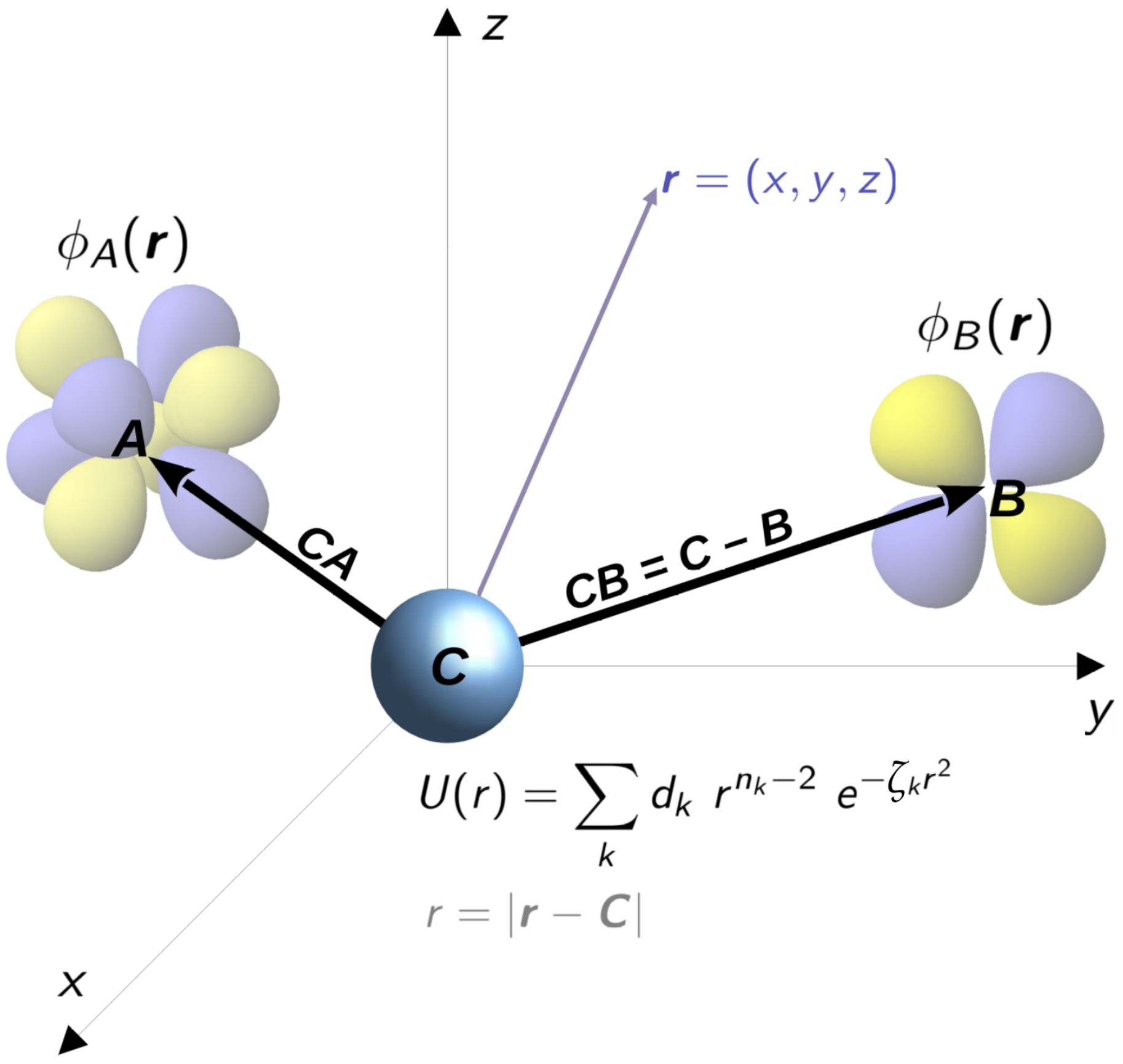
2.5. Integrals over Non-Local Terms of GRPP

The radial non-locality of the last two terms of (6) is due to the presence of projectors onto the outercore shells $P_{n_{c}lj}$. It is clear from Equations (7) and (8) that the integrals over these last terms should be assembled from the integrals over the auxiliary non-local operator ${\widehat{V}}_{n_{c}lj}$:

$$\langle {\varphi }_A|{\widehat{V}}_{n_{c}lj}|{\varphi }_B\rangle \mathrm{and}\langle {\varphi }_A|{\widehat{V}}_{n_{c}lj}{P}_l\mathit{l}|{\varphi }_B\rangle$$

(48)

Substituting the definition of ${\widehat{V}}_{n_{c}lj}$ (Equation (9)) into (48) and taking into the consideration that projectors $P_{n_{c}lj}$ do not commute with the $U_{nlj}\left(r\right)$ potentials, we formally arrive at six new types of integrals. However, they can be reduced to integrals over a local operator (type 1 integrals) discussed above in Section 2.2. The reduction is possible due to the fact that $P_{n_{c}lj}$, $P_l$, and orbital angular momentum operator $\mathit{l}$ commute with each other; at the same time, $P_l$ and $\mathit{l}$ commute with the partial (local) potential $U\left(r\right)$. Furthermore, we have an obvious relation $P_{n_{c}lj}{P}_l=P_{n_{c}lj}$. Outercore pseudospinors ${\tilde{\varphi }}_{n_{c}lj}$ used to construct the $P_{n_{c}lj}$ projectors are given simply by Gaussian expansions, therefore the evaluation of overlap integrals $\langle {\varphi }_A|{\tilde{\varphi }}_{n_{c}lj}\rangle$ and $\langle {\tilde{\varphi }}_{n_{c}lj}|{\varphi }_B\rangle$ presents no problem (in the LIBGRPP library the Obara–Saika algorithm [80] is used for fast analytical evaluation of these overlap integrals). The final expressions for the non-local terms constituting scalar-relativistic integrals in (48) are:

$$\begin{array}{cc}\hfill \langle {\varphi }_A|\left(U_{n_{c}lj}-U_{n_{v}lj}\right)P_{n_{c}lj}{P}_l|{\varphi }_B\rangle & =\sum _{m=-l}^{+l}\underset{\mathrm{type}1\mathrm{integral}}{\underbrace{\langle {\varphi }_A|U_{n_{c}lj}-U_{n_{v}lj}|{\tilde{\varphi }}_{n_{c}ljm}\rangle }}\langle {\tilde{\varphi }}_{n_{c}ljm}|{\varphi }_B\rangle ,\hfill \end{array}$$

(49)

$$\begin{array}{cc}\hfill \langle {\varphi }_A|P_{n_{c}lj}\left(U_{n_{c}lj}-U_{n_{v}lj}\right)P_l|{\varphi }_B\rangle & =\sum _{m=-l}^{+l}\langle {\varphi }_A|{\tilde{\varphi }}_{n_{c}ljm}\rangle \underset{\mathrm{type}1\mathrm{integral}}{\underbrace{\langle {\tilde{\varphi }}_{n_{c}ljm}|U_{n_{c}lj}-U_{n_{v}lj}|{\varphi }_B\rangle }},\hfill \end{array}$$

(50)

$$\begin{array}{cc}\hfill \langle {\varphi }_A|P_{n_{c}lj}\left(\frac{U_{n_{c}lj}+U_{n_c^{\prime }lj}}{2}-U_{n_{v}lj}\right)P_{n_c^{\prime }lj}{P}_l|{\varphi }_B\rangle & =\sum _{m=-l}^{+l}\langle {\varphi }_A|{\tilde{\varphi }}_{n_{c}ljm}\rangle \underset{\mathrm{purely}\mathrm{radial}\mathrm{integral}}{\underbrace{\langle {\tilde{\varphi }}_{n_{c}ljm}|\frac{U_{n_{c}lj}+U_{n_c^{\prime }lj}}{2}-U_{n_{v}lj}|{\tilde{\varphi }}_{n_c^{\prime }ljm}\rangle }}\langle {\tilde{\varphi }}_{n_c^{\prime }ljm}|{\varphi }_B\rangle ,\hfill \end{array}$$

(51)

and for the spin-orbit part:

$$\begin{array}{cc}\hfill \langle {\varphi }_A|\left(U_{n_{c}lj}-U_{n_{v}lj}\right)P_{n_{c}lj}{P}_l\mathit{l}|{\varphi }_B\rangle & =\sum _{m=-l}^{+l}\underset{\mathrm{type}1\mathrm{integral}}{\underbrace{\langle {\varphi }_A|U_{n_{c}lj}-U_{n_{v}lj}|{\tilde{\varphi }}_{n_{c}ljm}\rangle }}\sum _{m^{\prime }=-l}^{+l}\langle S_{lm}|\mathit{l}|S_{l{m}^{\prime }}\rangle \langle {\tilde{\varphi }}_{n_{c}lj{m}^{\prime }}|{\varphi }_B\rangle ,\hfill \end{array}$$

(52)

$$\begin{array}{cc}\hfill \langle {\varphi }_A|P_{n_{c}lj}\left(U_{n_{c}lj}-U_{n_{v}lj}\right)P_l\mathit{l}|{\varphi }_B\rangle & =\sum _{m=-l}^{+l}\langle {\varphi }_A|{\tilde{\varphi }}_{n_{c}ljm}\rangle \sum _{m^{\prime }=-l}^{+l}\langle S_{lm}|\mathit{l}|S_{l{m}^{\prime }}\rangle \underset{\mathrm{type}1\mathrm{integral}}{\underbrace{\langle {\tilde{\varphi }}_{n_{c}lj{m}^{\prime }}|U_{n_{c}lj}-U_{n_{v}lj}|{\varphi }_B\rangle }},\hfill \end{array}$$

(53)

$$\begin{array}{cc}\hfill \langle {\varphi }_A|P_{n_{c}lj}\left(\frac{U_{n_{c}lj}+U_{n_c^{\prime }lj}}{2}-U_{n_{v}lj}\right)P_{n_c^{\prime }lj}{P}_l\mathit{l}|{\varphi }_B\rangle & =\sum _{m=-l}^{+l}\langle {\varphi }_A|{\tilde{\varphi }}_{n_{c}ljm}\rangle \underset{\mathrm{purely}\mathrm{radial}\mathrm{integral}}{\underbrace{\langle {\tilde{\varphi }}_{n_{c}ljm}|\frac{U_{n_{c}lj}+U_{n_c^{\prime }lj}}{2}-U_{n_{v}lj}|{\tilde{\varphi }}_{n_c^{\prime }ljm}\rangle }}\times \hfill \\ \hfill & \times \sum _{m^{\prime }=-l}^{+l}\langle S_{lm}|\mathit{l}|S_{l{m}^{\prime }}\rangle \langle {\tilde{\varphi }}_{n_c^{\prime }ljm}|{\varphi }_B\rangle .\hfill \end{array}$$

(54)

The integral arising in the right-hand side of formulas (51) and (54) is purely radial:

$$\langle {\tilde{\varphi }}_{n_{c}ljm}|\frac{U_{n_{c}lj}+U_{n_c^{\prime }lj}}{2}-U_{n_{v}lj}|{\tilde{\varphi }}_{n_c^{\prime }ljm}\rangle =\underset{0}{\overset{+\infty }{\int }}\left(\frac{U_{n_{c}lj}+U_{n_c^{\prime }lj}}{2}-U_{n_{v}lj}\right)R_{n_{c}lj}\left(r\right)R_{n_c^{\prime }lj}\left(r\right)r^{2}dr,$$

(55)

where $R_{n_{c}lj}\left(r\right)$ stand for radial parts of subvalence (outercore) atomic pseudospinors ${\tilde{\varphi }}_{n_{c}ljm}$ expressed as linear combinations of Gaussians. This integral is obviously independent on m and can be taken out of the summation, leaving only the multiplication of overlap matrices in (51) or two consecutive multiplications involving overlap and angular momentum operator matrices in (54). Note that in the reference implementation of GRPP integrals (MOLGEP package) matrix elements (51) and (54), which are off-diagonal in the $n_c$ quantum number are omitted. However, they can be of the same magnitude as the diagonal elements (for example, this occurs for the uranium GRPP from [65]). Integrals (55) are evaluated analytically (see Appendix C). Gaussian expansions of radial functions $R_{n_{c}lj}\left(r\right)$ are obtained only once at the GRPP generation stage and are listed in GRPP data files published online [56,65].

Similarly to local and semilocal terms of GRPP, all integrals over non-local terms are also calculated in batches for all pairs of Cartesian Gaussians in a shell pair simultaneously. In practice, the integration of non-local terms is even faster than the integration of the “conventional” semilocal RPP operator due to the use of type 1 integrals in all working formulas. These formulas are very simple and can be readily coded in any other quantum chemistry software provided that the code for evaluation of scalar-relativistic pseudopotential integrals is available.

3. The LIBGRPP Library

Subroutines for evaluating the molecular integrals of the generalized relativistic pseudopotential operator over contracted Gaussian functions based on the algorithms described in Section 2.2, Section 2.3, Section 2.4, Section 2.5 were implemented and collected into a library named LIBGRPP. We used earlier implementations of RPP integrals to check the validity of the developed codes, namely, the RECP module of the DIRAC software [16,62] (semilocal RPP integrals) and the MOLGEP program [60] (generalized RPP, but without cross-terms between shells with different $n_c$ quantum numbers in Equation (6)). The general structure of the LIBGRPP library is presented on Figure 4. The LIBGRPP library is written from scratch in the C99 programming language, but the Fortran 90 interface is provided to simplify access to its subroutines from projects written in Fortran. Moreover, two sample programs in C99 and Fortran 90 demonstrating invocation of LIBGRPP subroutines are included into the LIBGRPP distributive. Some subroutines from the open-source GNU Scientific Library (GSL) [79] are employed to calculate values of scaled modified spherical Bessel functions $K_{\lambda }\left(x\right)$, the Dawson function $D_{+}\left(x\right)$ and the incomplete gamma function $\Gamma (n,x)$. GSL is distributed together with LIBGRPP and thus does not introduce any new external dependencies complicating the building of the library.

The C interface to the integration routines provides tools for the evaluation of integrals between pairs of shells. A shell with angular momentum l contains $\frac{(l+1)(l+2)}{2}$ Cartesian basis functions; an order of Cartesian components within a particular shell can be selected by the user, the order adopted in DIRAC is implied by default. Shells are represented by C structures of the libgrpp_shell_t type (see Figure 5a). Each shell is attached to some point in space, normally coinciding with the atom to which this batch of basis functions belongs. Quite a similar data structure libgrpp_potential_t is provided to represent components of a pseudopotential (see Figure 5b). LIBGRPP also contains “constructor” and “destructor” routines to simplify, respectively, construction and deallocation of objects of these two basic data types. All data structures and subroutines of LIBGRPP start with the libgrpp_ prefix. After the objects representing atom-centered shells of basis functions and a pseudopotential operator have been created, integrals for a given shell pair are to be calculated. For this purpose, special subroutines representing different terms in Equation (6) are provided. The resulting integrals between Cartesian components are packed into a one-dimensional array, which is assumed to be pre-allocated (see Figure 6).

The newly developed LIBGRPP library was interfaced into the DIRAC19 program package [81].

4. Pilot Applications

The pilot applications reported in this section were designed to compare the accuracy of the GRPP approach with its semilocal counterpart and all-electron relativistic calculations. The analysis of the accuracy of GRPPs in atomic calculations accounting for electronic correlation was carried out in [37] (and references therein). Some molecular applications were also reported previously, e.g., relativistic coupled cluster calculations of the HgH, HgH${}^{+}$ [57], TlF${}^{-}$ [82], HI${}^{+}$ [83], CnH, CnH${}^{+}$ [84], Yb${}_2$, Ca${}_2$ [54], TlF, PbO, RaO and RaF molecules (see [85] and references therein), but no applications to molecular electronic transitions involving f electrons were described. Thus, the benchmark calculations for such molecules seem to be essential to shed light on the accuracy of the GRPP method supplied with the high-level correlation treatment. Here, we present the results of such benchmarks for the two actinide molecules, ThO and UO${}_2$.

The direct comparison of the results of calculations employing RPPs and the all-electron Dirac–Coulomb–Gaunt model as implemented in the DIRAC program suite [6,16,81] offers the possibility to separate the errors arising from the pseudopotential approximation per se. Two variants of GRPP for thorium and uranium, both replacing the inner core shells with principal quantum numbers $n\le 3$, were constructed. The first one, which we shall denote as GRPP/Gaunt, was generated using the reference atomic data obtained within the four-component Dirac–Coulomb–Gaunt approximation and Gaussian nuclear charge distribution (to be fully consistent with the electronic structure model available in DIRAC). The second variant accounts for the full zero-frequency Breit interactions and one-loop QED effects within the model Lamb shift operator approximation [18,64]; it also assumes the Fermi approximation for nuclear charge distribution. The detailed scheme of generating the latter GRPPs, which will be further denoted as GRPP/QED is described in Ref. [28].

All coupled cluster calculations reported below were carried out within the EXP-T program package [86,87,88]. Molecular integrals over the GRPP operators were calculated using the LIBGRPP library interfaced to the DIRAC19 program package [16,81]. Solution of a relativistic SCF problem and further transformation of molecular integrals were also performed using DIRAC19.

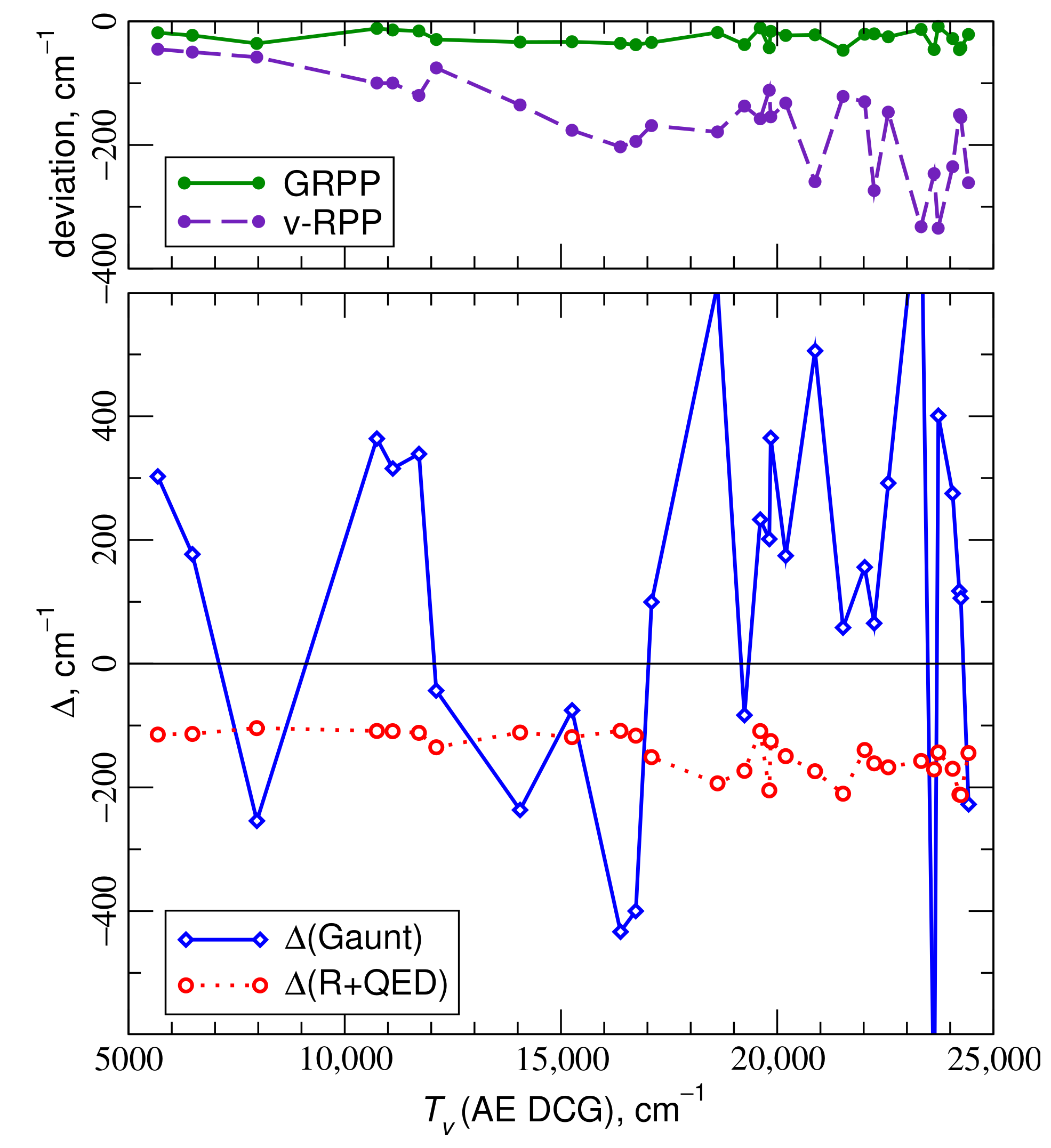
4.1. Electronic States of the ThO Molecule

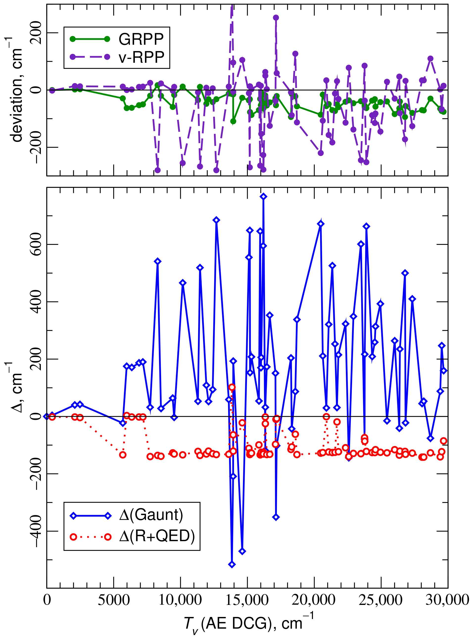
The vertical excitation spectrum of the ThO molecule was calculated at the experimental ground-state internuclear separation, $R_e=1.840$ Å [89], using the intermediate-Hamiltonian Fock space relativistic coupled cluster method (IH-FS-RCC) [28] within the singles-and-doubles approximation (CCSD) to solve the many-electron problem. All electrons except for those of Th shells with $n\le 4$ and $1s$-shell of O were correlated. The vacuum state and one-electron spinors were defined by the solutions of the Hartree–Fock problem for the ground state of the closed-shell ThO${}^{2+}$ ion whereas the target states of the neutral ThO molecule were treated within the two-particle $\left(0h2p\right)$ Fock space sector. All-electron Dirac–Coulomb and Dirac–Coulomb–Gaunt calculations were performed using the non-contracted s, p, d and f components of Dyall’s thorium quadruple-zeta basis [90] augmented with a single f-function manifold (exponential parameter 0.050404710) and $\left(7g6h5i\right)/\left[5g4h3i\right]$ scalar-relativistic averaged atomic natural orbitals (see Supplementary Materials). For the oxygen atom, a relativistic recontraction [91] of the aug-cc-pVQZ basis sets [92,93] was employed. The GRPP-adapted equivalent of the all-electron Th basis set was obtained by rejecting the most compact and reoptimizing several largest exponential parameters of the remainder $spdf$ functions, keeping untouched high-angular-momentum components (all parameters are provided in Supplementary Materials); the same basis for oxygen was used along with the empty-core GRPP [58] for this atom. The complete model space at the FS-RCC stage was defined by 24 Kramers pairs of lowest-energy virtual spinors of ThO${}^{2+}$; the incomplete main model space [28] for the $\left(0h2p\right)$ sector was spanned by all distributions of two active electrons among 6 lowest-energy pairs (roughly corresponding to $7s$ and $6d$ atomic spinors of Th) and all determinants with orbital energy sums in the same range. The algorithm defining the intermediate-state shift parameters was described in detail previously for the Ra atom and Tl${}^{+}$, Lu${}^{+}$ atomic ions in Ref. [28]. For 31 lowest-energy eigenvectors of the intermediate Hamiltonian (excitation energies up to ca. 25,000 cm${}^{-1}$), the fractions within the main model space exceed 95%, indicating the adequacy of the chosen intermediate-Hamiltonian scheme for the corresponding electronic states.

The resulting vertical excitation energies $T_v$ evaluated with different relativistic Hamiltonians are compared in Figure 7. The deviation of $T_v$ values obtained with GRPP/Gaunt from the corresponding results of all-electron calculations with Dirac–Coulomb–Gaunt Hamiltonian employing the X2C MMF transformation [6] ($T_v\left(\mathrm{AE}\mathrm{DCG}\right)$) are always less than 50 cm${}^{-1}$ (rms deviation 29 cm${}^{-1}$). This deviation is significantly smaller than the contribution of retardation and QED effects to excitation energies ($\Delta$(R+QED)) estimated as the difference between the results of calculations with GRPP/QED and GRPP/Gaunt (104–212 cm${}^{-1}$; note that the contribution arising from the use of different finite nuclear models in GRPP/QED and GRPP/Gaunt is negligibly small, less than one wavenumber). It is thus clear that the use of the tiny-core GRPP/QED approach should be preferred to the all-electron Dirac–Coulomb–Gaunt model not only because of significant computational savings, but also for reasons of accuracy. As follows from the magnitudes of contributions from Gaunt interactions (Figure 7, bottom), one can make an even stronger statement concerning the reliability of the GRPP/QED model versus the Dirac–Coulomb one. The replacement of the full GRPP/Gaunt by its valence semilocal component (v-RPP) leads to a significant deterioration of results (the deviation of v-RPP/Gaunt excitation energies from their all-electron counterparts can exceed 300 cm${}^{-1}$), so that the incorporation of interactions beyond the Dirac–Coulomb–Gaunt approximations into semilocal pseudopotentials hardly seems reasonable, except for the cases of s and p block elements.

4.2. Electronic States of the UO${}_2$ Molecule

The UO${}_2$ molecule is an example of a heavy polyatomic molecule with a quite diverse set of electronic states. It was extensively studied both theoretically and experimentally in the last two decades (see [94,95,96,97,98] and references therein).

In the present work, the vertical excitation spectrum of UO${}_2$ was calculated for the linear geometry and at the experimental ground-state internuclear separation $R_e(\mathrm{U}-\mathrm{O})=1.790$ Å [98]. Low-lying electronic states of UO${}_2$ can be accessed in the $\left(0h2p\right)$ Fock space sector. The IH-FS-RCCSD method with single and double excitations was used [28]. The complete model space was defined by 24 Kramers pairs of lowest-energy virtual spinors of the closed-shell UO${}_2^{2+}$ ion. The thorough analysis [95] of the composition of electronic states below 30,000 cm${}^{-1}$ shows that all these states can be obtained within the incomplete main model space intermediate-Hamiltonian technique. For this purpose, we split the manifold of virtual active spinors of UO${}_2^{2+}$ into three groups (the notation is adopted from [95], see this paper for the detailed picture of one-electron states): (a) $7s_{1/2g}^{\sigma }$, $5f_{5/2u}^{\varphi }$, $6d_{3/2g}^{\delta }$, $5f_{3/2u}^{\delta }$, $6d_{5/2g}^{\delta }$, $5f_{7/2u}^{\varphi }$, $5f_{5/2u}^{\delta }$ spinors; (b) $5f_{1/2u}^{\pi }$, $5f_{3/2u}^{\pi }$, $7p_{1/2u}^{\pi }$, $7p_{3/2u}^{\pi }$, $6d_{1/2g}^{\pi }$, $6d_{3/2g}^{\pi }$, $5f_{1/2u}^{\sigma }$, $7p_{1/2u}^{\sigma }$ spinors; and (c) the remaining set of virtual active spinors are used as buffer ones. Wavefunctions of target states are dominated either by determinants with two electrons distributed over spinors from the first group or by determinants with one electron on the first group spinor and the other electron on the second group spinor. The adequacy of the chosen IH model is confirmed by the fact that for 79 electronic states below 30,000 cm${}^{-1}$ fractions of main model space determinants exceed 94%. All-electron Dirac–Coulomb and Dirac–Coulomb–Gaunt calculations were performed within the exact two-component molecular mean field (X2C MMF) approximation [6]. The basis set for U was derived from the exponents from the Dyall’s quadruple-zeta basis set [90] for the s, p, d, and f functions and then augmented with ($7g6h4i$)/[$5g4h3i$] scalar-relativistic atomic natural orbitals (see Supplementary Materials). For the pseudopotential calculations, the most compact primitive Gaussian functions were rejected, keeping untouched high-angular-momentum (g, h, i) functions. For the O atom, the aug-cc-pVQZ-DK basis set [91] was used in both all-electron and RPP calculations; in the latter case, the empty-core (no core electrons) pseudopotential of Mosyagin et al. [58] was also used. Shells of U with the principal quantum number $n\le$ 4 as well as the $1s$ shell of O were frozen at the IH-FS-RCC stage.

The resulting vertical excitation energies evaluated with different relativistic Hamiltonians are compared in Figure 8. The patterns are pretty similar to those obtained for the ThO molecule (Section 4.1). The deviation of GRPP/Gaunt excitation energies from the reference DCG values does not exceed 110 cm${}^{-1}$ (rms deviation 51 cm${}^{-1}$, mean absolute error 45 cm${}^{-1}$). This is larger than for ThO, but is fully consistent with estimates at the SCF level. One can see from Tables S1 and S2 in the Supplementary materials that the GRPP errors are naturally arranged according to the changes in the occupation number of the $5f$ shell. Thus, in the case of uranium and its ions these errors are of the order of +50 cm${}^{-1}$ for the transitions with the decrease of this occupation number by one (and the rough proportionality holds for the other transitions), whereas they are within 10 cm${}^{-1}$ for the transitions without the change in this occupation number. Similarly to the case of ThO, the error introduced by the GRPP approximation is smaller than the contribution of retardation and QED effects (up to 140 cm${}^{-1}$). It is worth noting that the $\Delta$(R+QED) contribution strongly depends on the fraction of configurations involving the $7s_{1/2g}^{\sigma }$ spinor ($\sim +120$ cm${}^{-1}$ per one electron). In particular, the dropdown value of $\Delta$(R+QED)$=+102$ cm${}^{-1}$ corresponds to the (2)$0_g$ state dominated by the ${\left(7s_{1/2g}^{\sigma }\right)}^2$ configuration. It should be emphasized that Gaunt contributions to the excitation energies considered (reaching 767 cm${}^{-1}$, rms deviation 316 cm${}^{-1}$) exceed the GRPP error by an order of magnitude (Figure 8, bottom). This clearly indicates that the use of the four-component Dirac–Coulomb approximation does not make sense for this system and should not be preferred over the tiny-core pseudopotential approach. Note that even for the conventional semilocal (valence) RPP maximal deviation is twice smaller (345 cm${}^{-1}$) than for the DC Hamiltonian.

5. Conclusions

The version of the LIBGRPP library presented in this paper provides universal tools for the evaluation of all types of molecular integrals arising within the generalized relativistic pseudopotential (GRPP) model.

The numerical scheme for integrals over the local term of the pseudopotential based on the one-center re-expansion of basis functions is not recommended due to severe numerical instabilities arising for large values of exponential parameters in Gaussian basis functions. This problem can be overcome by switching to other computational scheme based on numerically stable recurrence relations analogous to the McMurchie–Davidson relations for nuclear attraction integrals.

It should be pointed out that the semi-numerical scheme used in the present work to evaluate integrals with projectors after some modifications can be used to calculate molecular integrals over any arbitrary atom-centered potential. An important example of such an operator is the electrostatic potential generated by some finite nuclear charge distribution, e.g., the Fermi distribution [99,100], which is not currently available for molecular calculations due to the absence of corresponding nuclear attraction integrals in electronic structure packages. Such a feature will be demanded in the framework of four-component relativistic calculations on superheavy element compounds. The other example of such a non-local potential is the model Lamb shift operator [18,64].

Pilot applications of the developed LIBGRPP library in conjunction with the relativistic coupled cluster theory to electronic transitions in the ThO and UO${}_2$ molecules clearly demonstrate that the rather economical tiny-core pseudopotential model can exceed in accuracy relativistic all-electron models defined by Dirac–Coulomb Hamiltonian in describing electronic excitations in f-block element compounds. Deviations of excitation energies obtained within the GRPP approach from their all-electron Dirac–Coulomb–Gaunt counterparts do not exceed 50 cm${}^{-1}$ (rms deviation 29 cm${}^{-1}$) for the 31 lowest-energy states of ThO and 110 cm${}^{-1}$ (rms deviation 51 cm${}^{-1}$) for the 79 states of UO${}_2$. Generalized pseudopotentials also provide an attractive opportunity to include QED and Breit effects into the relativistic electronic structure model completely at no cost. Further experiences with the GRPP model are desirable to elucidate its capabilities in molecular problems and its scope of applicability.

There could be some possible future developments that are expected to improve the code of the library and extend the scope of its applicability. In particular, the use of more efficient radial quadratures and more robust schemes for pre-screening of radial integrals (like that developed in [75,76]) appears to be the most promising direction for further developments. It also seems reasonable to provide the Python interface to LIBGRPP routines to increase interoperability with modern electronic structure packages like PySCF [101]. The other possible direction of future work will address further integration with solid-matter quantum chemistry codes in order to explore the power of the generalized relativistic pseudopotential model not only in atomic and molecular, but also in solid state problems [102,103,104]. We finally note that the computational scheme of evaluation of integrals over GRPP-specific non-local terms presented in the paper does not actually introduce any fundamentally new types of RPP integrals. Thus, it can be readily implemented within any existing code for pseudopotential integration (given that the code for overlap integrals is naturally presented in almost every quantum chemistry package). This paves the way to routine calculations with one of the most comprehensive relativistic Hamiltonians at the moment, completely bypassing any complicated four-component calculations.

References

1. Eliav, E.; Kaldor, U. Study of actinides by relativistic coupled cluster methods. In Computational Methods in Lanthanide and Actinide Chemistry; John Wiley & Sons, Ltd.: Hoboken, NJ, USA, 2015; Chapter 2; pp. 23–54. [Google Scholar] [CrossRef]
2. Eliav, E.; Fritzsche, S.; Kaldor, U. Electronic structure theory of the superheavy elements. Nucl. Phys. 2015, 944, 518–550. [Google Scholar] [CrossRef]
3. Eliav, E.; Borschevsky, A.; Kaldor, U. High-accuracy relativistic coupled-cluster calculations for the heaviest elements. In Handbook of Relativistic Quantum Chemistry; Liu, W., Ed.; Springer: Berlin/Heidelberg, Germany, 2017; pp. 825–855. [Google Scholar] [CrossRef]
4. Eliav, E.; Borschevsky, A.; Zaitsevskii, A.; Oleynichenko, A.V.; Kaldor, U. Relativistic Fock-space coupled cluster method: Theory and recent applications. In Reference Module in Chemistry, Molecular Sciences and Chemical Engineering; Elsevier: Amsterdam, The Netherlands, 2022. [Google Scholar] [CrossRef]
5. Dyall, K.; Faegri, K. Introduction to Relativistic Quantum Chemistry; Oxford University Press: Oxford, UK, 2007. [Google Scholar]
6. Sikkema, J.; Visscher, L.; Saue, T.; Iliaš, M. The molecular mean-field approach for correlated relativistic calculations. J. Chem. Phys. 2009, 131, 124116. [Google Scholar] [CrossRef] [PubMed]
7. Saue, T. Relativistic Hamiltonians for chemistry: A primer. Chem. Phys. Chem. 2011, 12, 3077–3094. [Google Scholar] [CrossRef] [PubMed]
8. Bratsev, V.F.; Deyneka, G.B.; Tupitsyn, I.I. Application of the Hartree-Fock method to calculation of relativistic atomic wave functions. Bull. Acad. Sci. USSR Phys. Ser. 1977, 41, 173–182. [Google Scholar]
9. Parpia, F.A.; Froese Fischer, C.; Grant, I.P. GRASP92: A package for large-scale relativistic atomic structure calculations. Comput. Phys. Commun. 1996, 94, 249–271. [Google Scholar] [CrossRef]
10. Kozlov, M.; Porsev, S.; Safronova, M.S.; Tupitsyn, I. CI-MBPT: A package of programs for relativistic atomic calculations based on a method combining configuration interaction and many-body perturbation theory. Comput. Phys. Commun. 2015, 195, 199–213. [Google Scholar] [CrossRef] [Green Version]
11. Kahl, E.V.; Berengut, J.C. AMBiT: A programme for high-precision relativistic atomic structure calculations. Comput. Phys. Commun. 2019, 238, 232–243. [Google Scholar] [CrossRef] [Green Version]
12. Fritzsche, S. A fresh computational approach to atomic structures, processes and cascades. Comput. Phys. Commun. 2019, 240, 1–14. [Google Scholar] [CrossRef]
13. Visscher, L.; Visser, O.; Aerts, P.J.C.; Merenga, H.; Nieuwpoort, W.C. Relativistic quantum chemistry: The MOLFDIR program package. Comput. Phys. Commun. 1994, 81, 120–144. [Google Scholar] [CrossRef]
14. Liu, W.; Wang, F.; Li, L. The Beijing Density Functional (BDF) program package: Methodologies and applications. J. Theor. Comput. Chem. 2003, 2, 257–272. [Google Scholar] [CrossRef]
15. Van Wüllen, C. A quasirelativistic two-component density Functional and Hartree-Fock program. In Progress in Physical Chemistry Volume 3; Oldenbourg Wissenschaftsverlag GmbH: Munich, Germany, 2010; pp. 123–136. [Google Scholar] [CrossRef]
16. Saue, T.; Bast, R.; Gomes, A.S.P.; Jensen, H.J.A.; Visscher, L.; Aucar, I.A.; Di Remigio, R.; Dyall, K.G.; Eliav, E.; Fasshauer, E.; et al. The DIRAC code for relativistic molecular calculations. J. Chem. Phys. 2020, 152, 204104. [Google Scholar] [CrossRef]
17. Repisky, M.; Komorovsky, S.; Kadek, M.; Konecny, L.; Ekström, U.; Malkin, E.; Kaupp, M.; Ruud, K.; Malkina, O.L.; Malkin, V.G. ReSpect: Relativistic spectroscopy DFT program package. J. Chem. Phys. 2020, 152, 184101. [Google Scholar] [CrossRef]
18. Shabaev, V.M.; Tupitsyn, I.I.; Yerokhin, V.A. Model operator approach to the Lamb shift calculations in relativistic many-electron atoms. Phys. Rev. A 2013, 88, 012513. [Google Scholar] [CrossRef] [Green Version]
19. Eliav, E.; Kaldor, U. Relativistic Four-Component Multireference Coupled Cluster Methods: Towards A Covariant Approach. In Recent Progress in Coupled Cluster Methods: Theory and Applications; Cársky, P., Paldus, J., Pittner, J., Eds.; Springer: Dordrecht, The Netherlands, 2010; pp. 113–144. [Google Scholar] [CrossRef]
20. Thierfelder, C.; Schwerdtfeger, P. Quantum electrodynamic corrections for the valence shell in heavy many-electron atoms. Phys. Rev. A 2010, 82, 062503. [Google Scholar] [CrossRef]
21. Roberts, B.M.; Dzuba, V.A.; Flambaum, V.V. Quantum electrodynamics corrections to energies, transition amplitudes, and parity nonconservation in Rb, Cs, Ba+, Tl, Fr, and Ra+. Phys. Rev. A 2013, 87, 054502. [Google Scholar] [CrossRef] [Green Version]
22. Lindgren, I. Relativistic Many-Body Theory. A New Field-Theoretical Approach, 2nd ed.; Springer: Berlin/Heidelberg, Germany, 2016. [Google Scholar] [CrossRef]
23. Sunaga, A.; Saue, T. Towards highly accurate calculations of parity violation in chiral molecules: Relativistic coupled-cluster theory including QED-effects. Mol. Phys. 2021, 119, e1974592. [Google Scholar] [CrossRef]
24. Sunaga, A.; Salman, M.; Saue, T. 4-component relativistic Hamiltonian with effective QED potentials for molecular calculations. J. Chem. Phys. 2022, 157, 164101. [Google Scholar] [CrossRef]
25. Kaygorodov, M.Y.; Usov, D.P.; Eliav, E.; Kozhedub, Y.S.; Malyshev, A.V.; Oleynichenko, A.V.; Shabaev, V.M.; Skripnikov, L.V.; Titov, A.V.; Tupitsyn, I.I.; et al. Ionization potentials and electron affinities of Rg, Cn, Nh, and Fl superheavy elements. Phys. Rev. A 2022, 105, 062805. [Google Scholar] [CrossRef]
26. Petrov, A.N.; Mosyagin, N.S.; Titov, A.V.; Tupitsyn, I.I. Accounting for the Breit interaction in relativistic effective core potential calculations of actinides. J. Phys. B 2004, 37, 4621–4637. [Google Scholar] [CrossRef]
27. Skripnikov, L.V.; Chubukov, D.V.; Shakhova, V.M. The role of QED effects in transition energies of heavy-atom alkaline earth monofluoride molecules: A theoretical study of Ba+, BaF, RaF, and E120F. J. Chem. Phys. 2021, 155, 144103. [Google Scholar] [CrossRef]
28. Zaitsevskii, A.; Mosyagin, N.S.; Oleynichenko, A.V.; Eliav, E. Generalized relativistic small-core pseudopotentials accounting for quantum electrodynamic effects: Construction and pilot applications. arXiv 2022, arXiv:2208.12296. [Google Scholar] [CrossRef]
29. Knecht, S.; Repisky, M.; Jensen, H.J.A.; Saue, T. Exact two-component Hamiltonians for relativistic quantum chemistry: Two-electron picture-change corrections made simple. J. Chem. Phys. 2022, 157, 114106. [Google Scholar] [CrossRef] [PubMed]
30. Seijo, L.; Barandiarán, Z. Relativistic ab-initio model potential calculations for molecules and embedded clusters. Theor. Comput. Chem. 2004, 14, 417–475. [Google Scholar] [CrossRef]
31. Abarenkov, I.V.; Heine, V. The model potential for positive ions. Philos. Mag. 1965, 12, 529–537. [Google Scholar] [CrossRef]
32. Christiansen, P.A.; Lee, Y.S.; Pitzer, K.S. Improved ab initio effective core potentials for molecular calculations. J. Chem. Phys. 1979, 71, 4445–4450. [Google Scholar] [CrossRef]
33. Titov, A.V.; Mosyagin, N.S. Generalized relativistic effective core potential: Theoretical grounds. Int. J. Quantum Chem. 1999, 71, 359–401. [Google Scholar] [CrossRef]
34. Schwerdtfeger, P. The pseudopotential approximation in electronic structure theory. Chem. Phys. Chem. 2011, 12, 3143–3155. [Google Scholar] [CrossRef]
35. Dolg, M.; Cao, X. Relativistic pseudopotentials: Their development and scope of applications. Chem. Rev. 2012, 112, 403–480. [Google Scholar] [CrossRef]
36. Mosyagin, N.S.; Zaitsevskii, A.V.; Skripnikov, L.V.; Titov, A.V. Generalized relativistic effective core potentials for actinides. Int. J. Quantum Chem. 2016, 116, 301–315. [Google Scholar] [CrossRef] [Green Version]
37. Mosyagin, N.S.; Zaitsevskii, A.V.; Titov, A.V. Generalized relativistic effective core potentials for superheavy elements. Int. J. Quantum Chem. 2020, 120, e26076. [Google Scholar] [CrossRef]
38. Lee, Y.S.; Ermler, W.C.; Pitzer, K.S. Ab initio effective core potentials including relativistic effects. I. Formalism and applications to the Xe and Au atoms. J. Chem. Phys. 1977, 67, 5861–5876. [Google Scholar] [CrossRef]
39. Hafner, P.; Schwarz, W. Molecular spinors from the quasi-relativistic pseudopotential approach. Chem. Phys. Lett. 1979, 65, 537–541. [Google Scholar] [CrossRef]
40. Pitzer, R.M.; Winter, N.W. Spin-orbit (core) and core potential integrals. Int. J. Quantum Chem. 1991, 40, 773–780. [Google Scholar] [CrossRef]
41. Pacios, L.F.; Christiansen, P.A. Ab initio relativistic effective potentials with spin-orbit operators. I. Li through Ar. J. Chem. Phys. 1985, 82, 2664–2671. [Google Scholar] [CrossRef]
42. Hurley, M.M.; Pacios, L.F.; Christiansen, P.A.; Ross, R.B.; Ermler, W.C. Ab initio relativistic effective potentials with spin-orbit operators. II. K through Kr. J. Chem. Phys. 1986, 84, 6840–6853. [Google Scholar] [CrossRef]
43. LaJohn, L.A.; Christiansen, P.A.; Ross, R.B.; Atashroo, T.; Ermler, W.C. Ab initio relativistic effective potentials with spin–orbit operators. III. Rb through Xe. J. Chem. Phys. 1987, 87, 2812–2824. [Google Scholar] [CrossRef]
44. Ross, R.B.; Powers, J.M.; Atashroo, T.; Ermler, W.C.; LaJohn, L.A.; Christiansen, P.A. Ab initio relativistic effective potentials with spin–orbit operators. IV. Cs through Rn. J. Chem. Phys. 1990, 93, 6654–6670. [Google Scholar] [CrossRef]
45. Pacios, L.F.; Olcina, V.B. Modified Ar core ab initio relativistic effective potentials for transition metals Sc through Cu. J. Chem. Phys. 1991, 95, 441–450. [Google Scholar] [CrossRef]
46. Ermler, W.C.; Ross, R.B.; Christiansen, P.A. Ab initio relativistic effective potentials with spin-orbit operators. VI. Fr through Pu. Int. J. Quantum Chem. 1991, 40, 829–846. [Google Scholar] [CrossRef]
47. Ross, R.B.; Gayen, S.; Ermler, W.C. Ab initio relativistic effective potentials with spin-orbit operators. V. Ce through Lu. J. Chem. Phys. 1994, 100, 8145–8155. [Google Scholar] [CrossRef]
48. Wildman, S.A.; DiLabio, G.A.; Christiansen, P.A. Accurate relativistic effective potentials for the sixth-row main group elements. J. Chem. Phys. 1997, 107, 9975–9979. [Google Scholar] [CrossRef]
49. Nash, C.S.; Bursten, B.E.; Ermler, W.C. Ab initio relativistic potentials with spin-orbit operators. VII. Am through element 118. J. Chem. Phys. 1997, 106, 5133–5142, Erratum in J. Chem. Phys. 1999, 111, 2347. [Google Scholar] [CrossRef]
50. Cundari, T.R.; Stevens, W.J. Effective core potential methods for the lanthanides. J. Chem. Phys. 1993, 98, 5555–5565. [Google Scholar] [CrossRef]
51. Hay, P.J.; Wadt, W.R. Ab initio effective core potentials for molecular calculations. Potentials for K to Au including the outermost core orbitals. J. Chem. Phys. 1985, 82, 299–310. [Google Scholar] [CrossRef]
52. Dolg, M.; Cao, X. Accurate relativistic small-core pseudopotentials for actinides. Energy adjustment for uranium and first applications to uranium hydride. J. Phys. Chem. A 2009, 113, 12573–12581. [Google Scholar] [CrossRef]
53. Mosyagin, N.S.; Zaitsevskii, A.; Titov, A.V. Shape-consistent relativistic effective potentials of small atomic cores. Int. Rev. At. Mol. Phys. 2010, 1, 63–72. [Google Scholar]
54. Mosyagin, N.S. Generalized relativistic effective core potentials for lanthanides. Nonlinear Phenom. Complex Syst. 2017, 20, 111–132. [Google Scholar]
55. Tupitsyn, I.I.; Mosyagin, N.S.; Titov, A.V. Generalized relativistic effective core potential. I. Numerical calculations for atoms Hg through Bi. J. Chem. Phys. 1995, 103, 6548–6555. [Google Scholar] [CrossRef]
56. Mosyagin, N.S.; Titov, A.V.; Latajka, Z. Generalized relativistic effective core potential: Gaussian expansions of potentials and pseudospinors for atoms Hg through Rn. Int. J. Quantum Chem. 1997, 63, 1107–1122. [Google Scholar] [CrossRef]
57. Mosyagin, N.S.; Titov, A.V.; Eliav, E.; Kaldor, U. Generalized relativistic effective core potential and relativistic coupled cluster calculation of the spectroscopic constants for the HgH molecule and its cation. J. Chem. Phys. 2001, 115, 2007–2013. [Google Scholar] [CrossRef]
58. Mosyagin, N.; Oleynichenko, A.; Zaitsevskii, A.; Kudrin, A.; Pazyuk, E.; Stolyarov, A. Ab initio relativistic treatment of the a3Π − X1 Σ+, a′3Σ+X1Σ+ and A1Π − X1Σ+ systems of the CO molecule. J. Quant. Spectrosc. Radiat. Transf. 2021, 263, 107532. [Google Scholar] [CrossRef]
59. Zaitsevskii, A.; Skripnikov, L.V.; Mosyagin, N.S.; Isaev, T.; Berger, R.; Breier, A.A.; Giesen, T.F. Accurate ab initio calculations of RaF electronic structure appeal to more laser-spectroscopical measurements. J. Chem. Phys. 2022, 156, 044306. [Google Scholar] [CrossRef]
60. Titov, A.V.; Petrov, A.N.; Panin, A.I.; Khait, Y.G. MOLGEP Code for Calculation of Matrix Elements with GRECP (St.-Petersburg, 1999).
61. McMurchie, L.E.; Davidson, E.R. Calculation of integrals over ab initio pseudopotentials. J. Comput. Phys. 1981, 44, 289–301. [Google Scholar] [CrossRef] [Green Version]
62. Park, Y.C.; Lee, Y.S. Two-component spin-orbit effective core potential calculations with an all-electron relativistic program DIRAC. Bull. Korean Chem. Soc. 2012, 33, 803–808. [Google Scholar] [CrossRef] [Green Version]
63. Mitin, A.V.; Van Wüllen, C. Two-component relativistic density-functional calculations of the dimers of the halogens from bromine through element 117 using effective core potential and all-electron methods. J. Chem. Phys. 2006, 124, 064305. [Google Scholar] [CrossRef]
64. Shabaev, V.M.; Tupitsyn, I.I.; Yerokhin, V.A. QEDMOD: Fortran program for calculating the model Lamb-shift operator. Comput. Phys. Commun. 2018, 223, 69. [Google Scholar] [CrossRef]
65. Generalized Relativistic Pseudopotentials. Available online: http://qchem.pnpi.spb.ru/recp (accessed on 2 January 2023).
66. Helgaker, T.; Jørgensen, P.; Olsen, J. Molecular Electronic-Structure Theory; Wiley: New York, NY, USA, 2000. [Google Scholar] [CrossRef]
67. Van Wüllen, C. Numerical instabilities in the computation of pseudopotential matrix elements. J. Comput. Chem. 2005, 27, 135–141. [Google Scholar] [CrossRef]
68. McMurchie, L.E.; Davidson, E.R. One- and two-electron integrals over Cartesian Gaussian functions. J. Comput. Phys. 1978, 26, 218–231. [Google Scholar] [CrossRef] [Green Version]
69. Jensen, J.O.; Carrieri, A.H.; Vlahacos, C.P.; Zeroka, D.; Hameka, H.F.; Merrow, C.N. Evaluation of one-electron integrals for arbitrary operators V(r) over Cartesian Gaussians: Application to inverse-square distance and Yukawa operators. J. Comput. Chem. 1993, 14, 986–994. [Google Scholar] [CrossRef]
70. Gao, B.; Thorvaldsen, A.J.; Ruud, K. GEN1INT: A unified procedure for the evaluation of one-electron integrals over Gaussian basis functions and their geometric derivatives. Int. J. Quantum Chem. 2011, 111, 858–872. [Google Scholar] [CrossRef]
71. Skylaris, C.K.; Gagliardi, L.; Handy, N.C.; Ioannou, A.G.; Spencer, S.; Willetts, A.; Simper, A.M. An efficient method for calculating effective core potential integrals which involve projection operators. Chem. Phys. Lett. 1998, 296, 445–451. [Google Scholar] [CrossRef] [Green Version]
72. Flores-Moreno, R.; Alvarez-Mendez, R.J.; Vela, A.; Köster, A.M. Half-numerical evaluation of pseudopotential integrals. J. Comput. Chem. 2006, 27, 1009–1019. [Google Scholar] [CrossRef] [PubMed]
73. Mura, M.E.; Knowles, P.J. Improved radial grids for quadrature in molecular density-functional calculations. J. Chem. Phys. 1996, 104, 9848–9858. [Google Scholar] [CrossRef]
74. Lindh, R.; Malmqvist, P.Å.; Gagliardi, L. Molecular integrals by numerical quadrature. I. Radial integration. Theor. Chim. Acta 2001, 106, 178–187. [Google Scholar] [CrossRef] [Green Version]
75. Song, C.; Wang, L.P.; Sachse, T.; Preiss, J.; Presselt, M.; Martinez, T.J. Efficient implementation of effective core potential integrals and gradients on graphical processing units. J. Chem. Phys. 2015, 143, 014114. [Google Scholar] [CrossRef] [Green Version]
76. McKenzie, S.C.; Epifanovsky, E.; Barca, G.M.J.; Gilbert, A.T.B.; Gill, P.M.W. Efficient method for calculating effective core potential integrals. J. Phys. Chem. A 2018, 122, 3066–3075. [Google Scholar] [CrossRef]
77. Shaw, R.A.; Hill, J.G. Prescreening and efficiency in the evaluation of integrals over ab initio effective core potentials. J. Chem. Phys. 2017, 147, 074108. [Google Scholar] [CrossRef] [Green Version]
78. McKenzie, S.C. Efficient Computation of Integrals in Modern Correlated Methods. Ph.D. Thesis, Faculty of Science, University of Sydney, Sydney, Australia, 2020. [Google Scholar]
79. Galassi, M.; Davies, J.; Theiler, J.; Gough, B.; Jungman, G. GNU Scientific Library-Reference Manual, Third Edition, for GSL Version 1.12, 3rd ed.; Network Theory Ltd.: London, UK, 2009. [Google Scholar]
80. Obara, S.; Saika, A. Efficient recursive computation of molecular integrals over Cartesian Gaussian functions. J. Chem. Phys. 1986, 84, 3963–3974. [Google Scholar] [CrossRef]
81. Gomes, A.S.P.; Saue, T.; Visscher, L.A.; Jensen, H.J.; Bast, R.; Aucar, I.A.; Bakken, V.; Dyall, K.G.; Dubillard, S.; Ekstroem, U.; et al. DIRAC, a Relativistic Ab Initio Electronic Structure Program, Release DIRAC19. 2019. Available online: http://diracprogram.org (accessed on 17 December 2022).
82. Skripnikov, L.V.; Petrov, A.N.; Mosyagin, N.S.; Ezhov, V.F.; Titov, A.V. Ab initio calculation of the spectroscopic properties of TlF. Opt. Spectrosc. 2009, 106, 790–792. [Google Scholar] [CrossRef]
83. Isaev, T.A.; Mosyagin, N.S.; Petrov, A.N.; Titov, A.V. In search of the electron electric dipole moment: Relativistic correlation calculations of the P,T-violation effect in the ground state of HI+. Phys. Rev. Lett. 2005, 95, 163004. [Google Scholar] [CrossRef] [Green Version]
84. Mosyagin, N.S.; Isaev, T.A.; Titov, A.V. Is E112 a relatively inert element? Benchmark relativistic correlation study of spectroscopic constants in E112H and its cation. J. Chem. Phys. 2006, 124, 224302. [Google Scholar] [CrossRef] [Green Version]
85. Kudashov, A.D.; Petrov, A.N.; Skripnikov, L.V.; Mosyagin, N.S.; Isaev, T.A.; Berger, R.; Titov, A.V. Ab initio study of radium monofluoride (RaF) as a candidate to search for parity- and time-and-parity–violation effects. Phys. Rev. A 2014, 90, 052513. [Google Scholar] [CrossRef] [Green Version]
86. Oleynichenko, A.V.; Zaitsevskii, A.; Eliav, E. Towards high performance relativistic electronic structure modelling: The EXP-T program package. In Proceedings of the Supercomputing; Voevodin, V., Sobolev, S., Eds.; Springer International Publishing: Cham, Switzerland, 2020; Volume 1331, pp. 375–386. [Google Scholar] [CrossRef]
87. Oleynichenko, A.V.; Zaitsevskii, A.; Skripnikov, L.V.; Eliav, E. Relativistic Fock space coupled cluster method for many-electron systems: Non-perturbative account for connected triple excitations. Symmetry 2020, 12, 1101. [Google Scholar] [CrossRef]
88. Oleynichenko, A.; Zaitsevskii, A.; Eliav, E. EXP-T, an Extensible Code for Fock Space Relativistic Coupled Cluster Calculations. 2022. Available online: http://www.qchem.pnpi.spb.ru/expt (accessed on 17 December 2022).
89. Dewberry, C.T.; Etchison, K.C.; Cooke, S.A. The pure rotational spectrum of the actinide-containing compound thorium monoxide. Phys. Chem. Chem. Phys. 2007, 9, 4895. [Google Scholar] [CrossRef]
90. Dyall, K.G. Relativistic double-zeta, triple-zeta, and quadruple-zeta basis sets for the actinides Ac–Lr. Theor. Chem. Acc. 2007, 117, 491–500. [Google Scholar] [CrossRef]
91. De Jong, W.A.; Harrison, R.J.; Dixon, D.A. Parallel Douglas-Kroll energy and gradients in NWChem: Estimating scalar relativistic effects using Douglas-Kroll contracted basis sets. J. Chem. Phys. 2001, 114, 48. [Google Scholar] [CrossRef]
92. Dunning, T.H. Gaussian basis sets for use in correlated molecular calculations. I. The atoms boron through neon and hydrogen. J. Chem. Phys. 1989, 90, 1007–1023. [Google Scholar] [CrossRef]
93. Kendall, R.A.; Dunning, T.H., Jr.; Harrison, R.J. Electron affinities of the first-row atoms revisited. Systematic basis sets and wave functions. J. Chem. Phys. 1992, 96, 6796. [Google Scholar] [CrossRef] [Green Version]
94. Gagliardi, L.; Heaven, M.C.; Krogh, J.W.; Roos, B.O. The electronic spectrum of the UO2 molecule. J. Am. Chem. Soc. 2004, 127, 86–91. [Google Scholar] [CrossRef] [Green Version]
95. Infante, I.; Eliav, E.; Vilkas, M.J.; Ishikawa, Y.; Kaldor, U.; Visscher, L. A Fock space coupled cluster study on the electronic structure of the UO2, UO2+, U4+, and U5+ species. J. Chem. Phys. 2007, 127, 124308. [Google Scholar] [CrossRef]
96. Li, W.L.; Su, J.; Jian, T.; Lopez, G.V.; Hu, H.S.; Cao, G.J.; Li, J.; Wang, L.S. Strong electron correlation in UO2: A photoelectron spectroscopy and relativistic quantum chemistry study. J. Chem. Phys. 2014, 140, 094306. [Google Scholar] [CrossRef] [PubMed] [Green Version]
97. Czekner, J.; Lopez, G.V.; Wang, L.S. High resolution photoelectron imaging of UO and UO2 and the low-lying electronic states and vibrational frequencies of UO and UO2. J. Chem. Phys. 2014, 141, 244302. [Google Scholar] [CrossRef] [PubMed] [Green Version]
98. Kovács, A.; Konings, R.J.M.; Gibson, J.K.; Infante, I.; Gagliardi, L. Quantum chemical calculations and experimental investigations of molecular actinide oxides. Chem. Rev. 2015, 115, 1725–1759. [Google Scholar] [CrossRef] [PubMed]
99. Parpia, F.A.; Mohanty, A.K. Relativistic basis-set calculations for atoms with Fermi nuclei. Phys. Rev. A 1992, 46, 3735–3745. [Google Scholar] [CrossRef] [PubMed]
100. Visscher, L.; Dyall, K.G. Dirac-Fock atomic electronic structure calculations using different nuclear charge distributions. At. Data Nucl. Data Tables 1997, 67, 207–224. [Google Scholar] [CrossRef]
101. Sun, Q.; Zhang, X.; Banerjee, S.; Bao, P.; Barbry, M.; Blunt, N.S.; Bogdanov, N.A.; Booth, G.H.; Chen, J.; Cui, Z.H.; et al. Recent developments in the PySCF program package. J. Chem. Phys. 2020, 153, 024109. [Google Scholar] [CrossRef]
102. Lomachuk, Y.V.; Maltsev, D.A.; Mosyagin, N.S.; Skripnikov, L.V.; Bogdanov, R.V.; Titov, A.V. Compound-tunable embedding potential: Which oxidation state of uranium and thorium as point defects in xenotime is favorable? Phys. Chem. Chem. Phys. 2020, 22, 17922–17931. [Google Scholar] [CrossRef]
103. Maltsev, D.A.; Lomachuk, Y.V.; Shakhova, V.M.; Mosyagin, N.S.; Skripnikov, L.V.; Titov, A.V. Compound-tunable embedding potential method and its application to calcium niobate crystal CaNb2O6 with point defects containing tantalum and uranium. Phys. Rev. B 2021, 103, 205105. [Google Scholar] [CrossRef]
104. Shakhova, V.M.; Maltsev, D.A.; Lomachuk, Y.V.; Mosyagin, N.S.; Skripnikov, L.V.; Titov, A.V. Compound-tunable embedding potential method: Analysis of pseudopotentials for Yb in YbF2, YbF3, YbCl2 and YbCl3 crystals. Phys. Chem. Chem. Phys. 2022, 24, 19333–19345. [Google Scholar] [CrossRef]
105. Komornicki, A.; Ishida, K.; Morokuma, K.; Ditchfield, R.; Conrad, M. Efficient determination and characterization of transition states using ab-initio methods. Chem. Phys. Lett. 1977, 45, 595–602. [Google Scholar] [CrossRef]
106. Kitaura, K.; Obara, S.; Morokuma, K. Energy gradient with the effective core potential approximation in the ab initio MO method and its application to the structure of Pt(H)2(PH3)2. Chem. Phys. Lett. 1981, 77, 452–454. [Google Scholar] [CrossRef]
107. Breidung, J.; Thiel, W.; Komornicki, A. Analytical second derivatives for effective core potentials. Chem. Phys. Lett. 1988, 153, 76–81. [Google Scholar] [CrossRef]
108. Russo, T.V.; Martin, R.L.; Hay, P.J.; Rappe, A.K. Vibrational frequencies of transition metal chloride and oxo compounds using effective core potential analytic second derivatives. J. Chem. Phys. 1995, 102, 9315–9321. [Google Scholar] [CrossRef]
109. Cui, Q.; Musaev, D.G.; Svensson, M.; Morokuma, K. Analytical second derivatives for effective core potential. Application to transition structures of Cp2Ru2(μ-H)4 and to the mechanism of reaction Cu + CH2N2. J. Phys. Chem. 1996, 100, 10936–10944. [Google Scholar] [CrossRef]
110. Bode, B.M.; Gordon, M.S. Fast computation of analytical second derivatives with effective core potentials: Application to Si8C12, Ge8C12, and Sn8C12. J. Chem. Phys. 1999, 111, 8778–8784. [Google Scholar] [CrossRef]
111. Gradshteyn, I.S.; Ryzhik, I.M. Table of Integrals, Series, and Products; Academic Press: Cambridge, MA, USA, 2007. [Google Scholar]
Figure 1. Coordinate system used to evaluate pseudopotential integrals. Gaussian basis functions ϕ A and ϕ B are re-expanded at the point C , where the center of a pseudopotential is located.
Symmetry 15 00197 g001
Figure 2. Plots of modified spherical Bessel function (a) and its exponentially scaled counterpart (b). I n + 1 / 2 ( x ) stands for a modified Bessel function of the first kind.
Symmetry 15 00197 g002
Figure 3. Flowchart of the algorithm used for integration of the semilocal scalar part (type 2 integrals).
Symmetry 15 00197 g003
Figure 4. The general structure of the LIBGRPP library.
Symmetry 15 00197 g004
Figure 5. (a) Data structure representing a shell of contracted Gaussian basis functions. The cart_list field contains a pointer to an array in which all possible Cartesian combinations with the given angular momentum L are stored. (b) Data structure representing the component U n l j ( r ) of the GRPP operator. The field J is not used for local and semilocal terms of GRPP; L is not used for local terms.
Symmetry 15 00197 g005
Figure 6. (a) Declaration of the LIBGRPP subroutine designed to evaluate type 1 integrals (over the local part of RPP). Other LIBGRPP subroutines have essentially the same interface. Matrix elements between primitive Gaussians with different Cartesian parts are packed into a one-dimensional array matrix of type double (linear indices of each matrix element are given inside the cells). (b) The array of calculated RPP matrix elements exemplified for the case of the d-f shell pair.
Symmetry 15 00197 g006
Figure 7. Top: Deviations of IH-FS-RCC vertical excitation energies ( T v ) in ThO computed within the GRPP/Gaunt model and its semilocal “valence’’ component (v-RPP) from their counterparts obtained with all-electron Dirac–Coulomb–Gaunt Hamiltonian, T v ( AE DCG ) . Bottom: contributions of Gaunt interactions ( Δ (Gaunt)) and retardation plus QED effects ( Δ (R+QED)) to T v .
Symmetry 15 00197 g007
Figure 8. Top: Deviations of IH-FS-RCC vertical excitation energies ( T v ) in UO 2 computed within the GRPP/Gaunt model and its semilocal “valence’’ component (v-RPP) from their counterparts obtained with all-electron Dirac–Coulomb–Gaunt Hamiltonian, T v ( AE DCG ) . Bottom: contributions of Gaunt interactions ( Δ (Gaunt)) and retardation plus QED effects ( Δ (R+QED)) to T v .
Symmetry 15 00197 g008
Disclaimer/Publisher’s Note: The statements, opinions and data contained in all publications are solely those of the individual author(s) and contributor(s) and not of MDPI and/or the editor(s). MDPI and/or the editor(s) disclaim responsibility for any injury to people or property resulting from any ideas, methods, instructions or products referred to in the content.