Abstract
In this work, we propose the use of non-homogeneous grids in 1D and 2D for the study of various nonlinear physical equations using spectral methods. As is well known, the use of spectral methods allow a faster resolution of the problem via the application of the ubiquitous Fast Fourier Transform (FFT) algorithm. We will center our investigation on the search of fast and accurate schemes to solve the spectral operators in the Fourier space. In particular, we will use the Conjugate Gradient (CG) iterative method, with a preconditioning matrix to accelerate the inversion process of the non-uniform Fast Fourier Transform (NFFT). As it will be shown, the results obtained are in good agreement with the expected values.
1. Introduction
As is well known, nonlinear equations have analytical solutions only in some specific cases, therefore, a numerical approach to solving these is the most common scenario. In order to apply our proposed spectral scheme, we choose two equations, in the 1D case, the Nonlinear Schrodinger Equation (NLSE) [1] and the Gross–Pitaevskii Equation (GPE) [2] to model a Bose–Einstein condensate (BEC) in 2D.
Amongst these techniques, the pseudo-spectral methods are of special relevance [3], the Split-Step being one of the most applied [4]. The basic idea behind this algorithm is to work separately with the linear and the nonlinear parts of the equation; thus, all the temporal derivatives are solved in the frequency domain and the nonlinear terms in the time one, the Fast Fourier Transform (FFT) is the numerical tool that allow us to go forth and backward between both domains at a low computational cost [5,6].
One of the main limitations of this algorithm is the definition of the FFT as an evenly spaced transform. Since there are a lot of problems that cannot be reduced to an uniform grid, the employment of an non-uniform Fourier transform (NFFT) would be mandatory. We want to remark that there is a wide range of application for this kind of non-uniform spectral methods, from medical imaging [7,8] to the analysis of astronomical data [9,10], to cite some of them. Several packages have been developed through the years to that end, all of them based on the same algorithm of the FFT [11,12,13,14,15]. However, the main problem that arises working with the NFFT is the nonexistence of an inverse form of it.
To solve this issue, several approaches have been proposed, being the conjugate gradient (CG), in all its different implementations, one of the most extensive [16,17]. It is a general method that, applied to that concrete problem, calculates the inverse transform as the result of a series of iterations over the direct transform until a refined proof function coincides with the original simulation at that stage; the correction of the proof function over the iterations is based on a gradient of the error, hence the name of the method.
In this paper, we present a comparison of different implementations of the CG method working over the FINUFFT library, developed by the FLATIRON institute in the Julia language [18,19]. This library also presents great possibilities for future development, for example, as support for GPU programming [20]. We also introduce a preconditioning matrix that significantly reduces the error in the calculus, which allows us to obtain greater precision with less iterations and speed up the method.
However, we not only introduce this improvement of the CG algorithm for non-uniform problems, we also present a wavelet transform-based method to filter a function to obtain its more sensitive points to work with [21,22]. Its reduction of points also contributes to reducing the computational cost of a given problem once we are able to work with non-uniform grids without a problem.
To show the benefits of using these two techniques, preconditioned CG and wavelet filtering, the aforementioned NLSE and BCE equations have been solved. As said before, both are extensively studied systems that can be modeled over uniform space grids, but we will take advantage of the wavelet filtering to reduce the number of nodes and solve the system with the NFFT.
As a summary, Section 2 will introduce the CG method, the proposed preconditioning matrix and serve as a brief reminder of how the wavelet filtering works. Section 3 is devoted to showing the results of applying the previous techniques to the simulation of the NLSE and the GPE. In the conclusions, the impact of both techniques will be presented together with future possible studies related to them. Finally, two appendices have been added: the first refers to the conjugate gradient algorithms used (Appendix A) and the second accounts for the generation of the grid through wavelet filters (Appendix B).
2. Spectral Methods for the NFFT
As it is widely known, spectral methods are based on the representation of the differential operators in the Fourier space. The use of the NFFT, as we propose here, allows us to deal with non-uniform grids that can be the only possible option in some cases. In addition, the simulation of physical problems using spectral methods demands the inversion of the NFFT operation to complete a resolution step.
Under these premises, this section is dedicated to explaining the method used to calculate the inverse of the NFFT operation and the generation of the non-uniform grid using wavelet filters.
2.1. The Algebraic Problem: Conjugate Gradient Approach
As we exposed in the introduction, the use of non-uniform grids does not allow us to resolve the proposed evolution equations, using the FFT algorithm, in a spectral scheme. To make it possible, the usual approach for the NFFT is to apply an oversampled grid and an interpolation process to the calculation of the Fourier representation [23].
In general, two different mathematical transformations appear, known as type 1 and type 2 non-uniform FFTs [11,12]. In the FINUFFT library, the definitions of types 1 and 2 are, starting with type 1:
therefore, type 1 calculates N complex equispaced outputs , from M non-equispaced inputs, those can be viewed as a set of Fourier coefficients due to sources with strengths at the arbitrary locations .
On the other hand, the type 2,
evaluates the Fourier series summation with coefficients at the locations . For a non-uniform point distribution, the type 2 is not the inverse of the type 1, but its adjoint [11,12]. This result makes impossible the use of a direct combination of these two transforms in an iterative scheme, such as the one we propose here.
Considering that the FINUFFT type 2 transform just computes the Fourier summation once we know the Fourier coefficients , our objective reduces to calculating these coefficients from and . In this sense, we want to solve the following linear system of equations, in matrix-vector notation:
being the type 2 transformation matrix, and where is the column vector whose elements are . It is important to note that there are, of course, more implementations of the NFFT algorithm, such as NFFT3 [24]. In our case, we have chosen the FINUFFT library, we have chosen it for reasons of speed and precision [18,19].
We could use any of the algebraic methods for solving linear systems of complex equations, but we are limited to using those ones that do not require knowing the explicit form of the matrix . In addition, as we want to benefit from the fast computations of FINUFFT library, our method limits itself to making matrix-vector multiplications of , using a CG iterative scheme. The two algorithms, i.e., the Normal Equations Residue Normalization (CGNR) [16] (Algorithm A1) and the Preconditioned Biconjugate Gradient Stabilized Method [17] (Algorithm A2), used for the CG are detailed in Appendix A.
The computational effort of the FINUFFT algorithm is , where N is the number of Fourier frequencies, M—the number of spatial points, d—the dimension of the problem and —the tolerance of the system.
Since the number of spatial non-uniform points is smaller than the Fourier uniform frequencies, it can easily be seen that the predominant term is the one of the frequencies and, thus, the overall computational cost very similar to the FFT. However, we must perform several steps of the conjugate gradient before we achieve the desired precision as shown in Figure 1 and Figure 2, so this number of iterations would be the determinant factor that would make the FINUFFT slower than the homogeneous FFT.
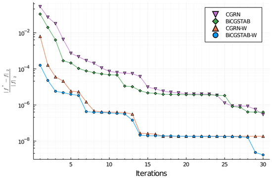
Figure 1.
Relative error for the different conjugate gradients algorithms used, with and without the preconditioner weight matrix , measured as the relative L2 error obtained in the process of direct and inverse Fourier transformation of the initial state input for the 1D Raman case.
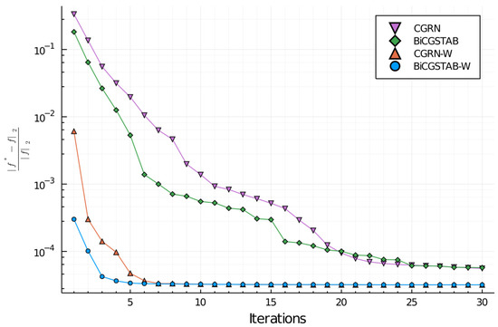
Figure 2.
Relative error for the two different conjugate gradients algorithms used, with and without the preconditioner weight matrix , measured as the relative L2 error obtained in the process of direct and inverse Fourier transformation of the initial state input for the BEC asymmetric case. The Delaunay triangulation is the weight generator for .
It is clear that the FINUFFT algorithm would require more computational cost to reach the solution of a system than the FFT case, but the importance of our work is that there are problems that, by their own nature, cannot be solved with a uniform grid and the use of a non-uniform one is mandatory. Furthermore, the determination and use of the preconditioning matrices allows us to achieve good precision values in relatively few iterations. This is evident in the results section where the values obtained are in good agreement with what was expected.
2.2. The Preconditioning Matrix
To make the convergence of the CG algorithm faster and stable, it is common to incorporate a real diagonal weight matrix as preconditioner, applying as similar to a diagonal matrix as possible; compensating for the clustering effect that could appear during the wavelet filter process that we will explain, later on, at the end of this section.
It is important to note that is not in general an Hermitian matrix, which must be taken into account to solve the linear system via numerical methods. To overcome this problem, we solved the following equivalent preconditioned system:
where is the conjugate transpose matrix of , i.e., the type 1 matrix, and is the aforementioned preconditioning diagonal real matrix.
To determine the elements of the matrix, we could use any quadrature scheme, but we will use the trapezoidal quadrature weights in 1D and a Delaunay triangulation in 2D, where the grid nodes obtained in the filtering process are used as the seeds of the partition.
In this way, in the 1D case, the weight associated to a node is:
However, in the bidimensional case, it is not simple to choose a quadrature scheme which works with any set of scattered points in the plane. To overcome this issue, we have inspired ourselves in a Delaunay triangulated 2D domain.
We can think about a quadrature scheme that approximates the integral of a function over a Delaunay triangle , as the area of the triangle multiplied by the mean value of the function evaluated at the triangle vertices. In this sense, it is direct to obtain that the weight associated to a node is one-third of the sum of the areas of the triangles it belongs to:
we compute the areas using Heron’s formula, which allows us to calculate the area of a triangle knowing the lengths of its sides.
The results for the 1D and 2D cases can be seen in Figure 1 and Figure 2, respectively; the impact of the preconditioning matrix in the convergence of the process is clear, we can achieve in few iterations a low level of error, comparing to the case without preconditioning matrix, which allows us the resolution of the problems proposed with good accuracy and lesser computational effort, thus reducing the total simulation time. More concretely, with the preconditioning matrix, we can achieve the same accuracy that we can without it in a quarter of the simulations or gain one order of magnitude with half the simulations.
Although this work limits itself to 1D and 2D cases, the generalization of (6) to higher dimensions could be achieved in 3D constructing a tetrahedralization of the domain.
2.3. Wavelet Grid Generation and Evolution
To generate the non-uniform grid, we will use the Discrete Wavelet Transform (DWT) that can be viewed, analogously to the FFT, as a matrix linear operator that transforms the power of two length vectors in vectors of the same length but numerically different and is the basis for the wavelet filter process [25].
The effect of the DWT matrix over a column vector looks like the application of two different filters that corresponds to the odd and even rows in the DWT matrix [26]. The odd rows generate a convolution with the data, which, due to the characteristics of the coefficient set, performs some kind of a moving average, a smoothing filter. On the other hand, the even rows, due to a different combination of signs, for the same values of the coefficients, have an opposite effect; in fact, this combination of coefficients is designed to generate a response near to zero as possible for a smooth data vector, performing. therefore, like a detail filter. In our work, we will use the Daubechies wavelets [21], particularly, the set of coefficients DAUB4.
The process to generate the non-homogeneous grid starts with the application of the detail filter; this operation highlights the changes that can appear in the different parts of the data. The value obtained with this operation, if exceeding a previously determined threshold, allows us to adapt the spacing between the nodes of the grid [22], selecting the areas that overcome the threshold and deleting the others. In this way, the filter is applied consecutively to different uniform grids, each of which has twice the point density of the previous one, these uniform grid parts define the layers of our initial non-homogeneous grid as can be seen in Figure 3.
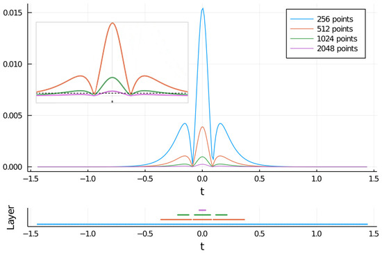
Figure 3.
Results obtained after filtering a order two solitonic pulse, , using the wavelet filter (DAUB4, threshold = 0.0002), details in Appendix B. The values have a similar appearance for the different homogeneous grids (right up inset), their size is inversely proportional to the density of each one of them.The selected coordinates are those for which the result of applying the filter is above the dotted line (left up inset). The selection for every layer is shown on the bottom. The less dense grid is the basis to build the interpolation process when the pulse evolves.
Finally, as we are interested in the evolution of our model, we must ensure the adaptation of the grid to the changes that may appear. We will use interpolation methods [27,28] to refill the areas with a less dense grid; later on, we will apply again the generation scheme to adapt dynamically the grid to possible location changes in the relevant zones of the problem.
3. Results
In this section, we present the physical equations to simulate, i.e., the NLSE and the GPE together with the results obtained. We will use the NLSE to illustrate the process of the grid formation and its adaptation to the evolution of the problem in 1D and the GPE for a 2D example of our scheme.
3.1. NLSE. 1D Raman Scattering
The NLSE has two main terms, each one of these accounting for the two different physical effects this equation applies for: Group Velocity Dispersion (GVD) and Self-Phase Modulation (SPM) [29,30]. With this example, we want to apply our spectral scheme to a challenging nonlinear problem.
The NLSE has the form:
here, represents the slowly varying envelope of the solution, z is the propagation distance and and are the differential operators for the linear (GVD) and the nonlinear (SPM) parts of the equation, respectively.
The separation between both terms is the basis of the time-splitting spectral methods. We start with the linear operator :
in a dispersive medium, the GVD term is a result of the differences in group velocity in a material with respect to the different frequencies that compound the pulse. For a time-splitting spectral approach, this linear part is resolved in the Fourier space.
The nonlinear operator , related to the SPM
accounts for the variation in the refractive index of the medium due to the Kerr effect. This change produces a phase shift in the pulse, leading to a change of the pulse’s frequency spectrum.
The addition of the Raman term to the NLSE makes the soliton fission process appear, splitting a high-order pulse in his solitonic components [31], therefore, the non-uniform grid must adapt to the pulse breaking and the propagation scheme must be able to address a problem with a strong non-linearity.
The intrapulse Raman scattering can be considered as one of the most important higher-order nonlinear effects in the NLSE [32], which was firstly observed by Mitschke et al. [33]; since then, it has been investigated profusely [34,35].
For the Raman scattering, the term added to the right side of the NLSE is:
the coefficient represents the self-induced Raman effect, which produces a downshift in the central frequency of the pulse. In our propagation scheme, the operator associated with the Raman effect is included within the nonlinear operator . In this case, we use an order-one propagation scheme:
In Figure 4, we can observe the rupture of the grid in different parts, each one of them accompanying the different components in which the soliton breaks [36]. Furthermore, the results obtained in the propagation process are in good agreement with the expected values, so we can conclude that the complete scheme, including the linear operator developed in the previous section, is capable of simulating problems of a certain complexity.
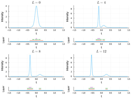
Figure 4.
Intensity plots for different evolution lengths of a order two solitonic pulse input, i.e., ; a Raman term with value has been added to the NLSE in this case. The fission process is clear and in the same way, it is appreciated how the grid is split following each one of the components. Considering a number of 2048 nodes available, base grid of 256 and four layers, the percentage of points used was about 20%.
3.2. GPE. 2D Anisotropic Trap
In some conditions, we can consider the GPE as an NLSE with an extra term accounting for the harmonic trap [37]. In this case, the equation becomes:
where x is the spatial coordinate vector, m is the atomic mass, ℏ is the Planck constant, N is the number of atoms in the condensate, and , and are the trap frequencies in three spatial directions. If all three frequencies are equal, the trap is isotropic. accounts for the interaction between atoms and has the form:
being a the so-called, s-wave scattering length.
In this dimensionless form, according with the notation used in [38] for the 3D case we obtain:
where:
and:
the parameter represents the ratio between the length of the harmonic oscillator ground state in the x-direction () and the characteristic length of the condensate and is the ratio between the trap frequencies.
The other main coefficient in the GPE dimensionless equation is , the nonlinearity coefficient, being:
in our study, we will use, without loss of generality, the dimensionless version of GPE [38] to simulate the BEC.
In this case, we will use the separation of the operators as it appears in the reference [38], in addition, we will take for each step in the evolution of the operators the approach known as Strang splitting that is an order-two algorithm, which is also cited in the previous reference.
In this approach, we have:
where:
and
The temporal steps are resolved using the aforementioned splitting:
From the earliest stages in the BEC research, shape oscillations are a well-known phenomenon both theoretical and experimentally [39,40]. In this example, we will use it to study the feasibility and accuracy of our method in 2D.
In this example, the parameters used to measure the evolution of the solution are: the surface plot of the position density, i.e., and the condensate widths in the different axis.
In the x axis, we have:
with:
brackets denoting space averaging with respect to the position density.
When the value of the parameter is different from 1, the frequencies on the trap are non-degenerate, therefore, we can consider the trap as asymmetric. We will use the 2D approximation with the parameters:
and the initial value:
The results for the position density show consecutive contractions in the axes, as well as a distinct time period for the and widths, in accordance with the experimental observations, these effects are shown in Figure 5. The evolution of the wavelet grid reflects all these differences and is displayed in Figure 6. The concordance of the simulation with the experiment proves the ability of the 2D proposed simulation approach to catch the changes during the evolution of a complex model.
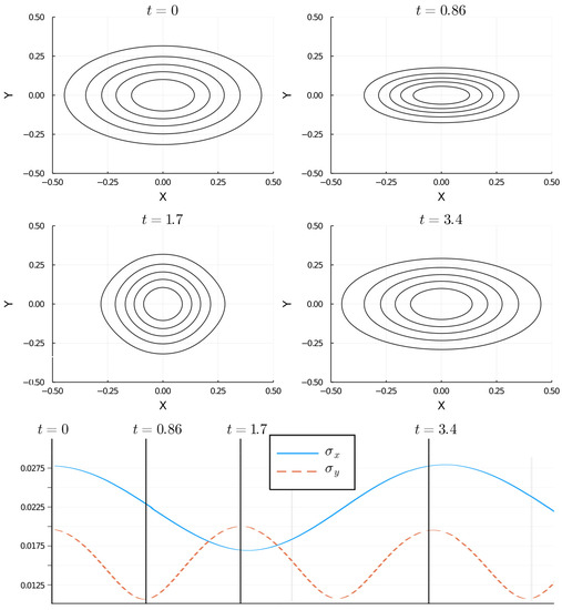
Figure 5.
Contour plot of the position density for the BEC condensate in the asymmetric trap potential with the condition , for different evolution times. In the lower panel, the standard deviation for the same times is shown. In this asymmetric case, the condensate contracts and expands alternately on both axes.
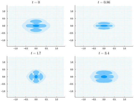
Figure 6.
Evolution of the wavelet-generated grid for the BEC asymmetric case, displaying shape fluctuations according to the position density changes as it is shown in Figure 5. Darker-colored areas indicate denser zones in a four-layer grid. Considering a number of 512 × 512 nodes available, a base grid of 64 × 64 and four layers, the percentage of points used was about 4%.
4. Conclusions
In this work, two conjugate gradient algorithms that allow us the iterative use of the NFFT are developed. A considerable speedup, when a preconditioner matrix is added, can be reached in the calculation of the spectral process. In addition, we show the possibility of using a wavelet filter as generator of a non-homogeneous grid that can be used alongside the aforementioned algorithms to create a solver scheme valid for a wide range of physical problems, obtaining accurate results in 1D and 2D. In particular, the developed preconditioning matrices allow accelerations in the convergence process of two orders of magnitude in the error obtained for the same iterations number.
In this way, this study could be a valid approach for solving problems where the data do not appear homogeneously, e.g., astronomical data series, medical imaging, etc., and it is also applicable to problems with an initial homogeneous mesh that can be adapted using wavelet filters in order to reduce the number of nodes without loss of accuracy.
In future studies, we consider that it could be appropriate to extend the proposed scheme to Graphic Processor Units (GPU) platforms, finally, a generalization to three dimensions, for the case of a rotating dipolar BEC, is beginning to be tested.
Author Contributions
P.R. and M.R. designed the simulations; A.O.-M. and A.M.D.-S. developed the theoretical part. All authors contributed to the analysis and writing of the results of the work. All authors have read and agreed to the published version of the manuscript.
Funding
This research received no external funding. We would like to thank the SICOMFI-TIC176 group of the Physics Department of the University of Córdoba for their support during the researching process.
Data Availability Statement
We are considering the possibility of creating a git-hub type repository with the developed material. On the other hand, we are willing to supply any part of our work to whoever requests it.
Acknowledgments
The authors appreciate the support of C. Quesada Padilla with the grammatical corrections of the final document.
Conflicts of Interest
The authors declare no conflict of interest.
Abbreviations
The following abbreviations are used in this manuscript:
| FFT | Fast Fourier Transform |
| NFFT | Non-uniform Fast Fourier Transform |
| CG | Conjugate Gradient |
| GPE | Gross–Pitaevskii Equation |
| NLSE | Nonlinear Schrodinger Equation |
| GVD | Group Velocity Dispersion |
| SPM | Self-Phase Modulation |
| BEC | Bose Einstein Condensate |
| GPU | Graphic Processor Units |
Appendix A. Conjugate Gradient Algorithms
As is well known, the conjugate gradient method is based on iterative procedures to decrease, in a generic way, the vector of residues. In this work, the two algorithms used have been the Conjugate Gradient for the Normal Equations Residue Normalization (CGNR) [16] and the Preconditioned Biconjugate Gradient Stabilized Method (BiCGSTAB) [17]. The generalities of the method can be found in the reference [16] and the algorithm BiCGSTAB, also used here, are particular realization of it.
| Algorithm A1: Preconditioned conjugate gradients for the normal equations, Residual minimisation (CGNR) |
 |
| Algorithm A2: Preconditioned biconjugate gradient stabilized method (BiCGSTAB) |
 |
Appendix B. Wavelet Grid Generation
As it has been explained in Section 2, the generation of the non-homogeneous grid is one of the main parts of our work. In this appendix we want to explain in more detail how this process is carried out.
In the reference [22] the use of wavelet filters as grid generators is proposed. The algorithm is based on the refinement of a homogeneous base with a thicker separation on which the combination that highlights the details of the data vector is applied by zones. In our case, the set of coefficients used is DAUB4, therefore the application area has a size of four grid points.
The well-known DAUB4 coefficients are:
In this case, the combination of coefficients in a zone of the data vector [25]:
results in a response close to zero for a smooth data vector. The inset in the up-left corner of the Figure 3 show the results for the different grids used and the dotted line the threshold value.
Therefore, by setting a certain threshold we select those positions of the grid where the most relevant changes occur, i.e., those that overcome the threshold value, and we will proceed to place an intermediate point in the center of the segment. In this way, we will have modified the base grid by adding points that belong to a grid twice as dense. The process continues with the newly formed grid. The number of times this algorithm is carried out is set by the number of refinements as it is shown in Figure A1.

Figure A1.
In this figure we can see the flow diagram corresponding to the generation of the non-homogeneous grid. The application of the filter to the different areas of the homogeneous grid produces areas of greater or lesser density.
Figure A1.
In this figure we can see the flow diagram corresponding to the generation of the non-homogeneous grid. The application of the filter to the different areas of the homogeneous grid produces areas of greater or lesser density.

References
- Boyd, W. Nonlinear Optics, 3rd ed.; Elsevier: Amsterdam, The Netherlands, 2008. [Google Scholar]
- Pethick, A.; Smith, H. Bose-Einstein Condensation in Dilute Gases; Cambridge University Press: Cambridge, UK, 2008. [Google Scholar]
- Taha, T.R.; Ablowitz, M.I. Analytical and numerical aspects of certain nonlinear equations: II Nonlinear Schrodinger Equation. J. Comput. Phys. 1984, 55, 203–230. [Google Scholar] [CrossRef]
- Yoshida, H. Construction of higher order symplectic integrators. Phys. Lett. A 1990, 150, 262–268. [Google Scholar] [CrossRef]
- Cooley, J.; Tukey, J. An algorithm for the machine calculation of complex Fourier series. Math. Comput. 1965, 19, 297–301. [Google Scholar] [CrossRef]
- Frigo, M.; Johnson, S.G. The design and implementation of FFTW3. Proc. IEEE 2005, 93, 216–231. [Google Scholar] [CrossRef]
- Fourmont, K. Non-Equispaced Fast Fourier Transforms with Applications to Tomography. J. Fourier Anal. Appl. 2003, 9, 431–450. [Google Scholar] [CrossRef]
- Chan, K.; Tang, S. High-speed spectral domain optical coherence tomography using non-uniform fast Fourier transform. Biomed. Opt. Express 2010, 5, 1309–1319. [Google Scholar] [CrossRef]
- Pelt, J. Fast Computation of Trigonometric Sums with Applications to the Frequency Analysis of Astronomical Data. In Astronomical Time Series; Maoz, D., Sternberg, A., Leibowitz, E.M., Eds.; Astrophysics and Space Science Library; Springer: Dordrecht, Germany, 1997; Volume 218. [Google Scholar]
- Leroy, B. Fast Calculation of the Lomb-Scargle Periodogram using Nonequispaced Fast Fourier Transforms. Astron. Astrophys. 2012, 545, A50. [Google Scholar] [CrossRef]
- Dutt, A.; Rokhlin, V. Fast Fourier Transforms for Nonequiespaced Data II. Appl. Comput. Harmon. Anal. 1995, 2, 85–100. [Google Scholar] [CrossRef]
- Beylkin, G. On the Fast Fourier Transform of Functions with Singularities. Appl. Comput. Harmon. Anal. 1995, 2, 363–381. [Google Scholar] [CrossRef]
- Steidl, G. A Note on Fast Fourier Transforms for Nonequispaced Grids. Adv. Comput. Mech. 1998, 9, 337–352. [Google Scholar]
- Potts, D.; Steidl, G.; Tasche, M. Fast Fourier transforms for nonequispaced data: A tutorial. In Modern Sampling Theory: Mathematics and Applications; Benedetto, J.J., Ferreira, P., Eds.; Springe: Berlin/Heidelberg, Germany, 2001; Chapter 12; pp. 249–274. [Google Scholar]
- Bao, W.; Jiang, S.; Tang, Q.; Zhang, Y. Computing the ground state and dynamics of the nonlinear Schrödinger equation with nonlocal interactions via the nonuniform FFT. J. Comp. Phys. 2015, 296, 72–89. [Google Scholar] [CrossRef]
- Shewchuck, J.R. An Introduction to the Conjugate Gradient Method Without the Agonizing Pain; Carnegie Mellon University: Pittsburgh, PA, USA, 1994. [Google Scholar]
- Gutnechk, M. Variants of BICGSTAB for Matrices with Complex Spectrum. SIAM J. Sci. Comput. 1993, 14, 5. [Google Scholar]
- Barnett, A.H.; Magland, J.F.; Klinteberg, L. A parallel non-uniform fast Fourier transform library based on an “exponential of semicircle’’ kernel. SIAM J. Sci. Comput. 2019, 41, C479–C504. [Google Scholar] [CrossRef]
- Barnett, A.H. Aliasing error of the exp(β1-z2) kernel in the nonuniform fast Fourier transform. Appl. Comput. Harmon. Anal. 2020, 51, 1–16. [Google Scholar] [CrossRef]
- Shih, Y.; Wright, G.; Anden, J.; Blaschke, J.; Barnett, A.H. cuFINUFFT: A load-balanced GPU library for general purpose nonuniform FFTs. In Proceedings of the IEEE International Parallel and Distributed Procesing Symposium Workshops, Portland, OR, USA, 17–21 June 2021. [Google Scholar]
- Daubechies, I. Ten Lectures on Wavelets; SIAM: Philadelphia, PA, USA, 1992. [Google Scholar]
- Jameson, L. Wavelet-Based Grid Generation ICASE Report No. 96-59; Institute for Computer Applications in Science and Engineering: Hampton, VA, USA, 1996. [Google Scholar]
- Greengard, L.; Lee, J.-Y. Accelerating the Nonuniform Fast Fourier Transform. SIAM Rev. 2004, 46, 443. [Google Scholar] [CrossRef]
- Keiner, J.; Kunis, S.; Potts, D. Using NFFT 3—A software library for various nonequispaced fast Fourier transforms. ACM Trans. Math. Softw. 2009, 36, 19. [Google Scholar] [CrossRef]
- Press, W.H.; Teukolsky, S.A.; Vetterling, W.T.; Flannery, B.P. Numerical Recipes: The Art of Scientific Computing, 3rd ed.; Cambridge University Press: Cambridge, UK, 2007. [Google Scholar]
- Vaidyanathan, P.P. Multirate digital filters, filter banks, polyphase networks, and applications: A tutorial. Proc. IEEE 1990, 78, 56–93. [Google Scholar] [CrossRef]
- Harten, A. Adaptative Multiresolution Schemes for Shock Computations. J. Comput. Phys. 1994, 115, 319–328. [Google Scholar] [CrossRef]
- Paolucci, S.; Zikorski, Z.I.; Wirasaet, D. WAMR: An adaptative wavelet method for the simulation of comprensible reacting flow. Part I: Accuraccy and eficciency of algorithm. J. Comput. Phys. 2014, 272, 814–841. [Google Scholar] [CrossRef]
- Akhmediev, N.N.; Ankiewicz, A. Solitons Around Us: Integrable, Hamiltonian and Dissipative Systems. In Optical Solitons; Porsezian, K., Kuriakose, V.C., Eds.; Lecture Notes in Physics; Springer: Berlin/Heidelberg, Germany, 2002; Volume 613. [Google Scholar]
- Agrawall, G. (Ed.) Nonlinear Fiber Optics, 5th ed.; Academic Press: Cambridge, MA, USA, 2013. [Google Scholar]
- Hasegawa, A.; Matsumoto, M. (Eds.) Optical Solitons in Fibers, 3rd ed.; Springer: Berlin/Heidelberg, Germany, 2003. [Google Scholar]
- Gordon, J.P. Theory of the soliton self-frequency shift. Opt. Lett. 1986, 11, 662–664. [Google Scholar] [CrossRef]
- Mitschke, F.; Mollenauer, L.F. Discovery of the soliton self-frequency shift. Opt. Lett. 1986, 11, 659–661. [Google Scholar] [CrossRef] [PubMed]
- Mamyshev, P.V.; Chernikov, S.V. Ultrashort pulse propagation in optical fibers. Opt. Lett. 1990, 15, 1076–1078. [Google Scholar] [CrossRef] [PubMed]
- Stolen, R.H.; Tomlinson, W.J. Effect of the Raman part of the nonlinear refractive index on propagation of ultrashort optical pulses in fibers. J. Opt. Soc. Am. B 1992, 9, 565–573. [Google Scholar] [CrossRef]
- Tai, K.; Hasegawa, A.; Bekki, N. Fission of optical solitons induced by stimulated Raman effect. Opt. Lett. 1988, 13, 392–394. [Google Scholar] [CrossRef] [PubMed]
- Dalfovo, F.; Giorgini, S.; Pitaevskii, L.P.; Stringari, S. Theory of Bose-Einstein condensation in trapped gases. Rev. Mod. Phys. 1999, 71, 463–512. [Google Scholar] [CrossRef]
- Bao, W.; Jaksch, D.; Marcowich, P. Numerical Solution of the Gross-Pitaevskii Equation for Bose-Einstein Condensation. J. Comput. Phys. 2003, 187, 318–342. [Google Scholar] [CrossRef]
- Mewes, M.O.; Andrews, M.R.; van Druten, N.J.; Kurn, D.M.; Durfee, D.S.; Townsend, C.G.; Ketterle, W. Collective Excitations of a Bose-Einstein Condensate in a Magnetic Trap. Phys. Rev. Lett. 1996, 77, 6. [Google Scholar] [CrossRef]
- Stamper-Kurn, D.M.; Andrews, M.R.; Chikkatur, A.P.; Inouye, S.; Miesner, H.-J.; Stenger, J.; Ketterle, W. Optical Confinement of a Bose-Einstein Condensate. Phys. Rev. Lett. 1998, 80, 2027. [Google Scholar] [CrossRef]


Disclaimer/Publisher’s Note: The statements, opinions and data contained in all publications are solely those of the individual author(s) and contributor(s) and not of MDPI and/or the editor(s). MDPI and/or the editor(s) disclaim responsibility for any injury to people or property resulting from any ideas, methods, instructions or products referred to in the content. |
© 2022 by the authors. Licensee MDPI, Basel, Switzerland. This article is an open access article distributed under the terms and conditions of the Creative Commons Attribution (CC BY) license (https://creativecommons.org/licenses/by/4.0/).