Exact Solutions of M-Fractional Kuralay Equation via Three Analytical Schemes

Abstract

This article concerns new analytical wave solutions of the Kuralay-II equations (K-IIAE and K-IIBE) with exploration of a new definition of the derivative. This model is used in various fields, like nonlinear optics, ferromagnetic materials and optical fibers. For this purpose, the ${exp}_a$ function, the extended sinh-Gordon equation expansion scheme, and the generalized Kudryashov schemes were utilized. The resulting solutions are dark, bright, dark-bright, periodic, singular and other kinds of solitons. These results are obtained and also verified by the Mathematica tool. Some of the solutions are explained with 2-D, 3-D and contour plots using the Mathematica tool. The solutions obtained succede the present solutions in the literature. For the first time, the effect of the fractional derivative on the solutions is also shown graphically for this model. The analytical wave solutions are highly desirable as they offer insights into the underlying physics or mathematics of a system and provide a framework for further analysis. The results obtained can also be fruitful for the development of models in the future. The schemes used in this research are effective, easy to apply, and reliably handle other fractional non-linear partial differential equations.

1. Introduction

Fractional partial differential equations (FPDEs) play an important role in many areas, including biology, applied physics, chemistry, economics, etc. Naturally occurring phenomena can be represented in the form of non-linear PDEs, i.e., the extended Zakharov–Kuzetsov equation [1], the fifth order Lax equation [2], the Fokas equation [3], the Clannish Random Walker’s Parabolic equation [4], the Oskolkov equation [5], the Schrödinger dynamical system [6], the generalized unstable Schrödinger equation [7], the generalized Kadomtsev–Petviashvili modified equal-width dynamical equation [8], the dispersive long-wave equation [9], etc. There are many different schemes used to find the distinct types of exact solitons, including the improved generalized Riccati equation mapping method [10], Lie symmetry analysis [11], the generalized Jacobi elliptic function method [12], the exp-function method [13], the Khater method [14], the new modified simplest equation method [15], the new mapping method [16], the extended simplest equation method [17], the first integral method [18], the $(\psi -\varphi )$-expansion method [19], etc.

Three further simple, straightforward and reliable schemes are the ${exp}_a$ function scheme, the extended sinh-Gordon equation expansion scheme, and the generalized Kudryashov scheme. The general ${exp}_a$ function scheme was first proposed by Ahmed T. Ali and Ezzat R. Hassan in 2010 [20]. C. Yan first proposed the extended sinh-Gordon equation expansion method in 1996 [21]. Nikolay A. Kudryashov proposed the generalized Kudryashov scheme. These are three different techniques used for solving nonlinear partial differential equations. These methods seek to determine the vast categories of exact wave solutions. These schemes have many applications that are reported in the literature, including new optical soliton solutions of two nonlinear Schrödinger equations which are obtained by utilizing the ${exp}_a$ function scheme [22]. New kinds of analytical wave solutions of three coupled nonlinear Maccari’s system were obtained by the use of the extended sinh-Gordon equation expansion scheme [23]. Similarly, different types of exact soliton solutions of the fractional Sharma–Tasso–Olver (STO) equation and the fractional Bogoyavlenskii’s breaking soliton equations were found using a generalized Kudryashov method in [24], optical and other types of solitons for different partial differential equations were obtained using this method in [25], some new kinds of exact wave solutions of the Burgers-type fractional space-time differential equations were calculated with the use of a generalized Kudryashov technique in [26], the bell, anti-bell, dark, kink, flat kink and other wave solutions of Fokas–Lenelles were obtained by applying a generalized Kudryashov technique in [27], and exact solitons of the Kudryashov–Burger model were obtained in [28].

Our study model is the M-fractional Kuralay-II equation. This model is used to obtain the gauge equivalence between different models. There are two forms of this equation: the Kuralay-IIA equation (K-IIAE) and the Kuralay-IIB equation (K-IIBE). Different kinds of study of this model are reported in the literature. The simplest soliton solutions of this model were obtained by utilizing the Hirota bilinear scheme [29]. Analytical solitary wave solutions were obtained by applying the new auxiliary equation method [30]. Optical solitons were obtained by utilizing a modified F-expansion and the new extended auxiliary equation methods in [31], etc.

The fundamental purpose of this work is to explore new analytical wave solutions to the space-time fractional Kuralay-II equations (K-IIAE and K-IIBE) with a truncated M-fractional derivative based on the ${exp}_a$ function, the extended sinh-Gordon equation expansion, and the generalized Kudryashov schemes.

The motivation of this paper is to explain the effect of the M-fractional derivative on the solutions of the space-time fractional Kuralay-IIA equation (K-IIAE) and the Kuralay-IIB equation (K-IIBE) that are obtained with the use of the ${exp}_a$ function, the extended sinh-Gordon equation expansion, and the generalized Kudryashov schemes, and this is achieved for the first time in the literature. The significance of the M-fractional derivative is that it fulfils the properties of both integer- and fractional-order derivatives. The fractional- or non-integer-order calculus adds information to the classical calculus, providing a more accurate description of certain natural phenomena. It can be applied in several areas of knowledge, such as physics, chemistry, engineering technology, etc. It is observed that mathematical models obtained by using various fractional derivatives show better overlapping with experimental data. For the truncated M-fractional derivative, the lower fractional orders show the magnitude of the truncated M-fractional derivative to be greater, whereas, for increasing fractional orders, the magnitude remains the same. Fractional differential models successfully explain memory and hereditary effects. By using the extended sinh-Gordon equation expansion scheme, we can obtain the sech, csch, tanh and coth functions involving the solutions. Using these schemes, we can observe some elementary relationships between FNLPDEs and other simple NLODEs. It has been found that, with the use of simple schemes and solvable ODEs, different type of exact solutions of some complicated FNLPDEs can be easily obtained. The solutions obtained supercede the existing solutions in the literature. This model is used in various fields, like nonlinear optics, ferromagnetic materials and optical fibers. Soliton solutions have many advantages: i. the quality of the soliton wave is more efficient as it does not breakup, spread out or become weak over long distances; ii. dispersions are reduced; iii. the speed of transmission over long distances can be increased; iv. it creates the potential for ultrahigh speed highways that are very cost efficient.

The paper is organized as follows: In Section 2, we briefly review some well-known results for the Kuralay-II equations. Some definitions and properties of the M-fractional derivative are presented in Section 3. A description of the methodologies is given in Section 4. Next, in Section 5, we discuss the model description. In Section 6, the mathematical treatment of the model is considered. In Section 7, the analytical wave solutions of K-IIAE are presented. Some analytical wave solutions of K-IIBE are given in Section 8. In Section 9, we explain some solutions graphically. We present the conclusions in the last Section 10.

2. Classical Kuralay-II Equations

In this section, we briefly review the classical Kuralay-II equations. As we mentioned in the Introduction, there are two forms of the Kuralay-II equation: the Kuralay-IIA equation (K-IIAE) and the Kuralay-IIB equation (K-IIBE).

2.1. Kuralay-IIA Equation

The Kuralay-IIA equation (K-IIAE) has the form

$$\begin{array}{c}\hfill i{q}_t+k{q}_{xt}-vq=0,\end{array}$$

(1)

$$\begin{array}{c}\hfill i{r}_t-k{r}_{xt}+vr=0,\end{array}$$

(2)

$$\begin{array}{c}\hfill v_x-2k{\left(rq\right)}_t=0,\end{array}$$

(3)

where $q,r$ are complex functions, v is a real function, and k is some constant. This K-IIAE is integrable. The corresponding Lax representation reads as

$$\begin{array}{c}\hfill {\Phi }_x=U_1\Phi ,\end{array}$$

(4)

$$\begin{array}{c}\hfill {\Phi }_t=V_1\Phi ,\end{array}$$

(5)

where

$$\begin{array}{c}\hfill U_1=-i\lambda {\sigma }_3+Q,\end{array}$$

(6)

$$\begin{array}{c}\hfill V_1=\frac{1}{1-2k\lambda }B,\end{array}$$

(7)

Here

$${\sigma }_3=\left(\begin{array}{cc}1& 0\\ 0& -1\end{array}\right),Q=\left(\begin{array}{cc}0& q\\ r& 0\end{array}\right),B=-0.5iv{\sigma }_3+ik{\sigma }_3{Q}_t.$$

(8)

Hence, the compatibility condition

$$U_{1t}-V_{1x}+[U_1,V_1]=0.$$

(9)

is equivalent to the K-IIAE. Note that there are two particular cases: $k=1$ and $k=i$.

• Case $k=1$

In the case $k=1$, the K-IIAE takes the form

$$\begin{array}{c}\hfill i{q}_t+q_{xt}-vq=0,\end{array}$$

(10)

$$\begin{array}{c}\hfill i{r}_t-r_{xt}+vr=0,\end{array}$$

(11)

$$\begin{array}{c}\hfill v_x-2{\left(rq\right)}_t=0,\end{array}$$

(12)

where $r=ϵ\overline{q},ϵ=\pm 1$. While $\overline{q}$ is the complex conjugate of q. Let us now consider the case $k=i$. In this case, the K-IIAE reads as

$$\begin{array}{c}\hfill q_t+q_{xt}+ivq=0,\end{array}$$

(13)

$$\begin{array}{c}\hfill r_t-r_{xt}-ivr=0,\end{array}$$

(14)

$$\begin{array}{c}\hfill v_x-2i{\left(rq\right)}_t=0,\end{array}$$

(15)

or

$$\begin{array}{c}\hfill q_t+q_{xt}-wq=0,\end{array}$$

(16)

$$\begin{array}{c}\hfill r_t-r_{xt}+wr=0,\end{array}$$

(17)

$$\begin{array}{c}\hfill w_x-2{\left(rq\right)}_t=0,\end{array}$$

(18)

where $w=-iv$ and $r=ϵ\overline{q}$ or $r=ϵq$ with $ϵ=\pm 1$.

2.2. Kuralay-IIB Equation

The Kuralay-IIB equation (K-IIBE) has the form

$$\begin{array}{c}\hfill i{q}_x+k{q}_{xt}-vq=0,\end{array}$$

(19)

$$\begin{array}{c}\hfill i{r}_x-k{r}_{xt}+vr=0,\end{array}$$

(20)

$$\begin{array}{c}\hfill v_t-2k{\left(rq\right)}_x=0,\end{array}$$

(21)

where $q,r$ are complex functions, v is a real function, and k is some constant. This K-IIBE is integrable as is the previous K-IIAE. The Lax representation of the K-IIBE looks like

$$\begin{array}{c}\hfill {\Phi }_t=U_2\Phi ,\end{array}$$

(22)

$$\begin{array}{c}\hfill {\Phi }_x=V_2\Phi ,\end{array}$$

(23)

where

$$\begin{array}{c}\hfill U_2=-i\lambda {\sigma }_3+Q,\end{array}$$

(24)

$$\begin{array}{c}\hfill V_2=\frac{1}{1-2k\lambda }B,\end{array}$$

(25)

Here,

$${\sigma }_3=\left(\begin{array}{cc}1& 0\\ 0& -1\end{array}\right),Q=\left(\begin{array}{cc}0& q\\ r& 0\end{array}\right),B=-0.5iv{\sigma }_3+ik{\sigma }_3{Q}_t.$$

(26)

The compatibility condition

$$U_{2x}-V_{2t}+[U_2,V_2]=0.$$

(27)

gives the K-IIBE. As for the K-IIAE, the K-IIBE admits two particular cases: $k=1$ and $k=i$.

2.2.1. Case $k=1$

In the case $k=1$, the K-IIBE takes the form

$$\begin{array}{c}\hfill i{q}_x+q_{xt}-vq=0,\end{array}$$

(28)

$$\begin{array}{c}\hfill i{r}_x-r_{xt}+vr=0,\end{array}$$

(29)

$$\begin{array}{c}\hfill v_t-2{\left(rq\right)}_x=0,\end{array}$$

(30)

where $r=ϵ\overline{q},ϵ=\pm 1$.

2.2.2. Case $k=i$

Consider the case $k=i$. In this case, the K-IIBE is given by

$$\begin{array}{c}\hfill q_x+q_{xt}+ivq=0,\end{array}$$

(31)

$$\begin{array}{c}\hfill r_x-r_{xt}-ivr=0,\end{array}$$

(32)

$$\begin{array}{c}\hfill v_t-2i{\left(rq\right)}_x=0,\end{array}$$

(33)

or

$$\begin{array}{c}\hfill q_x+q_{xt}-wq=0,\end{array}$$

(34)

$$\begin{array}{c}\hfill r_x-r_{xt}+wr=0,\end{array}$$

(35)

$$\begin{array}{c}\hfill w_t-2{\left(rq\right)}_x=0,\end{array}$$

(36)

where $w=-iv$. In this case, we have two different models: $r=ϵ\overline{q}$ or $r=ϵq$. For convenience, let us present these models.

(a) Case $r=ϵ\overline{q}$. In this instance, the K-IIBE reads as

$$\begin{array}{c}\hfill q_x+q_{xt}-wq=0,\end{array}$$

(37)

$$\begin{array}{c}\hfill r_x-r_{xt}+wr=0,\end{array}$$

(38)

$$\begin{array}{c}\hfill w_t-{2ϵ\left(\right|q|}^2{)}_x=0,\end{array}$$

(39)

(b) Case $r=ϵq$. In this instance, the K-IIBE looks like

$$\begin{array}{c}\hfill q_x+q_{xt}-wq=0,\end{array}$$

(40)

$$\begin{array}{c}\hfill r_x-r_{xt}+wr=0,\end{array}$$

(41)

$$\begin{array}{c}\hfill w_t-4ϵq{q}_x=0,\end{array}$$

(42)

where $r=ϵq$. Note that, in this last case, the functions q and w are complex and/or real valued functions.

3. Truncated M-Fractional Derivative and Its Properties

In this section, we present the main definitions and some properties of the truncated M-fractional derivative.

Definition 1. 

Let $u\left(\theta \right)$:$[0,\infty )\to \mathbb{R}$, then the truncated M-derivative of u of order α is shown in [32]:

$$D_{M,\theta }^{\alpha ,{\rm Y}}u\left(\theta \right)=\underset{\tau \to 0}{lim}\frac{u\left(\theta E_{{\rm Y}}\left(\tau {\theta }^{1-\alpha }\right)\right)-u\left(\theta \right)}{\tau },0<\alpha \le 1,{\rm Y}>0,$$

(43)

where $E_{{\rm Y}}(.)$ represents the truncated Mittag–Leffler function of one parameter that is given as [33]:

$$E_{{\rm Y}}\left(z\right)=\sum _{j=0}^i\frac{z^j}{\Gamma ({\rm Y}j+1)},{\rm Y}>0andz\in \mathit{C}.$$

(44)

Property 1. 

Consider $\alpha \in (0,1],{\rm Y}>0,r,s\in \Re$, and g, f $\alpha$—to be differentiable at a point $\theta >0$, then, by [32]:

$$D_{M,\theta }^{\alpha ,{\rm Y}}(rg\left(\theta \right)+sf\left(\theta \right))=r{D}_{M,\theta }^{\alpha ,{\rm Y}}g\left(\theta \right)+s{D}_{M,\theta }^{\alpha ,{\rm Y}}f\left(\theta \right).$$

(45)

$$D_{M,\theta }^{\alpha ,{\rm Y}}(g\left(t\right).f\left(\theta \right))=g\left(\theta \right)D_{M,\theta }^{\alpha ,{\rm Y}}f\left(\theta \right)+f\left(\theta \right)D_{M,\theta }^{\alpha ,{\rm Y}}g\left(\theta \right).$$

(46)

$$D_{M,\theta }^{\alpha ,{\rm Y}}\left(\frac{g\left(\theta \right)}{f\left(\theta \right)}\right)=\frac{f\left(\theta \right)D_{M,\theta }^{\alpha ,{\rm Y}}g\left(\theta \right)-g\left(\theta \right)D_{M,\theta }^{\alpha ,{\rm Y}}f\left(\theta \right)}{{\left(f\left(\theta \right)\right)}^2}.$$

(47)

$$D_{M,\theta }^{\alpha ,{\rm Y}}\left(A\right)=0,whereAisaconstant.$$

(48)

$$D_{M,\theta }^{\alpha ,{\rm Y}}g\left(\theta \right)=\frac{{\theta }^{1-\alpha }}{\Gamma (1+{\rm Y})}\frac{dg\left(\theta \right)}{d\theta }.$$

(49)

4. Methodologies

4.1. ${exp}_a$ Function Scheme

Here, we provide a complete account of this scheme.

Assuming the non-linear partial differential equation (PDE);

$$G(q,q^2{q}_t,q_x,q_{tt},q_{xx},q_{xt},\dots )=0.$$

(50)

Equation (50) is transformed in the non-linear partial differential equation:

$$\Lambda (Q,Q^{{}^{\prime }},Q^{{}^{″}},\dots ,)=0.$$

(51)

By using the following transformations:

$$q(x,y,t)=Q\left(\zeta \right),\zeta =ax+rt.$$

(52)

where a and r are the parameters.

Considering the root of Equation (51), which is shown in [34,35]:

$$Q\left(\zeta \right)=\frac{{\alpha }_0+{\alpha }_1{d}^{\zeta }+\cdots +{\alpha }_m{d}^{m\zeta }}{{\beta }_0+{\beta }_1{d}^{\zeta }+\cdots +{\beta }_m{d}^{m\zeta }},d\ne 0,1.$$

(53)

where, ${\alpha }_i$ and ${\beta }_i(0\le i\le m)$ are undetermined. The positive integral value of m is calculated by applying a homogeneous balance technique to Equation (51).

Inserting Equation (53) into Equation (51), gives

$$\wp \left(d^{\zeta }\right)={\mathsf{\ell }}_0+{\mathsf{\ell }}_1{d}^{\zeta }+\cdots +{\mathsf{\ell }}_t{d}^{t\zeta }=0.$$

(54)

Taking ${\mathsf{\ell }}_i(0\le i\le t)$ in Equation (54) to be equal to 0, a set of algebraic equations is obtained, given as

$${\mathsf{\ell }}_i=0,wherei=0,\dots ,t.$$

(55)

By using the roots obtained, we obtain the analytical results for Equation (55).

4.2. Extended Sinh–Gordon Equation Expansion Scheme (EShGEES)

Here, we describe the main steps of this technique:

Step 1:

Let a non-linear partial differential equation be given as:

$$Z(f,D_{M,t}^{\alpha ,{\rm Y}}{f}^2,f^2{f}_x,f_y,f_{yy},f_{xx},f_{xy},f_{xt},\dots )=0,$$

(56)

where $f=f(x,y,t)$ denotes the wave function.

Assuming the travelling wave transformation:

$$f(x,y,t)=F\left(\xi \right),\xi =x-\nu y+\frac{\Gamma (1+{\rm Y})}{\alpha }\left(\kappa t^{\alpha }\right).$$

(57)

where, $\mu$ and $\kappa$ are the nonzero parameters. Inserting Equation (57) into Equation (56), we obtain the nonlinear ODE given as:

$$Z(F\left(\xi \right),F^2\left(\xi \right)F^{{}^{\prime }}\left(\xi \right),F^{{}^{″}}\left(\xi \right),\dots )=0.$$

(58)

Step 2:

Assuming the solution of Equation (59) in the given form:

$$F\left(p\right)={\alpha }_0+\sum _{i=1}^m{({\beta }_{i}sinh\left(p\right)+{\alpha }_{i}cosh\left(p\right))}^i,$$

(59)

where, ${\alpha }_0$, ${\alpha }_i$, ${\beta }_i$$(i=1,2,3,\cdots ,m)$ are unknowns. Consider a function p of $\xi$ that satisfies the given equation:

$$\frac{dp}{d\zeta }=sinh\left(p\right).$$

(60)

The natural number m can be obtained by the use of a homogenous balance approach. Equation (58) is derived from the sinh–Gordon equation, shown as:

$$q_{xt}=\kappa sinh\left(v\right).$$

(61)

According to [36], one can gain the solutions of Equation (60) given below:

$$sinhp\left(\xi \right)=\pm csch\left(\xi \right)orcoshp\left(\xi \right)=\pm coth\left(\xi \right),$$

(62)

and

$$sinhp\left(\xi \right)=\pm \iota sech\left(\xi \right)orcoshp\left(\xi \right)=\pm tanh\left(\xi \right),$$

(63)

where ${\iota }^2=-1$.

Step 3:

Applying Equation (59) with Equation (60) to Equation (58), we obtain the algebraic equations involving $p^{{}^{\prime }k}\left(\xi \right){sinh}^{l}p\left(\xi \right){cosh}^{m}p\left(\xi \right)$$(k=0,1;l=0,1;m=0,1,2,\dots )$. Taking every coefficient of $p^{{}^{\prime }k}\left(\zeta \right){sinh}^{l}p\left(\zeta \right){cosh}^{m}p\left(\zeta \right)$ to be equal to 0, to obtain the system of algebraic equations having $\nu ,\kappa ,{\alpha }_0,{\alpha }_i$ and ${\beta }_i(i=1,2,3,\dots ,m)$.

Step 4:

By solving the obtained system of algebraic equations, one may obtain the value of $\nu ,\kappa ,{\alpha }_0,{\alpha }_i$ and ${\beta }_i$.

Step 5:

Using the obtained solutions for Equations (62) and (63), we obtain the wave solitons of Equation (56), shown as:

$$F\left(\xi \right)={\alpha }_0+\sum _{i=1}^m{(\pm {\beta }_{i}csch\left(\xi \right)\pm {\alpha }_{i}coth\left(\xi \right))}^i.$$

(64)

and

$$F\left(\xi \right)={\alpha }_0+\sum _{i=1}^m{(\pm \iota {\beta }_{i}sech\left(\xi \right)\pm {\alpha }_{i}tanh\left(\xi \right))}^i.$$

(65)

4.3. Generalized Kudryashov Scheme

In this part, we briefly describe the basic steps involved in the generalized Kudryashov scheme [25,26]:

Step 1:

Let us assume the non-linear PDE given as:

$$Y(q,q^2{q}_{\gamma },q_{\theta },q_{\theta \theta },q_{\gamma \gamma },q_{\gamma \theta },\dots )=0.$$

(66)

where q is a wave profile and depends on $\gamma$ and $\theta$.

Now, assume the transformations below:

$$q(\gamma ,\theta )=Q\left(\eta \right),\eta =\gamma -\nu \theta .$$

(67)

Here, $\nu$ is a parameter. By inserting Equation (67) into Equation (66), we obtain the following non-linear ODE, as below:

$$F(Q,Q^{{}^{\prime }},Q^2{Q}^{{}^{\prime }},Q^{{}^{″}},Q^2{Q}^{{}^{\prime }},\dots )=0.$$

(68)

where F is the function of Q.

Step 2:

Suppose the solutions of the Equation (68) have the structure:

$$Q\left(\eta \right)={\alpha }_0+\sum _{p=1}^m\frac{{\alpha }_p}{{(1+\psi \left(\eta \right))}^p}.$$

(69)

where ${\alpha }_0$ and ${\alpha }_p$, $(p=1,2,3,\cdots ,m)$ are unknown parameters that are found later and $\psi$ is a new function of $\eta$ that is a solution of the general Riccati equation, given as follow:

$${\psi }^{\prime }\left(\eta \right)=\rho +\sigma \psi \left(\eta \right)+\omega {\psi }^2\left(\eta \right).$$

(70)

where, $\rho$, $\sigma$ and $\omega$ are constants.

The solutions of the Equation (70) are shown for the following cases [37]:

Case 1: If all of $\rho$, $\sigma$ and $\omega$ are nonzero, then $\psi \left(\eta \right)$ is given by

$$\psi \left(\eta \right)=\frac{1}{2\omega }\left(\sqrt{4\rho \omega -{\sigma }^2}tan\left(\frac{1}{2}\sqrt{4\rho \omega -{\sigma }^2}\left(d_0+\eta \right)\right)-\sigma \right),4\rho \omega >{\sigma }^2.$$

(71)

$$\psi \left(\eta \right)=\frac{-1}{2\omega }\left(\sqrt{4\rho \omega -{\sigma }^2}cot\left(\frac{1}{2}\sqrt{4\rho \omega -{\sigma }^2}\left(d_0+\eta \right)\right)+\sigma \right),4\rho \omega >{\sigma }^2.$$

(72)

$$\psi \left(\eta \right)=\frac{-1}{2\omega }\left(\sqrt{4\rho \omega -{\sigma }^2}tanh\left(\frac{1}{2}\sqrt{4\rho \omega -{\sigma }^2}\left(d_0+\eta \right)\right)+\sigma \right),4\rho \omega <{\sigma }^2.$$

(73)

$$\psi \left(\eta \right)=\frac{-1}{2\omega }\left(\sqrt{4\rho \omega -{\sigma }^2}coth\left(\frac{1}{2}\sqrt{4\rho \omega -{\sigma }^2}\left(d_0+\eta \right)\right)+\sigma \right),4\rho \omega <{\sigma }^2.$$

(74)

$$\psi \left(\eta \right)=\frac{-1}{\omega }\left(\frac{1}{d_0+\eta }+\frac{\sigma }{2}\right),4\rho \omega ={\sigma }^2.$$

(75)

Case 2: If $\rho =0$ and $\omega \ne 0$, then

$$\psi \left(\eta \right)=\frac{-1}{2\omega }\left(\sigma tanh\left(\frac{\sigma }{2}\left(d_0+\eta \right)\right)+\sigma \right),{\sigma }^2>0.$$

(76)

$$\psi \left(\eta \right)=\frac{-1}{2\omega }\left(\sigma coth\left(\frac{\sigma }{2}\left(d_0+\eta \right)\right)+\sigma \right),{\sigma }^2>0.$$

(77)

$$\psi \left(\eta \right)=\frac{1}{2\omega }\left(\sqrt{-{\sigma }^2}tan\left(\frac{\sqrt{-{\sigma }^2}}{2}\left(d_0+\eta \right)\right)-\sigma \right),{\sigma }^2<0.$$

(78)

$$\psi \left(\eta \right)=\frac{-1}{2\omega }\left(\sqrt{-{\sigma }^2}cot\left(\frac{\sqrt{-{\sigma }^2}}{2}\left(d_0+\eta \right)\right)+\sigma \right),{\sigma }^2<0.$$

(79)

$$\psi \left(\eta \right)=\frac{\sigma }{\sigma exp(-\sigma (d_0+\eta ))-\omega },\sigma \ne 0.$$

(80)

$$\psi \left(\eta \right)=\frac{-1}{\omega \eta },\sigma =0.$$

(81)

Case 3: If $\sigma =0$ and $\omega \ne 0$, then

$$\psi \left(\eta \right)=\frac{\sqrt{\rho \omega }}{\omega }tan\left(\sqrt{\rho \omega }\left(d_0+\eta \right)\right),\rho \omega >0.$$

(82)

$$\psi \left(\eta \right)=-\frac{\sqrt{\rho \omega }}{\omega }cot\left(\sqrt{\rho \omega }\left(d_0+\eta \right)\right),\rho \omega >0.$$

(83)

$$\psi \left(\eta \right)=-\frac{\sqrt{\rho \omega }}{\omega }tanh\left(\sqrt{-\rho \omega }\left(d_0+\eta \right)\right),\rho \omega <0.$$

(84)

$$\psi \left(\eta \right)=-\frac{\sqrt{\rho \omega }}{\omega }coth\left(\sqrt{-\rho \omega }\left(d_0+\eta \right)\right),\rho \omega <0.$$

(85)

$$\psi \left(\eta \right)=\frac{-1}{\omega (d_0+\eta )},\rho =0.$$

(86)

Case 4: If $\omega =0$ and $\sigma \ne 0$, then

$$\psi \left(\eta \right)=\frac{1}{\sigma }\left(exp\left(\sigma (d_0+\eta )\right)-\rho \right).$$

(87)

Step 3: Inserting Equation (69) into Equation (68) and summing the coefficients of the same power of $\psi \left(\eta \right)$. Now, taking the coefficient of each power equal to zero, we obtain a system of algebraic equations involving ${\alpha }_0$ and ${\alpha }_p$, $(p=1,2,3,\dots ,m)$ and the other parameters. By solving this system with the help of the Mathematica software, we obtain the values of the unknowns.

Step 4: Now, by inserting the values of ${\alpha }_0$ and ${\alpha }_p$, $(p=1,2,3,\dots ,m)$ into Equation (69), and using the suitable cases of the general Riccati equation given from Equations (71)–(87), we obtain the solutions for Equation (66).

5. Model Description

Consider the M-fractional Kuralay-II equation, given as [29]:

$$\iota D_{M,t}^{\alpha ,{\rm Y}}u+D_{M,x}^{\alpha ,{\rm Y}}\left(D_{M,t}^{\alpha ,{\rm Y}}u\right)-vu=0.$$

(88)

$$D_{M,x}^{\alpha ,{\rm Y}}v-2ϵD_{M,t}^{\alpha ,{\rm Y}}{\left|u\right|}^2=0.$$

(89)

where, $u=u(x,t)$ is a complex valued function, while $v=v(x,t)$ is a real valued function. The conjugate of the complex valued function u is $u^{*}$, $ϵ=\pm 1$, where x and t are the spatio-temporal real variables. There are two forms of the Kuralay equation.

5.1. Kuralay-IIA Equation (K-IIAE)

Let us assume the following form of the Kuralay-II equation (K-IIE), given as

$$\iota D_{M,t}^{\alpha ,{\rm Y}}u-D_{M,x}^{\alpha ,{\rm Y}}\left(D_{M,t}^{\alpha ,{\rm Y}}u\right)-vu=0.$$

(90)

$$\iota D_{M,t}^{\alpha ,{\rm Y}}r+D_{M,x}^{\alpha ,{\rm Y}}\left(D_{M,t}^{\alpha ,{\rm Y}}r\right)+vr=0.$$

(91)

$$D_{M,x}^{\alpha ,{\rm Y}}v+2d^2{D}_{M,t}^{\alpha ,{\rm Y}}\left(ru\right)=0.$$

(92)

this is called the K-IIAE. It is integrable.

5.2. Kuralay-IIB Equation (K-IIBE)

Let us assume the second form of the Kuralay-II equation (K-IIE), given as

$$\iota D_{M,t}^{\alpha ,{\rm Y}}u+D_{M,x}^{\alpha ,{\rm Y}}\left(D_{M,t}^{\alpha ,{\rm Y}}u\right)-vu=0.$$

(93)

$$\iota D_{M,t}^{\alpha ,{\rm Y}}r-D_{M,x}^{\alpha ,{\rm Y}}\left(D_{M,t}^{\alpha ,{\rm Y}}r\right)+vr=0.$$

(94)

$$D_{M,t}^{\alpha ,{\rm Y}}v-2D_{M,x}^{\alpha ,{\rm Y}}\left(ru\right)=0.$$

(95)

This is called the K-IIBE. This also integrable.

6. Mathematical Treatment of the Model

6.1. K-IIAE

Consider the truncated M-fractional K-IIA equation for $d=1$, $r=ϵu^{*}$, given as follows:

$$\iota D_{M,t}^{\alpha ,{\rm Y}}u-D_{M,x}^{\alpha ,{\rm Y}}\left(D_{M,t}^{\alpha ,{\rm Y}}u\right)-vu=0.$$

(96)

$$D_{M,x}^{\alpha ,{\rm Y}}v-2ϵD_{M,t}^{\alpha ,{\rm Y}}{\left(\right|u|}^2)=0.$$

(97)

Let us consider the following travelling wave transformations:

$$u(x,t)=U\left(\zeta \right)\times exp\left(\iota \left(\frac{\Gamma (1+{\rm Y})}{\alpha }(\tau x^{\alpha }+\mu t^{\alpha })\right)\right),v(x,t)=v\left(\zeta \right),\zeta =\frac{\Gamma (1+{\rm Y})}{\alpha }(\Omega x^{\alpha }+\lambda t^{\alpha }).$$

(98)

where, $\tau$, $\mu$, $\Omega$ and $\lambda$ are the parameters. By inserting Equation (98) into Equations (96) and (97), we obtain the real and imaginary parts, given as: real part:

$$2\lambda U^3ϵ-U\Omega (\mu (\tau -1)-c)+\lambda {\Omega }^2{U}^{″}=0.$$

(99)

imaginary part:

$$(\lambda -\tau \lambda -\mu \Omega )U^{\prime }=0.$$

(100)

From Equation (100), we obtain the speed of the soliton, given as:

$$\lambda =\frac{\mu \Omega }{1-\tau }.$$

(101)

By using the homogeneous balance technique into Equation (99), we obtain $m=1$.

6.2. K-IIBE

Consider the truncated M-fractional K-IIB equation for $r=ϵu^{*}$, given as:

$$\iota D_{M,t}^{\alpha ,{\rm Y}}u+D_{M,x}^{\alpha ,{\rm Y}}\left(D_{M,t}^{\alpha ,{\rm Y}}u\right)-vu=0.$$

(102)

$$D_{M,t}^{\alpha ,{\rm Y}}v+2ϵD_{M,x}^{\alpha ,{\rm Y}}{\left(\right|u|}^2)=0.$$

(103)

Let us consider the following travelling wave transformations:

$$u(x,t)=U\left(\zeta \right)\times exp\left(\iota \left(\frac{\Gamma (1+{\rm Y})}{\alpha }(\tau x^{\alpha }+\mu t^{\alpha })\right)\right),v(x,t)=v\left(\zeta \right),\zeta =\frac{\Gamma (1+{\rm Y})}{\alpha }(\Omega x^{\alpha }+\lambda t^{\alpha }).$$

(104)

By inserting Equation (104) into Equations (102) and (103), we obtain the real and imaginary parts, given as: real part:

$$2U^3\Omega ϵ-\lambda U(\mu (\tau +1)-c)+{\lambda }^2\Omega U^{″}=0.$$

(105)

imaginary part:

$$(\lambda +\tau \lambda +\mu \Omega )U^{\prime }=0.$$

(106)

From Equation (106), we obtain the speed of the soliton, given as:

$$\lambda =-\frac{\mu \Omega }{1+\tau }.$$

(107)

By inserting the homogeneous balance technique into Equation (105), we obtain $m=1$.

7. Analytical Wave Solutions of K-IIAE

7.1. By ${exp}_a$ Function Scheme

Equation (68) changes into the following for $m=1$:

$$U\left(\zeta \right)=\frac{{\alpha }_0+{\alpha }_1{d}^{\zeta }}{{\beta }_0+{\beta }_1{d}^{\zeta }}.$$

(108)

Inserting Equations (53) into Equation (99), a system of equations is achieved. By solving the system, we obtain different solution sets, given as follows:

Set 1:

$$\left\{{\alpha }_0=-\frac{i{\beta }_0\Omega log\left(d\right)}{2\sqrt{ϵ}},{\alpha }_1=\frac{i{\beta }_1\Omega log\left(d\right)}{2\sqrt{ϵ}},\mu =\frac{2c-\lambda \Omega {log}^2\left(d\right)}{2(\tau -1)}\right\}.$$

(109)

$$u(x,t)=-\frac{i\Omega log\left(d\right)}{2\sqrt{ϵ}}\left(\frac{{\beta }_0-{\beta }_1{d}^{\left(\frac{\Gamma (1+{\rm Y})}{\alpha }(\Omega x^{\alpha }+\left(\frac{\mu \Omega }{1-\tau }\right)t^{\alpha })\right)}}{{\beta }_0+{\beta }_1{d}^{\left(\frac{\Gamma (1+{\rm Y})}{\alpha }(\Omega x^{\alpha }+\left(\frac{\mu \Omega }{1-\tau }\right)t^{\alpha })\right)}}\right)\times exp\left(\iota \left(\frac{\Gamma (1+{\rm Y})}{\alpha }(\tau x^{\alpha }+\mu t^{\alpha })\right)\right).$$

(110)

where $\mu$ is given in Equation (109).

Set 2:

$$\left\{{\alpha }_0=\frac{i{\beta }_0\Omega log\left(d\right)}{2\sqrt{ϵ}},{\alpha }_1=-\frac{i{\beta }_1\Omega log\left(d\right)}{2\sqrt{ϵ}},\mu =\frac{2c-\lambda \Omega {log}^2\left(d\right)}{2(\tau -1)}\right\}.$$

(111)

$$u(x,t)=\frac{i\Omega log\left(d\right)}{2\sqrt{ϵ}}\left(\frac{{\beta }_0-{\beta }_1{d}^{\left(\frac{\Gamma (1+{\rm Y})}{\alpha }(\Omega x^{\alpha }+\left(\frac{\mu \Omega }{1-\tau }\right)t^{\alpha })\right)}}{{\beta }_0+{\beta }_1{d}^{\left(\frac{\Gamma (1+{\rm Y})}{\alpha }(\Omega x^{\alpha }+\left(\frac{\mu \Omega }{1-\tau }\right)t^{\alpha })\right)}}\right)\times exp\left(\iota \left(\frac{\Gamma (1+{\rm Y})}{\alpha }(\tau x^{\alpha }+\mu t^{\alpha })\right)\right).$$

(112)

where $\mu$ is given in Equation (111).

7.2. By the Extended Sinh-Gordon Equation Expansion Scheme

For $m=1$, Equations (59), (62) and (63) become:

$$U\left(\zeta \right)={\alpha }_0\pm {\beta }_{1}csch\left(\zeta \right)\pm {\alpha }_{1}coth\left(\zeta \right).$$

(113)

$$U\left(\zeta \right)={\alpha }_0\pm \iota {\beta }_{1}sech\left(\zeta \right)\pm {\alpha }_{1}tanh\left(\zeta \right).$$

(114)

$$U\left(\zeta \right)={\alpha }_0+{\beta }_{1}sinh\left(p\right)+{\alpha }_{1}cosh\left(p\right).$$

(115)

where, ${\alpha }_0,{\alpha }_1\mathrm{and}{\beta }_1$ are undetermined. Inserting Equation (115) into Equation (99), we obtain algebraic equations containing ${\alpha }_0,{\alpha }_1,{\beta }_1$ and the other parameters. By using the Mathematica tool, we obtain different solution sets, given as:

Set 1:

$$\left\{{\alpha }_0=0,{\alpha }_1=-\frac{i\Omega }{\sqrt{ϵ}},{\beta }_1=0,\mu =\frac{c-2\lambda \Omega }{\tau -1}\right\}.$$

(116)

$$u_1(x,t)=\mp \frac{i\Omega }{\sqrt{ϵ}}coth\left(\frac{\Gamma (1+{\rm Y})}{\alpha }(\Omega x^{\alpha }+\left(\frac{\mu \Omega }{1-\tau }\right)t^{\alpha })\right)\times exp\left(\iota \left(\frac{\Gamma (1+{\rm Y})}{\alpha }(\tau x^{\alpha }+\mu t^{\alpha })\right)\right).$$

(117)

$$u_2(x,t)=\mp \frac{i\Omega }{\sqrt{ϵ}}tanh\left(\frac{\Gamma (1+{\rm Y})}{\alpha }(\Omega x^{\alpha }+\left(\frac{\mu \Omega }{1-\tau }\right)t^{\alpha })\right)\times exp\left(\iota \left(\frac{\Gamma (1+{\rm Y})}{\alpha }(\tau x^{\alpha }+\mu t^{\alpha })\right)\right).$$

(118)

where $\mu$ is given in Equation (116).

Set 2:

$$\left\{{\alpha }_0=0,{\alpha }_1=\frac{i\Omega }{\sqrt{ϵ}},{\beta }_1=0,\mu =\frac{c-2\lambda \Omega }{\tau -1}\right\}.$$

(119)

$$u_1(x,t)=\pm \frac{i\Omega }{\sqrt{ϵ}}coth\left(\frac{\Gamma (1+{\rm Y})}{\alpha }(\Omega x^{\alpha }+\left(\frac{\mu \Omega }{1-\tau }\right)t^{\alpha })\right)\times exp\left(\iota \left(\frac{\Gamma (1+{\rm Y})}{\alpha }(\tau x^{\alpha }+\mu t^{\alpha })\right)\right).$$

(120)

$$u_2(x,t)=\pm \frac{i\Omega }{\sqrt{ϵ}}tanh\left(\frac{\Gamma (1+{\rm Y})}{\alpha }(\Omega x^{\alpha }+\left(\frac{\mu \Omega }{1-\tau }\right)t^{\alpha })\right)\times exp\left(\iota \left(\frac{\Gamma (1+{\rm Y})}{\alpha }(\tau x^{\alpha }+\mu t^{\alpha })\right)\right).$$

(121)

where $\mu$ is given in Equation (119).

Set 3:

$$\left\{{\alpha }_0=0,{\alpha }_1=-\frac{i\Omega }{2\sqrt{ϵ}},{\beta }_1=-\frac{i\Omega }{2\sqrt{ϵ}},\mu =\frac{2c-\lambda \Omega }{2(\tau -1)}\right\}.$$

(122)

$$\begin{array}{c}{u}_1(x,t)=\mp \frac{i\Omega }{2\sqrt{ϵ}}(coth\left(\frac{\Gamma (1+{\rm Y})}{\alpha }(\Omega x^{\alpha }+\left(\frac{\mu \Omega }{1-\tau }\right)t^{\alpha })\right)+\mathrm{csch}\left(\frac{\Gamma (1+{\rm Y})}{\alpha }(\Omega x^{\alpha }+\left(\frac{\mu \Omega }{1-\tau }\right)t^{\alpha })\right))\hfill \\ \hfill \times exp\left(\iota \left(\frac{\Gamma (1+{\rm Y})}{\alpha }(\tau x^{\alpha }+\mu t^{\alpha })\right)\right).\end{array}$$

(123)

$$\begin{array}{c}{u}_2(x,t)=\mp \frac{i\Omega }{2\sqrt{ϵ}}(\iota \mathrm{sech}\left(\frac{\Gamma (1+{\rm Y})}{\alpha }(\Omega x^{\alpha }+\left(\frac{\mu \Omega }{1-\tau }\right)t^{\alpha })\right)+tanh\left(\frac{\Gamma (1+{\rm Y})}{\alpha }(\Omega x^{\alpha }+\left(\frac{\mu \Omega }{1-\tau }\right)t^{\alpha })\right))\hfill \\ \hfill \times exp\left(\iota \left(\frac{\Gamma (1+{\rm Y})}{\alpha }(\tau x^{\alpha }+\mu t^{\alpha })\right)\right).\end{array}$$

(124)

where $\mu$ is given in Equation (122).

Set 4:

$$\left\{{\alpha }_0=0,{\alpha }_1=\frac{i\Omega }{2\sqrt{ϵ}},{\beta }_1=-\frac{i\Omega }{2\sqrt{ϵ}},\mu =\frac{2c-\lambda \Omega }{2(\tau -1)}\right\}.$$

(125)

$$\begin{array}{c}{u}_1(x,t)=\frac{i\Omega }{2\sqrt{ϵ}}(\mp \mathrm{csch}\left(\frac{\Gamma (1+{\rm Y})}{\alpha }(\Omega x^{\alpha }+\left(\frac{\mu \Omega }{1-\tau }\right)t^{\alpha })\right)\pm coth\left(\frac{\Gamma (1+{\rm Y})}{\alpha }(\Omega x^{\alpha }+\left(\frac{\mu \Omega }{1-\tau }\right)t^{\alpha })\right))\hfill \\ \hfill \times exp\left(\iota \left(\frac{\Gamma (1+{\rm Y})}{\alpha }(\tau x^{\alpha }+\mu t^{\alpha })\right)\right).\end{array}$$

(126)

$$\begin{array}{c}{u}_2(x,t)=\frac{i\Omega }{2\sqrt{ϵ}}(\mp \iota \mathrm{sech}\left(\frac{\Gamma (1+{\rm Y})}{\alpha }(\Omega x^{\alpha }+\left(\frac{\mu \Omega }{1-\tau }\right)t^{\alpha })\right)\pm tanh\left(\frac{\Gamma (1+{\rm Y})}{\alpha }(\Omega x^{\alpha }+\left(\frac{\mu \Omega }{1-\tau }\right)t^{\alpha })\right))\hfill \\ \hfill \times exp\left(\iota \left(\frac{\Gamma (1+{\rm Y})}{\alpha }(\tau x^{\alpha }+\mu t^{\alpha })\right)\right).\end{array}$$

(127)

where $\mu$ is given in Equation (125).

Set 5:

$$\left\{{\alpha }_0=0,{\alpha }_1=-\frac{i\Omega }{2\sqrt{ϵ}},{\beta }_1=\frac{i\Omega }{2\sqrt{ϵ}},\mu =\frac{2c-\lambda \Omega }{2(\tau -1)}\right\}.$$

(128)

$$\begin{array}{c}{u}_1(x,t)=\frac{i\Omega }{2\sqrt{ϵ}}(\pm \mathrm{csch}\left(\frac{\Gamma (1+{\rm Y})}{\alpha }(\Omega x^{\alpha }+\left(\frac{\mu \Omega }{1-\tau }\right)t^{\alpha })\right)\mp coth\left(\frac{\Gamma (1+{\rm Y})}{\alpha }(\Omega x^{\alpha }+\left(\frac{\mu \Omega }{1-\tau }\right)t^{\alpha })\right))\hfill \\ \hfill \times exp\left(\iota \left(\frac{\Gamma (1+{\rm Y})}{\alpha }(\tau x^{\alpha }+\mu t^{\alpha })\right)\right).\end{array}$$

(129)

$$\begin{array}{c}{u}_2(x,t)=\frac{i\Omega }{2\sqrt{ϵ}}(\pm \iota \mathrm{sech}\left(\frac{\Gamma (1+{\rm Y})}{\alpha }(\Omega x^{\alpha }+\left(\frac{\mu \Omega }{1-\tau }\right)t^{\alpha })\right)\mp tanh\left(\frac{\Gamma (1+{\rm Y})}{\alpha }(\Omega x^{\alpha }+\left(\frac{\mu \Omega }{1-\tau }\right)t^{\alpha })\right))\hfill \\ \hfill \times exp\left(\iota \left(\frac{\Gamma (1+{\rm Y})}{\alpha }(\tau x^{\alpha }+\mu t^{\alpha })\right)\right).\end{array}$$

(130)

where $\mu$ is given in Equation (128).

Set 6:

$$\left\{{\alpha }_0=0,{\alpha }_1=\frac{i\Omega }{2\sqrt{ϵ}},{\beta }_1=\frac{i\Omega }{2\sqrt{ϵ}},\mu =\frac{2c-\lambda \Omega }{2(\tau -1)}\right\}.$$

(131)

$$\begin{array}{c}{u}_1(x,t)=\pm \frac{i\Omega }{2\sqrt{ϵ}}(coth\left(\frac{\Gamma (1+{\rm Y})}{\alpha }(\Omega x^{\alpha }+\left(\frac{\mu \Omega }{1-\tau }\right)t^{\alpha })\right)+\mathrm{csch}\left(\frac{\Gamma (1+{\rm Y})}{\alpha }(\Omega x^{\alpha }+\left(\frac{\mu \Omega }{1-\tau }\right)t^{\alpha })\right))\hfill \\ \hfill \times exp\left(\iota \left(\frac{\Gamma (1+{\rm Y})}{\alpha }(\tau x^{\alpha }+\mu t^{\alpha })\right)\right).\end{array}$$

(132)

$$\begin{array}{c}{u}_2(x,t)=\pm \frac{i\Omega }{2\sqrt{ϵ}}(\iota \mathrm{sech}\left(\frac{\Gamma (1+{\rm Y})}{\alpha }(\Omega x^{\alpha }+\left(\frac{\mu \Omega }{1-\tau }\right)t^{\alpha })\right)+tanh\left(\frac{\Gamma (1+{\rm Y})}{\alpha }(\Omega x^{\alpha }+\left(\frac{\mu \Omega }{1-\tau }\right)t^{\alpha })\right))\hfill \\ \hfill \times exp\left(\iota \left(\frac{\Gamma (1+{\rm Y})}{\alpha }(\tau x^{\alpha }+\mu t^{\alpha })\right)\right).\end{array}$$

(133)

where $\mu$ is given in Equation (131).

Set 7:

$$\left\{{\alpha }_0=0,{\alpha }_1=0,{\beta }_1=-\frac{i\Omega }{\sqrt{ϵ}},\mu =\frac{c+\lambda \Omega }{\tau -1}\right\}.$$

(134)

$$u_1(x,t)=\mp \frac{i\Omega }{\sqrt{ϵ}}\mathrm{csch}\left(\frac{\Gamma (1+{\rm Y})}{\alpha }(\Omega x^{\alpha }+\left(\frac{\mu \Omega }{1-\tau }\right)t^{\alpha })\right)\times exp\left(\iota \left(\frac{\Gamma (1+{\rm Y})}{\alpha }(\tau x^{\alpha }+\mu t^{\alpha })\right)\right).$$

(135)

$$u_2(x,t)=\pm \frac{\Omega }{\sqrt{ϵ}}\mathrm{sech}\left(\frac{\Gamma (1+{\rm Y})}{\alpha }(\Omega x^{\alpha }+\left(\frac{\mu \Omega }{1-\tau }\right)t^{\alpha })\right)\times exp\left(\iota \left(\frac{\Gamma (1+{\rm Y})}{\alpha }(\tau x^{\alpha }+\mu t^{\alpha })\right)\right).$$

(136)

where $\mu$ is given in Equation (134).

Set 8:

$$\left\{{\alpha }_0=0,{\alpha }_1=0,{\beta }_1=\frac{i\Omega }{\sqrt{ϵ}},\mu =\frac{c+\lambda \Omega }{\tau -1}\right\}.$$

(137)

$$u_1(x,t)=\pm \frac{i\Omega }{\sqrt{ϵ}}\mathrm{csch}\left(\frac{\Gamma (1+{\rm Y})}{\alpha }(\Omega x^{\alpha }+\left(\frac{\mu \Omega }{1-\tau }\right)t^{\alpha })\right)\times exp\left(\iota \left(\frac{\Gamma (1+{\rm Y})}{\alpha }(\tau x^{\alpha }+\mu t^{\alpha })\right)\right).$$

(138)

$$u_2(x,t)=\mp \frac{\Omega }{\sqrt{ϵ}}\mathrm{sech}\left(\frac{\Gamma (1+{\rm Y})}{\alpha }(\Omega x^{\alpha }+\left(\frac{\mu \Omega }{1-\tau }\right)t^{\alpha })\right)\times exp\left(\iota \left(\frac{\Gamma (1+{\rm Y})}{\alpha }(\tau x^{\alpha }+\mu t^{\alpha })\right)\right).$$

(139)

where $\mu$ is given in Equation (137).

7.3. By the Generalized Kudryashov Scheme

For $m=1$, Equation (69) reduces to:

$$U\left(\eta \right)={\alpha }_0+\frac{{\alpha }_1}{1+\psi \left(\eta \right)}.$$

(140)

where, ${\alpha }_0$ and ${\alpha }_1$ are unknown constants. By inserting Equation (140) into Equation (99) with Equation (70) and collecting all the coefficients of the same order of $\psi \left(\eta \right)$, we obtain the algebraic equation involving ${\alpha }_0$, ${\alpha }_1$ and the other parameters. Now, using the Wolfram Mathematica aid, we obtain the solution set below:

Set 1:

$$\left\{{\alpha }_0=-\frac{i\Omega (\sigma -2\omega )}{2\sqrt{ϵ}},{\alpha }_1=-\frac{i\Omega (\rho -\sigma +\omega )}{\sqrt{ϵ}},\mu =\frac{2c-\lambda \Omega \left({\sigma }^2-4\rho \omega \right)}{2(\tau -1)}\right\}.$$

(141)

Case 1:

$$\begin{array}{c}u(x,t)=-\frac{i\Omega }{\sqrt{ϵ}}(\frac{\sigma -2\omega }{2}+\frac{\rho -\sigma +\omega }{1+\left(\frac{1}{2\omega }\left(\sqrt{4\rho \omega -{\sigma }^2}tan\left(\frac{1}{2}\sqrt{4\rho \omega -{\sigma }^2}\left(d_0+\frac{\Gamma (1+{\rm Y})}{\alpha }(\Omega x^{\alpha }+\left(\frac{\mu \Omega }{1-\tau }\right)t^{\alpha })\right)\right)-\sigma \right)\right)})\hfill \\ \hfill \times exp\left(\iota \left(\frac{\Gamma (1+{\rm Y})}{\alpha }(\tau x^{\alpha }+\mu t^{\alpha })\right)\right).\end{array}$$

(142)

$$\begin{array}{c}u(x,t)=-\frac{i\Omega }{\sqrt{ϵ}}(\frac{\sigma -2\omega }{2}+\frac{\rho -\sigma +\omega }{1+\left(\frac{-1}{2\omega }\left(\sqrt{4\rho \omega -{\sigma }^2}cot\left(\frac{1}{2}\sqrt{4\rho \omega -{\sigma }^2}\left(d_0+\frac{\Gamma (1+{\rm Y})}{\alpha }(\Omega x^{\alpha }+\left(\frac{\mu \Omega }{1-\tau }\right)t^{\alpha })\right)\right)+\sigma \right)\right)})\hfill \\ \hfill \times exp\left(\iota \left(\frac{\Gamma (1+{\rm Y})}{\alpha }(\tau x^{\alpha }+\mu t^{\alpha })\right)\right).\end{array}$$

(143)

$$\begin{array}{c}u(x,t)=-\frac{i\Omega }{\sqrt{ϵ}}(\frac{\sigma -2\omega }{2}+\frac{\rho -\sigma +\omega }{1+\left(\frac{-1}{2\omega }\left(\sqrt{4\rho \omega -{\sigma }^2}tanh\left(\frac{1}{2}\sqrt{4\rho \omega -{\sigma }^2}\left(d_0+\frac{\Gamma (1+{\rm Y})}{\alpha }(\Omega x^{\alpha }+\left(\frac{\mu \Omega }{1-\tau }\right)t^{\alpha })\right)\right)+\sigma \right)\right)})\hfill \\ \hfill \times exp\left(\iota \left(\frac{\Gamma (1+{\rm Y})}{\alpha }(\tau x^{\alpha }+\mu t^{\alpha })\right)\right).\end{array}$$

(144)

$$\begin{array}{c}u(x,t)=-\frac{i\Omega }{\sqrt{ϵ}}(\frac{\sigma -2\omega }{2}+\frac{\rho -\sigma +\omega }{1+\left(\frac{-1}{2\omega }\left(\sqrt{4\rho \omega -{\sigma }^2}coth\left(\frac{1}{2}\sqrt{4\rho \omega -{\sigma }^2}\left(d_0+\frac{\Gamma (1+{\rm Y})}{\alpha }(\Omega x^{\alpha }+\left(\frac{\mu \Omega }{1-\tau }\right)t^{\alpha })\right)\right)+\sigma \right)\right)})\hfill \\ \hfill \times exp\left(\iota \left(\frac{\Gamma (1+{\rm Y})}{\alpha }(\tau x^{\alpha }+\mu t^{\alpha })\right)\right).\end{array}$$

(145)

$$u(x,t)=-\frac{i\Omega }{\sqrt{ϵ}}(\frac{\sigma -2\omega }{2}+\frac{\rho -\sigma +\omega }{1-\frac{1}{\omega (d_0+\frac{\Gamma (1+{\rm Y})}{\alpha }(\Omega x^{\alpha }+\left(\frac{\mu \Omega }{1-\tau }\right)t^{\alpha }))}-\frac{\sigma }{2\omega }})\times exp\left(\iota \left(\frac{\Gamma (1+{\rm Y})}{\alpha }(\tau x^{\alpha }+\mu t^{\alpha })\right)\right).$$

(146)

where $\mu$ is given in Equation (141).

Case 2:

$$\begin{array}{c}u(x,t)=-\frac{i\Omega }{\sqrt{ϵ}}(\frac{\sigma -2\omega }{2}+\frac{-\sigma +\omega }{1+\left(\frac{-1}{2\omega }\left(\sigma tanh\left(\frac{\sigma }{2}\left(d_0+\frac{\Gamma (1+{\rm Y})}{\alpha }(\Omega x^{\alpha }+\left(\frac{\mu \Omega }{1-\tau }\right)t^{\alpha })\right)\right)+\sigma \right)\right)})\hfill \\ \hfill \times exp\left(\iota \left(\frac{\Gamma (1+{\rm Y})}{\alpha }(\tau x^{\alpha }+\mu t^{\alpha })\right)\right).\end{array}$$

(147)

$$\begin{array}{c}u(x,t)=-\frac{i\Omega }{\sqrt{ϵ}}(\frac{\sigma -2\omega }{2}+\frac{-\sigma +\omega }{1+\left(\frac{-1}{2\omega }\left(\sigma coth\left(\frac{\sigma }{2}\left(d_0+\frac{\Gamma (1+{\rm Y})}{\alpha }(\Omega x^{\alpha }+\left(\frac{\mu \Omega }{1-\tau }\right)t^{\alpha })\right)\right)+\sigma \right)\right)})\hfill \\ \hfill \times exp\left(\iota \left(\frac{\Gamma (1+{\rm Y})}{\alpha }(\tau x^{\alpha }+\mu t^{\alpha })\right)\right).\end{array}$$

(148)

$$\begin{array}{c}u(x,t)=-\frac{i\Omega }{\sqrt{ϵ}}(\frac{\sigma -2\omega }{2}+\frac{-\sigma +\omega }{1+\left(\frac{1}{2\omega }\left(\sqrt{-{\sigma }^2}tan\left(\frac{\sqrt{-{\sigma }^2}}{2}\left(d_0+\frac{\Gamma (1+{\rm Y})}{\alpha }(\Omega x^{\alpha }+\left(\frac{\mu \Omega }{1-\tau }\right)t^{\alpha })\right)\right)-\sigma \right)\right)})\hfill \\ \hfill \times exp\left(\iota \left(\frac{\Gamma (1+{\rm Y})}{\alpha }(\tau x^{\alpha }+\mu t^{\alpha })\right)\right).\end{array}$$

(149)

$$\begin{array}{c}u(x,t)=-\frac{i\Omega }{\sqrt{ϵ}}(\frac{\sigma -2\omega }{2}+\frac{-\sigma +\omega }{1+\left(\frac{-1}{2\omega }\left(\sqrt{-{\sigma }^2}cot\left(\frac{\sqrt{-{\sigma }^2}}{2}\left(d_0+\frac{\Gamma (1+{\rm Y})}{\alpha }(\Omega x^{\alpha }+\left(\frac{\mu \Omega }{1-\tau }\right)t^{\alpha })\right)\right)+\sigma \right)\right)})\hfill \\ \hfill \times exp\left(\iota \left(\frac{\Gamma (1+{\rm Y})}{\alpha }(\tau x^{\alpha }+\mu t^{\alpha })\right)\right).\end{array}$$

(150)

$$u(x,t)=-\frac{i\Omega }{\sqrt{ϵ}}(\frac{\sigma -2\omega }{2}+\frac{-\sigma +\omega }{1+\left(\frac{\sigma }{\sigma exp(-\sigma (d_0+\frac{\Gamma (1+{\rm Y})}{\alpha }(\Omega x^{\alpha }+\left(\frac{\mu \Omega }{1-\tau }\right)t^{\alpha })))-\omega }\right)})\times exp\left(\iota \left(\frac{\Gamma (1+{\rm Y})}{\alpha }(\tau x^{\alpha }+\mu t^{\alpha })\right)\right).$$

(151)

where $\mu =\frac{2c-\lambda \Omega {\sigma }^2}{2(\tau -1)}$.

$$u(x,t)=-\frac{i\Omega }{\sqrt{ϵ}}(-\omega +\frac{\omega }{1+(\frac{-1}{\omega \left(\frac{\Gamma (1+{\rm Y})}{\alpha }(\Omega x^{\alpha }+\left(\frac{\left(\frac{c}{(\tau -1)}\right)\Omega }{1-\tau }\right)t^{\alpha })\right)})})\times exp\left(\iota \left(\frac{\Gamma (1+{\rm Y})}{\alpha }(\tau x^{\alpha }+\frac{c}{(\tau -1)}{t}^{\alpha })\right)\right).$$

(152)

Case 3:

$$\begin{array}{c}u(x,t)=-\frac{i\Omega }{\sqrt{ϵ}}(-\omega +\frac{\rho +\omega }{1+(\frac{\sqrt{\rho \omega }}{\omega }tan\left(\sqrt{\rho \omega }\left(d_0+\frac{\Gamma (1+{\rm Y})}{\alpha }(\Omega x^{\alpha }+\left(\frac{\mu \Omega }{1-\tau }\right)t^{\alpha })\right)\right))})\hfill \\ \hfill \times exp\left(\iota \left(\frac{\Gamma (1+{\rm Y})}{\alpha }(\tau x^{\alpha }+\mu t^{\alpha })\right)\right).\end{array}$$

(153)

$$\begin{array}{c}u(x,t)=-\frac{i\Omega }{\sqrt{ϵ}}(-\omega +\frac{\rho +\omega }{1+(-\frac{\sqrt{\rho \omega }}{\omega }cot\left(\sqrt{\rho \omega }\left(d_0+\frac{\Gamma (1+{\rm Y})}{\alpha }(\Omega x^{\alpha }+\left(\frac{\mu \Omega }{1-\tau }\right)t^{\alpha })\right)\right))})\hfill \\ \hfill \times exp\left(\iota \left(\frac{\Gamma (1+{\rm Y})}{\alpha }(\tau x^{\alpha }+\mu t^{\alpha })\right)\right).\end{array}$$

(154)

$$\begin{array}{c}u(x,t)=-\frac{i\Omega }{\sqrt{ϵ}}(-\omega +\frac{\rho +\omega }{1+(-\frac{\sqrt{\rho \omega }}{\omega }tanh\left(\sqrt{-\rho \omega }\left(d_0+\frac{\Gamma (1+{\rm Y})}{\alpha }(\Omega x^{\alpha }+\left(\frac{\mu \Omega }{1-\tau }\right)t^{\alpha })\right)\right))})\hfill \\ \hfill \times exp\left(\iota \left(\frac{\Gamma (1+{\rm Y})}{\alpha }(\tau x^{\alpha }+\mu t^{\alpha })\right)\right).\end{array}$$

(155)

$$\begin{array}{c}u(x,t)=-\frac{i\Omega }{\sqrt{ϵ}}(-\omega +\frac{\rho +\omega }{1+(-\frac{\sqrt{\rho \omega }}{\omega }coth\left(\sqrt{-\rho \omega }\left(d_0+\frac{\Gamma (1+{\rm Y})}{\alpha }(\Omega x^{\alpha }+\left(\frac{\mu \Omega }{1-\tau }\right)t^{\alpha })\right)\right))})\hfill \\ \hfill \times exp\left(\iota \left(\frac{\Gamma (1+{\rm Y})}{\alpha }(\tau x^{\alpha }+\mu t^{\alpha })\right)\right).\end{array}$$

(156)

where $\mu =\frac{2c+4\lambda \Omega \rho \omega }{2(\tau -1)}$

$$u(x,t)=-\frac{i\Omega }{\sqrt{ϵ}}(-\omega +\frac{\omega }{1+(\frac{-1}{\omega (d_0+\frac{\Gamma (1+{\rm Y})}{\alpha }(\Omega x^{\alpha }+\left(\frac{\left(\frac{c}{(\tau -1)}\right)\Omega }{1-\tau }\right)t^{\alpha }))})})\times exp\left(\iota \left(\frac{\Gamma (1+{\rm Y})}{\alpha }(\tau x^{\alpha }+\frac{c}{(\tau -1)}{t}^{\alpha })\right)\right).$$

(157)

Case 4:

$$\begin{array}{c}u(x,t)=-\frac{i\Omega }{\sqrt{ϵ}}(\frac{\sigma }{2}+\frac{\rho -\sigma }{1+\left(\frac{1}{\sigma }\left(exp\left(\sigma (d_0+\frac{\Gamma (1+{\rm Y})}{\alpha }(\Omega x^{\alpha }+\left(\frac{\mu \Omega }{1-\tau }\right)t^{\alpha }))\right)-\rho \right)\right)})\hfill \\ \hfill \times exp\left(\iota \left(\frac{\Gamma (1+{\rm Y})}{\alpha }(\tau x^{\alpha }+\mu t^{\alpha })\right)\right).\end{array}$$

(158)

where $\mu =\frac{2c-\lambda \Omega {\sigma }^2}{2(\tau -1)}$

Set 2:

$$\left\{{\alpha }_0=\frac{i\Omega (\sigma -2\omega )}{2\sqrt{ϵ}},{\alpha }_1=\frac{i\Omega (\rho -\sigma +\omega )}{\sqrt{ϵ}},\mu =\frac{2c-\lambda \Omega \left({\sigma }^2-4\rho \omega \right)}{2(\tau -1)}\right\}.$$

(159)

Case 1:

$$\begin{array}{c}u(x,t)=\frac{i\Omega }{\sqrt{ϵ}}(\frac{\sigma -2\omega }{2}+\frac{\rho -\sigma +\omega }{1+\left(\frac{1}{2\omega }\left(\sqrt{4\rho \omega -{\sigma }^2}tan\left(\frac{1}{2}\sqrt{4\rho \omega -{\sigma }^2}\left(d_0+\frac{\Gamma (1+{\rm Y})}{\alpha }(\Omega x^{\alpha }+\left(\frac{\mu \Omega }{1-\tau }\right)t^{\alpha })\right)\right)-\sigma \right)\right)})\hfill \\ \hfill \times exp\left(\iota \left(\frac{\Gamma (1+{\rm Y})}{\alpha }(\tau x^{\alpha }+\mu t^{\alpha })\right)\right).\end{array}$$

(160)

$$\begin{array}{c}u(x,t)=\frac{i\Omega }{\sqrt{ϵ}}(\frac{\sigma -2\omega }{2}+\frac{\rho -\sigma +\omega }{1+\left(\frac{-1}{2\omega }\left(\sqrt{4\rho \omega -{\sigma }^2}cot\left(\frac{1}{2}\sqrt{4\rho \omega -{\sigma }^2}\left(d_0+\frac{\Gamma (1+{\rm Y})}{\alpha }(\Omega x^{\alpha }+\left(\frac{\mu \Omega }{1-\tau }\right)t^{\alpha })\right)\right)+\sigma \right)\right)})\hfill \\ \hfill \times exp\left(\iota \left(\frac{\Gamma (1+{\rm Y})}{\alpha }(\tau x^{\alpha }+\mu t^{\alpha })\right)\right).\end{array}$$

(161)

$$\begin{array}{c}u(x,t)=\frac{i\Omega }{\sqrt{ϵ}}(\frac{\sigma -2\omega }{2}+\frac{\rho -\sigma +\omega }{1+\left(\frac{-1}{2\omega }\left(\sqrt{4\rho \omega -{\sigma }^2}tanh\left(\frac{1}{2}\sqrt{4\rho \omega -{\sigma }^2}\left(d_0+\frac{\Gamma (1+{\rm Y})}{\alpha }(\Omega x^{\alpha }+\left(\frac{\mu \Omega }{1-\tau }\right)t^{\alpha })\right)\right)+\sigma \right)\right)})\hfill \\ \hfill \times exp\left(\iota \left(\frac{\Gamma (1+{\rm Y})}{\alpha }(\tau x^{\alpha }+\mu t^{\alpha })\right)\right).\end{array}$$

(162)

$$\begin{array}{c}u(x,t)=\frac{i\Omega }{\sqrt{ϵ}}(\frac{\sigma -2\omega }{2}+\frac{\rho -\sigma +\omega }{1+\left(\frac{-1}{2\omega }\left(\sqrt{4\rho \omega -{\sigma }^2}coth\left(\frac{1}{2}\sqrt{4\rho \omega -{\sigma }^2}\left(d_0+\frac{\Gamma (1+{\rm Y})}{\alpha }(\Omega x^{\alpha }+\left(\frac{\mu \Omega }{1-\tau }\right)t^{\alpha })\right)\right)+\sigma \right)\right)})\hfill \\ \hfill \times exp\left(\iota \left(\frac{\Gamma (1+{\rm Y})}{\alpha }(\tau x^{\alpha }+\mu t^{\alpha })\right)\right).\end{array}$$

(163)

$$u(x,t)=\frac{i\Omega }{\sqrt{ϵ}}(\frac{\sigma -2\omega }{2}+\frac{\rho -\sigma +\omega }{1+\left(\frac{-1}{\omega }\left(\frac{1}{d_0+\frac{\Gamma (1+{\rm Y})}{\alpha }(\Omega x^{\alpha }+\left(\frac{\mu \Omega }{1-\tau }\right)t^{\alpha })}+\frac{\sigma }{2}\right)\right)})\times exp\left(\iota \left(\frac{\Gamma (1+{\rm Y})}{\alpha }(\tau x^{\alpha }+\mu t^{\alpha })\right)\right).$$

(164)

where $\mu$ is given in Equation (159).

Case 2:

$$\begin{array}{c}u(x,t)=\frac{i\Omega }{\sqrt{ϵ}}(\frac{\sigma -2\omega }{2}+\frac{-\sigma +\omega }{1+\left(\frac{-1}{2\omega }\left(\sigma tanh\left(\frac{\sigma }{2}\left(d_0+\frac{\Gamma (1+{\rm Y})}{\alpha }(\Omega x^{\alpha }+\left(\frac{\mu \Omega }{1-\tau }\right)t^{\alpha })\right)\right)+\sigma \right)\right)})\hfill \\ \hfill \times exp\left(\iota \left(\frac{\Gamma (1+{\rm Y})}{\alpha }(\tau x^{\alpha }+\mu t^{\alpha })\right)\right).\end{array}$$

(165)

$$\begin{array}{c}u(x,t)=\frac{i\Omega }{\sqrt{ϵ}}(\frac{\sigma -2\omega }{2}+\frac{-\sigma +\omega }{1+\left(\frac{-1}{2\omega }\left(\sigma coth\left(\frac{\sigma }{2}\left(d_0+\frac{\Gamma (1+{\rm Y})}{\alpha }(\Omega x^{\alpha }+\left(\frac{\mu \Omega }{1-\tau }\right)t^{\alpha })\right)\right)+\sigma \right)\right)})\hfill \\ \hfill \times exp\left(\iota \left(\frac{\Gamma (1+{\rm Y})}{\alpha }(\tau x^{\alpha }+\mu t^{\alpha })\right)\right).\end{array}$$

(166)

$$\begin{array}{c}u(x,t)=\frac{i\Omega }{\sqrt{ϵ}}(\frac{\sigma -2\omega }{2}+\frac{-\sigma +\omega }{1+\left(\frac{1}{2\omega }\left(\sqrt{-{\sigma }^2}tan\left(\frac{\sqrt{-{\sigma }^2}}{2}\left(d_0+\frac{\Gamma (1+{\rm Y})}{\alpha }(\Omega x^{\alpha }+\left(\frac{\mu \Omega }{1-\tau }\right)t^{\alpha })\right)\right)-\sigma \right)\right)})\hfill \\ \hfill \times exp\left(\iota \left(\frac{\Gamma (1+{\rm Y})}{\alpha }(\tau x^{\alpha }+\mu t^{\alpha })\right)\right).\end{array}$$

(167)

$$\begin{array}{c}u(x,t)=\frac{i\Omega }{\sqrt{ϵ}}(\frac{\sigma -2\omega }{2}+\frac{-\sigma +\omega }{1+\left(\frac{-1}{2\omega }\left(\sqrt{-{\sigma }^2}cot\left(\frac{\sqrt{-{\sigma }^2}}{2}\left(d_0+\frac{\Gamma (1+{\rm Y})}{\alpha }(\Omega x^{\alpha }+\left(\frac{\mu \Omega }{1-\tau }\right)t^{\alpha })\right)\right)+\sigma \right)\right)})\hfill \\ \hfill \times exp\left(\iota \left(\frac{\Gamma (1+{\rm Y})}{\alpha }(\tau x^{\alpha }+\mu t^{\alpha })\right)\right).\end{array}$$

(168)

$$u(x,t)=\frac{i\Omega }{\sqrt{ϵ}}(\frac{\sigma -2\omega }{2}+\frac{-\sigma +\omega }{1+\left(\frac{\sigma }{\sigma exp(-\sigma (d_0+\frac{\Gamma (1+{\rm Y})}{\alpha }(\Omega x^{\alpha }+\left(\frac{\mu \Omega }{1-\tau }\right)t^{\alpha })))-\omega }\right)})\times exp\left(\iota \left(\frac{\Gamma (1+{\rm Y})}{\alpha }(\tau x^{\alpha }+\mu t^{\alpha })\right)\right).$$

(169)

where $\mu =\frac{2c-\lambda \Omega {\sigma }^2}{2(\tau -1)}$.

$$u(x,t)=-\frac{i\Omega }{\sqrt{ϵ}}(-\omega +\frac{\omega }{1+(\frac{-1}{\omega \left(\frac{\Gamma (1+{\rm Y})}{\alpha }(\Omega x^{\alpha }+\left(\frac{\left(\frac{c}{(\tau -1)}\right)\Omega }{1-\tau }\right)t^{\alpha })\right)})})\times exp\left(\iota \left(\frac{\Gamma (1+{\rm Y})}{\alpha }(\tau x^{\alpha }+\left(\frac{c}{(\tau -1)}\right)t^{\alpha })\right)\right).$$

(170)

Case 3:

$$u(x,t)=\frac{i\Omega }{\sqrt{ϵ}}(-\omega +\frac{\rho +\omega }{1+(\frac{\sqrt{\rho \omega }}{\omega }tan\left(\sqrt{\rho \omega }\left(d_0+\frac{\Gamma (1+{\rm Y})}{\alpha }(\Omega x^{\alpha }+\left(\frac{\mu \Omega }{1-\tau }\right)t^{\alpha })\right)\right))})\times exp\left(\iota \left(\frac{\Gamma (1+{\rm Y})}{\alpha }(\tau x^{\alpha }+\mu t^{\alpha })\right)\right).$$

(171)

$$u(x,t)=\frac{i\Omega }{\sqrt{ϵ}}(-\omega +\frac{\rho +\omega }{1+(-\frac{\sqrt{\rho \omega }}{\omega }cot\left(\sqrt{\rho \omega }\left(d_0+\frac{\Gamma (1+{\rm Y})}{\alpha }(\Omega x^{\alpha }+\left(\frac{\mu \Omega }{1-\tau }\right)t^{\alpha })\right)\right))})\times exp\left(\iota \left(\frac{\Gamma (1+{\rm Y})}{\alpha }(\tau x^{\alpha }+\mu t^{\alpha })\right)\right).$$

(172)

$$u(x,t)=\frac{i\Omega }{\sqrt{ϵ}}(-\omega +\frac{\rho +\omega }{1+(-\frac{\sqrt{\rho \omega }}{\omega }tanh\left(\sqrt{-\rho \omega }\left(d_0+\frac{\Gamma (1+{\rm Y})}{\alpha }(\Omega x^{\alpha }+\left(\frac{\mu \Omega }{1-\tau }\right)t^{\alpha })\right)\right))})\times exp\left(\iota \left(\frac{\Gamma (1+{\rm Y})}{\alpha }(\tau x^{\alpha }+\mu t^{\alpha })\right)\right).$$

(173)

$$u(x,t)=\frac{i\Omega }{\sqrt{ϵ}}(-\omega +\frac{\rho +\omega }{1+(-\frac{\sqrt{\rho \omega }}{\omega }coth\left(\sqrt{-\rho \omega }\left(d_0+\frac{\Gamma (1+{\rm Y})}{\alpha }(\Omega x^{\alpha }+\left(\frac{\mu \Omega }{1-\tau }\right)t^{\alpha })\right)\right))})\times exp\left(\iota \left(\frac{\Gamma (1+{\rm Y})}{\alpha }(\tau x^{\alpha }+\mu t^{\alpha })\right)\right).$$

(174)

where $\mu =\frac{2c+4\lambda \Omega \rho \omega }{2(\tau -1)}$

$$u(x,t)=\frac{i\Omega }{\sqrt{ϵ}}(-\omega +\frac{\omega }{1+(\frac{-1}{\omega (d_0+\frac{\Gamma (1+{\rm Y})}{\alpha }(\Omega x^{\alpha }+\left(\frac{\left(\frac{c}{(\tau -1)}\right)\Omega }{1-\tau }\right)t^{\alpha }))})})\times exp\left(\iota \left(\frac{\Gamma (1+{\rm Y})}{\alpha }(\tau x^{\alpha }+\frac{c}{(\tau -1)}{t}^{\alpha })\right)\right).$$

(175)

Case 4:

$$u(x,t)=\frac{i\Omega }{\sqrt{ϵ}}(\frac{\sigma }{2}+\frac{\rho -\sigma }{1+\left(\frac{1}{\sigma }\left(exp\left(\sigma (d_0+\frac{\Gamma (1+{\rm Y})}{\alpha }(\Omega x^{\alpha }+\left(\frac{\mu \Omega }{1-\tau }\right)t^{\alpha }))\right)-\rho \right)\right)})\times exp\left(\iota \left(\frac{\Gamma (1+{\rm Y})}{\alpha }(\tau x^{\alpha }+\mu t^{\alpha })\right)\right).$$

(176)

where $\mu =\frac{2c-\lambda \Omega {\sigma }^2}{2(\tau -1)}$.

8. Solutions of K-IIBE

8.1. By the ${exp}_a$ Function Scheme

Equation (53) changes into the following for $m=1$:

$$U\left(\zeta \right)=\frac{{\alpha }_0+{\alpha }_1{d}^{\zeta }}{{\beta }_0+{\beta }_1{d}^{\zeta }}.$$

(177)

Inserting Equation (177) into Equation (105), a system of equations is achieved. By solving the system, we obtain different solution sets, given as follows:

Set 1:

$$\left\{{\alpha }_0=-\frac{i{\beta }_0\lambda log\left(d\right)}{2\sqrt{ϵ}},{\alpha }_1=\frac{i{\beta }_1\lambda log\left(d\right)}{2\sqrt{ϵ}},\mu =\frac{2c-\lambda \Omega {log}^2\left(d\right)}{2(\tau +1)}\right\}.$$

(178)

$$u(x,t)=-\frac{i\lambda log\left(d\right)}{2\sqrt{ϵ}}\left(\frac{{\beta }_0-{\beta }_1{d}^{\left(\frac{\Gamma (1+{\rm Y})}{\alpha }(\Omega x^{\alpha }-\frac{\mu \Omega }{1+\tau }{t}^{\alpha })\right)}}{{\beta }_0+{\beta }_1{d}^{\left(\frac{\Gamma (1+{\rm Y})}{\alpha }(\Omega x^{\alpha }-\frac{\mu \Omega }{1+\tau }{t}^{\alpha })\right)}}\right)\times exp\left(\iota \left(\frac{\Gamma (1+{\rm Y})}{\alpha }(\tau x^{\alpha }+\mu t^{\alpha })\right)\right).$$

(179)

where $\mu$ is given in Equation (178).

Set 2:

$$\left\{{\alpha }_0=\frac{i{\beta }_0\lambda log\left(d\right)}{2\sqrt{ϵ}},{\alpha }_1=-\frac{i{\beta }_1\lambda log\left(d\right)}{2\sqrt{ϵ}},\mu =\frac{2c-\lambda \Omega {log}^2\left(d\right)}{2(\tau +1)}\right\}.$$

(180)

$$u(x,t)=\frac{i\lambda log\left(d\right)}{2\sqrt{ϵ}}\left(\frac{{\beta }_0-{\beta }_1{d}^{\left(\frac{\Gamma (1+{\rm Y})}{\alpha }(\Omega x^{\alpha }-\frac{\mu \Omega }{1+\tau }{t}^{\alpha })\right)}}{{\beta }_0+{\beta }_1{d}^{\left(\frac{\Gamma (1+{\rm Y})}{\alpha }(\Omega x^{\alpha }-\frac{\mu \Omega }{1+\tau }{t}^{\alpha })\right)}}\right)\times exp\left(\iota \left(\frac{\Gamma (1+{\rm Y})}{\alpha }(\tau x^{\alpha }+\mu t^{\alpha })\right)\right).$$

(181)

where $\mu$ is given in Equation (180).

8.2. By the Extended Sinh-Gordon Equation Expansion Scheme

For $m=1$, Equations (59), (62) and (63) become:

$$U\left(\zeta \right)={\alpha }_0\pm {\beta }_{1}csch\left(\zeta \right)\pm {\alpha }_{1}coth\left(\zeta \right).$$

(182)

$$U\left(\zeta \right)={\alpha }_0\pm \iota {\beta }_{1}sech\left(\zeta \right)\pm {\alpha }_{1}tanh\left(\zeta \right).$$

(183)

$$U\left(\zeta \right)={\alpha }_0+{\beta }_{1}sinh\left(p\right)+{\alpha }_{1}cosh\left(p\right).$$

(184)

where, ${\alpha }_0,{\alpha }_1\mathrm{and}{\beta }_1$ are undetermined. Inserting Equation (184) into Equation (105), we obtain algebraic equations containing ${\alpha }_0,{\alpha }_1,{\beta }_1$ and the other parameters. By using the Mathematica tool, we obtain different solution sets, given as:

Set 1:

$$\left\{{\alpha }_0=0,{\alpha }_1=-\frac{i\lambda }{\sqrt{ϵ}},{\beta }_1=0,\mu =\frac{c-2\lambda \Omega }{\tau +1}\right\}.$$

(185)

$$u_1(x,t)=\mp \frac{i\lambda }{\sqrt{ϵ}}coth\left(\frac{\Gamma (1+{\rm Y})}{\alpha }(\Omega x^{\alpha }-\frac{\mu \Omega }{1+\tau }{t}^{\alpha })\right)\times exp\left(\iota \left(\frac{\Gamma (1+{\rm Y})}{\alpha }(\tau x^{\alpha }+\mu t^{\alpha })\right)\right).$$

(186)

$$u_2(x,t)=\mp \frac{i\lambda }{\sqrt{ϵ}}tanh\left(\frac{\Gamma (1+{\rm Y})}{\alpha }(\Omega x^{\alpha }-\frac{\mu \Omega }{1+\tau }{t}^{\alpha })\right)\times exp\left(\iota \left(\frac{\Gamma (1+{\rm Y})}{\alpha }(\tau x^{\alpha }+\mu t^{\alpha })\right)\right).$$

(187)

where $\mu$ is given in Equation (185).

Set 2:

$$\left\{{\alpha }_0=0,{\alpha }_1=\frac{i\lambda }{\sqrt{ϵ}},{\beta }_1=0,\mu =\frac{c-2\lambda \Omega }{\tau +1}\right\}.$$

(188)

$$u_1(x,t)=\pm \frac{i\lambda }{\sqrt{ϵ}}coth\left(\frac{\Gamma (1+{\rm Y})}{\alpha }(\Omega x^{\alpha }-\frac{\mu \Omega }{1+\tau }{t}^{\alpha })\right)\times exp\left(\iota \left(\frac{\Gamma (1+{\rm Y})}{\alpha }(\tau x^{\alpha }+\mu t^{\alpha })\right)\right).$$

(189)

$$u_2(x,t)=\pm \frac{i\lambda }{\sqrt{ϵ}}tanh\left(\frac{\Gamma (1+{\rm Y})}{\alpha }(\Omega x^{\alpha }-\frac{\mu \Omega }{1+\tau }{t}^{\alpha })\right)\times exp\left(\iota \left(\frac{\Gamma (1+{\rm Y})}{\alpha }(\tau x^{\alpha }+\mu t^{\alpha })\right)\right).$$

(190)

where $\mu$ is given in Equation (188).

Set 3:

$$\left\{{\alpha }_0=0,{\alpha }_1=-\frac{i\lambda }{2\sqrt{ϵ}},{\beta }_1=-\frac{i\lambda }{2\sqrt{ϵ}},\mu =\frac{2c-\lambda \Omega }{2(\tau +1)}\right\}.$$

(191)

$$\begin{array}{c}{u}_1(x,t)=\pm \frac{i\lambda }{2\sqrt{ϵ}}(coth\left(\frac{\Gamma (1+{\rm Y})}{\alpha }(\Omega x^{\alpha }-\frac{\mu \Omega }{1+\tau }{t}^{\alpha })\right)+\mathrm{csch}\left(\frac{\Gamma (1+{\rm Y})}{\alpha }(\Omega x^{\alpha }-\frac{\mu \Omega }{1+\tau }{t}^{\alpha })\right))\hfill \\ \hfill \times exp\left(\iota \left(\frac{\Gamma (1+{\rm Y})}{\alpha }(\tau x^{\alpha }+\mu t^{\alpha })\right)\right).\end{array}$$

(192)

$$\begin{array}{c}{u}_2(x,t)=\pm \frac{i\lambda }{2\sqrt{ϵ}}(\iota \mathrm{sech}\left(\frac{\Gamma (1+{\rm Y})}{\alpha }(\Omega x^{\alpha }-\frac{\mu \Omega }{1+\tau }{t}^{\alpha })\right)+tanh\left(\frac{\Gamma (1+{\rm Y})}{\alpha }(\Omega x^{\alpha }-\frac{\mu \Omega }{1+\tau }{t}^{\alpha })\right))\hfill \\ \hfill \times exp\left(\iota \left(\frac{\Gamma (1+{\rm Y})}{\alpha }(\tau x^{\alpha }+\mu t^{\alpha })\right)\right).\end{array}$$

(193)

Set 4:

$$\left\{{\alpha }_0=0,{\alpha }_1=\frac{i\lambda }{2\sqrt{ϵ}},{\beta }_1=-\frac{i\lambda }{2\sqrt{ϵ}},\mu =\frac{2c-\lambda \Omega }{2(\tau +1)}\right\}.$$

(194)

$$\begin{array}{c}{u}_1(x,t)=\frac{i\lambda }{2\sqrt{ϵ}}(\mp \mathrm{csch}\left(\frac{\Gamma (1+{\rm Y})}{\alpha }(\Omega x^{\alpha }-\frac{\mu \Omega }{1+\tau }{t}^{\alpha })\right)\pm coth\left(\frac{\Gamma (1+{\rm Y})}{\alpha }(\Omega x^{\alpha }-\frac{\mu \Omega }{1+\tau }{t}^{\alpha })\right))\hfill \\ \hfill \times exp\left(\iota \left(\frac{\Gamma (1+{\rm Y})}{\alpha }(\tau x^{\alpha }+\mu t^{\alpha })\right)\right).\end{array}$$

(195)

$$\begin{array}{c}{u}_2(x,t)=\frac{i\lambda }{2\sqrt{ϵ}}(\mathrm{sech}\left(\frac{\Gamma (1+{\rm Y})}{\alpha }(\Omega x^{\alpha }-\frac{\mu \Omega }{1+\tau }{t}^{\alpha })\right)\mp \iota \pm tanh\left(\frac{\Gamma (1+{\rm Y})}{\alpha }(\Omega x^{\alpha }-\frac{\mu \Omega }{1+\tau }{t}^{\alpha })\right))\hfill \\ \hfill \times exp\left(\iota \left(\frac{\Gamma (1+{\rm Y})}{\alpha }(\tau x^{\alpha }+\mu t^{\alpha })\right)\right).\end{array}$$

(196)

Set 5:

$$\left\{{\alpha }_0=0,{\alpha }_1=-\frac{i\lambda }{2\sqrt{ϵ}},{\beta }_1=\frac{i\lambda }{2\sqrt{ϵ}},\mu =\frac{2c-\lambda \Omega }{2(\tau +1)}\right\}.$$

(197)

$$\begin{array}{c}{u}_1(x,t)=\frac{i\lambda }{2\sqrt{ϵ}}(\pm \mathrm{csch}\left(\frac{\Gamma (1+{\rm Y})}{\alpha }(\Omega x^{\alpha }-\frac{\mu \Omega }{1+\tau }{t}^{\alpha })\right)\mp coth\left(\frac{\Gamma (1+{\rm Y})}{\alpha }(\Omega x^{\alpha }-\frac{\mu \Omega }{1+\tau }{t}^{\alpha })\right))\hfill \\ \hfill \times exp\left(\iota \left(\frac{\Gamma (1+{\rm Y})}{\alpha }(\tau x^{\alpha }+\mu t^{\alpha })\right)\right).\end{array}$$

(198)

$$\begin{array}{c}{u}_2(x,t)=\frac{i\lambda }{2\sqrt{ϵ}}(\pm \iota \mathrm{sech}\left(\frac{\Gamma (1+{\rm Y})}{\alpha }(\Omega x^{\alpha }-\frac{\mu \Omega }{1+\tau }{t}^{\alpha })\right)\mp tanh\left(\frac{\Gamma (1+{\rm Y})}{\alpha }(\Omega x^{\alpha }-\frac{\mu \Omega }{1+\tau }{t}^{\alpha })\right))\hfill \\ \hfill \times exp\left(\iota \left(\frac{\Gamma (1+{\rm Y})}{\alpha }(\tau x^{\alpha }+\mu t^{\alpha })\right)\right).\end{array}$$

(199)

Set 6:

$$\left\{{\alpha }_0=0,{\alpha }_1=\frac{i\lambda }{2\sqrt{ϵ}},{\beta }_1=\frac{i\lambda }{2\sqrt{ϵ}},\mu =\frac{2c-\lambda \Omega }{2(\tau +1)}\right\}.$$

(200)

$$\begin{array}{c}{u}_1(x,t)=\pm \frac{i\lambda }{2\sqrt{ϵ}}(coth\left(\frac{\Gamma (1+{\rm Y})}{\alpha }(\Omega x^{\alpha }-\frac{\mu \Omega }{1+\tau }{t}^{\alpha })\right)+\mathrm{csch}\left(\frac{\Gamma (1+{\rm Y})}{\alpha }(\Omega x^{\alpha }-\frac{\mu \Omega }{1+\tau }{t}^{\alpha })\right))\hfill \\ \hfill \times exp\left(\iota \left(\frac{\Gamma (1+{\rm Y})}{\alpha }(\tau x^{\alpha }+\mu t^{\alpha })\right)\right).\end{array}$$

(201)

$$\begin{array}{c}{u}_2(x,t)=\pm \frac{i\lambda }{2\sqrt{ϵ}}(\iota \mathrm{sech}\left(\frac{\Gamma (1+{\rm Y})}{\alpha }(\Omega x^{\alpha }-\frac{\mu \Omega }{1+\tau }{t}^{\alpha })\right)+tanh\left(\frac{\Gamma (1+{\rm Y})}{\alpha }(\Omega x^{\alpha }-\frac{\mu \Omega }{1+\tau }{t}^{\alpha })\right))\hfill \\ \hfill \times exp\left(\iota \left(\frac{\Gamma (1+{\rm Y})}{\alpha }(\tau x^{\alpha }+\mu t^{\alpha })\right)\right).\end{array}$$

(202)

where $\mu$ is given in Equation (200).

Set 7:

$$\left\{{\alpha }_0=0,{\alpha }_1=0,{\beta }_1=-\frac{i\lambda }{\sqrt{ϵ}},\mu =\frac{c+\lambda \Omega }{\tau +1}\right\}.$$

(203)

$$u_1(x,t)=\mp \frac{i\lambda }{\sqrt{ϵ}}\mathrm{csch}\left(\frac{\Gamma (1+{\rm Y})}{\alpha }(\Omega x^{\alpha }-\frac{\mu \Omega }{1+\tau }{t}^{\alpha })\right)\times exp\left(\iota \left(\frac{\Gamma (1+{\rm Y})}{\alpha }(\tau x^{\alpha }+\mu t^{\alpha })\right)\right).$$

(204)

$$u_2(x,t)=\pm \frac{\lambda }{\sqrt{ϵ}}\mathrm{sech}\left(\frac{\Gamma (1+{\rm Y})}{\alpha }(\Omega x^{\alpha }-\frac{\mu \Omega }{1+\tau }{t}^{\alpha })\right)\times exp\left(\iota \left(\frac{\Gamma (1+{\rm Y})}{\alpha }(\tau x^{\alpha }+\mu t^{\alpha })\right)\right).$$

(205)

where $\mu$ is given in Equation (203).

Set 8:

$$\left\{{\alpha }_0=0,{\alpha }_1=0,{\beta }_1=\frac{i\lambda }{\sqrt{ϵ}},\mu =\frac{c+\lambda \Omega }{\tau +1}\right\}.$$

(206)

$$u_1(x,t)=\pm \frac{i\lambda }{\sqrt{ϵ}}\mathrm{csch}\left(\frac{\Gamma (1+{\rm Y})}{\alpha }(\Omega x^{\alpha }-\frac{\mu \Omega }{1+\tau }{t}^{\alpha })\right)\times exp\left(\iota \left(\frac{\Gamma (1+{\rm Y})}{\alpha }(\tau x^{\alpha }+\mu t^{\alpha })\right)\right).$$

(207)

$$u_2(x,t)=\mp \frac{\lambda }{\sqrt{ϵ}}\mathrm{sech}\left(\frac{\Gamma (1+{\rm Y})}{\alpha }(\Omega x^{\alpha }-\frac{\mu \Omega }{1+\tau }{t}^{\alpha })\right)\times exp\left(\iota \left(\frac{\Gamma (1+{\rm Y})}{\alpha }(\tau x^{\alpha }+\mu t^{\alpha })\right)\right).$$

(208)

where $\mu$ is given in Equation (206).

8.3. By the Generalized Kudryashov Scheme

For $m=1$, Equation (69) reduces to:

$$U\left(\zeta \right)={\alpha }_0+\frac{{\alpha }_1}{1+\psi \left(\zeta \right)}.$$

(209)

where, ${\alpha }_0$ and ${\alpha }_1$ are unknown constants. By inserting Equation (209) into Equation (105) with Equation (70) and collecting all the coefficients of the same order of $\psi \left(\zeta \right)$, we obtain the algebraic equation involving ${\alpha }_0$,${\alpha }_1$ and the other parameters. Now, using the Wolfram Mathematica aid, we obtain the solution set below:

Set 1:

$$\left\{{\alpha }_0=-\frac{i\lambda (\sigma -2\omega )}{2\sqrt{ϵ}},{\alpha }_1=-\frac{i\lambda (\rho -\sigma +\omega )}{\sqrt{ϵ}},\mu =\frac{2c-\lambda \Omega \left({\sigma }^2-4\rho \omega \right)}{2(\tau +1)}\right\}.$$

(210)

Case 1:

$$\begin{array}{c}u(x,t)=-\frac{i\lambda }{\sqrt{ϵ}}(\frac{\sigma -2\omega }{2}+\frac{\rho -\sigma +\omega }{1+\left(\frac{1}{2\omega }\left(\sqrt{4\rho \omega -{\sigma }^2}tan\left(\frac{1}{2}\sqrt{4\rho \omega -{\sigma }^2}\left(d_0+\frac{\Gamma (1+{\rm Y})}{\alpha }(\Omega x^{\alpha }-\frac{\mu \Omega }{1+\tau }{t}^{\alpha })\right)\right)-\sigma \right)\right)})\hfill \\ \hfill \times exp\left(\iota \left(\frac{\Gamma (1+{\rm Y})}{\alpha }(\tau x^{\alpha }+\mu t^{\alpha })\right)\right).\end{array}$$

(211)

$$\begin{array}{c}u(x,t)=-\frac{i\lambda }{\sqrt{ϵ}}(\frac{\sigma -2\omega }{2}+\frac{\rho -\sigma +\omega }{1+\left(\frac{-1}{2\omega }\left(\sqrt{4\rho \omega -{\sigma }^2}cot\left(\frac{1}{2}\sqrt{4\rho \omega -{\sigma }^2}\left(d_0+\frac{\Gamma (1+{\rm Y})}{\alpha }(\Omega x^{\alpha }-\frac{\mu \Omega }{1+\tau }{t}^{\alpha })\right)\right)+\sigma \right)\right)})\hfill \\ \hfill \times exp\left(\iota \left(\frac{\Gamma (1+{\rm Y})}{\alpha }(\tau x^{\alpha }+\mu t^{\alpha })\right)\right).\end{array}$$

(212)

$$\begin{array}{c}u(x,t)=-\frac{i\lambda }{\sqrt{ϵ}}(\frac{\sigma -2\omega }{2}+\frac{\rho -\sigma +\omega }{1+\left(\frac{-1}{2\omega }\left(\sqrt{4\rho \omega -{\sigma }^2}tanh\left(\frac{1}{2}\sqrt{4\rho \omega -{\sigma }^2}\left(d_0+\frac{\Gamma (1+{\rm Y})}{\alpha }(\Omega x^{\alpha }-\frac{\mu \Omega }{1+\tau }{t}^{\alpha })\right)\right)+\sigma \right)\right)})\hfill \\ \hfill \times exp\left(\iota \left(\frac{\Gamma (1+{\rm Y})}{\alpha }(\tau x^{\alpha }+\mu t^{\alpha })\right)\right).\end{array}$$

(213)

$$\begin{array}{c}u(x,t)=-\frac{i\lambda }{\sqrt{ϵ}}(\frac{\sigma -2\omega }{2}+\frac{\rho -\sigma +\omega }{1+\left(\frac{-1}{2\omega }\left(\sqrt{4\rho \omega -{\sigma }^2}coth\left(\frac{1}{2}\sqrt{4\rho \omega -{\sigma }^2}\left(d_0+\frac{\Gamma (1+{\rm Y})}{\alpha }(\Omega x^{\alpha }-\frac{\mu \Omega }{1+\tau }{t}^{\alpha })\right)\right)+\sigma \right)\right)})\hfill \\ \hfill \times exp\left(\iota \left(\frac{\Gamma (1+{\rm Y})}{\alpha }(\tau x^{\alpha }+\mu t^{\alpha })\right)\right).\end{array}$$

(214)

$$\begin{array}{c}u(x,t)=-\frac{i\lambda }{\sqrt{ϵ}}(\frac{\sigma -2\omega }{2}+\frac{\rho -\sigma +\omega }{1-\frac{1}{\omega }\left(\frac{1}{d_0+\frac{\Gamma (1+{\rm Y})}{\alpha }(\Omega x^{\alpha }-\frac{\mu \Omega }{1+\tau }{t}^{\alpha })}+\frac{\sigma }{2}\right)})\hfill \\ \hfill \times exp\left(\iota \left(\frac{\Gamma (1+{\rm Y})}{\alpha }(\tau x^{\alpha }+\mu t^{\alpha })\right)\right).\end{array}$$

(215)

where $\mu$ is given in Equation (210).

Case 2:

$$\begin{array}{c}u(x,t)=-\frac{i\lambda }{\sqrt{ϵ}}(\frac{\sigma -2\omega }{2}+\frac{-\sigma +\omega }{1+\left(\frac{-1}{2\omega }\left(\sigma tanh\left(\frac{\sigma }{2}\left(d_0+\frac{\Gamma (1+{\rm Y})}{\alpha }(\Omega x^{\alpha }-\frac{\mu \Omega }{1+\tau }{t}^{\alpha })\right)\right)+\sigma \right)\right)})\hfill \\ \hfill \times exp\left(\iota \left(\frac{\Gamma (1+{\rm Y})}{\alpha }(\tau x^{\alpha }+\mu t^{\alpha })\right)\right).\end{array}$$

(216)

$$\begin{array}{c}u(x,t)=-\frac{i\lambda }{\sqrt{ϵ}}(\frac{\sigma -2\omega }{2}+\frac{-\sigma +\omega }{1+\left(\frac{-1}{2\omega }\left(\sigma coth\left(\frac{\sigma }{2}\left(d_0+\frac{\Gamma (1+{\rm Y})}{\alpha }(\Omega x^{\alpha }-\frac{\mu \Omega }{1+\tau }{t}^{\alpha })\right)\right)+\sigma \right)\right)})\hfill \\ \hfill \times exp\left(\iota \left(\frac{\Gamma (1+{\rm Y})}{\alpha }(\tau x^{\alpha }+\mu t^{\alpha })\right)\right).\end{array}$$

(217)

$$\begin{array}{c}u(x,t)=-\frac{i\lambda }{\sqrt{ϵ}}(\frac{\sigma -2\omega }{2}+\frac{-\sigma +\omega }{1+\left(\frac{1}{2\omega }\left(\sqrt{-{\sigma }^2}tan\left(\frac{\sqrt{-{\sigma }^2}}{2}\left(d_0+\frac{\Gamma (1+{\rm Y})}{\alpha }(\Omega x^{\alpha }-\frac{\mu \Omega }{1+\tau }{t}^{\alpha })\right)\right)-\sigma \right)\right)})\hfill \\ \hfill \times exp\left(\iota \left(\frac{\Gamma (1+{\rm Y})}{\alpha }(\tau x^{\alpha }+\mu t^{\alpha })\right)\right).\end{array}$$

(218)

$$\begin{array}{c}u(x,t)=-\frac{i\lambda }{\sqrt{ϵ}}(\frac{\sigma -2\omega }{2}+\frac{-\sigma +\omega }{1+\left(\frac{-1}{2\omega }\left(\sqrt{-{\sigma }^2}cot\left(\frac{\sqrt{-{\sigma }^2}}{2}\left(d_0+\frac{\Gamma (1+{\rm Y})}{\alpha }(\Omega x^{\alpha }-\frac{\mu \Omega }{1+\tau }{t}^{\alpha })\right)\right)+\sigma \right)\right)})\hfill \\ \hfill \times exp\left(\iota \left(\frac{\Gamma (1+{\rm Y})}{\alpha }(\tau x^{\alpha }+\mu t^{\alpha })\right)\right).\end{array}$$

(219)

$$u(x,t)=-\frac{i\lambda }{\sqrt{ϵ}}(\frac{\sigma -2\omega }{2}+\frac{-\sigma +\omega }{1+(\frac{\sigma }{\sigma exp(-\sigma (d_0+\frac{\Gamma (1+{\rm Y})}{\alpha }(\Omega x^{\alpha }-\frac{\mu \Omega }{1+\tau }{t}^{\alpha })))-\omega })})\times exp\left(\iota \left(\frac{\Gamma (1+{\rm Y})}{\alpha }(\tau x^{\alpha }+\mu t^{\alpha })\right)\right).$$

(220)

where $\mu =\frac{2c-\lambda \Omega {\sigma }^2}{2(\tau +1)}$.

$$u(x,t)=-\frac{i\lambda }{\sqrt{ϵ}}(-\omega +\frac{\omega }{1+(\frac{-1}{\omega \frac{\Gamma (1+{\rm Y})}{\alpha }(\Omega x^{\alpha }-\frac{\left(\frac{c}{(\tau +1)}\right)\Omega }{1+\tau }{t}^{\alpha })})})\times exp\left(\iota \left(\frac{\Gamma (1+{\rm Y})}{\alpha }(\tau x^{\alpha }+\frac{c}{(\tau +1)}{t}^{\alpha })\right)\right).$$

(221)

Case 3:

$$\begin{array}{c}u(x,t)=-\frac{i\lambda }{\sqrt{ϵ}}(-\omega +\frac{\rho +\omega }{1+(\frac{\sqrt{\rho \omega }}{\omega }tan\left(\sqrt{\rho \omega }\left(d_0+\frac{\Gamma (1+{\rm Y})}{\alpha }(\Omega x^{\alpha }-\frac{\mu \Omega }{1+\tau }{t}^{\alpha })\right)\right))})\hfill \\ \hfill \times exp\left(\iota \left(\frac{\Gamma (1+{\rm Y})}{\alpha }(\tau x^{\alpha }+\mu t^{\alpha })\right)\right).\end{array}$$

(222)

$$\begin{array}{c}u(x,t)=-\frac{i\lambda }{\sqrt{ϵ}}(-\omega +\frac{\rho +\omega }{1+(-\frac{\sqrt{\rho \omega }}{\omega }cot\left(\sqrt{\rho \omega }\left(d_0+\frac{\Gamma (1+{\rm Y})}{\alpha }(\Omega x^{\alpha }-\frac{\mu \Omega }{1+\tau }{t}^{\alpha })\right)\right))})\hfill \\ \hfill \times exp\left(\iota \left(\frac{\Gamma (1+{\rm Y})}{\alpha }(\tau x^{\alpha }+\mu t^{\alpha })\right)\right).\end{array}$$

(223)

$$\begin{array}{c}u(x,t)=-\frac{i\lambda }{\sqrt{ϵ}}(-\omega +\frac{\rho +\omega }{1+(-\frac{\sqrt{\rho \omega }}{\omega }tanh\left(\sqrt{-\rho \omega }\left(d_0+\frac{\Gamma (1+{\rm Y})}{\alpha }(\Omega x^{\alpha }-\frac{\mu \Omega }{1+\tau }{t}^{\alpha })\right)\right))})\hfill \\ \hfill \times exp\left(\iota \left(\frac{\Gamma (1+{\rm Y})}{\alpha }(\tau x^{\alpha }+\mu t^{\alpha })\right)\right).\end{array}$$

(224)

$$\begin{array}{c}u(x,t)=-\frac{i\lambda }{\sqrt{ϵ}}(-\omega +\frac{\rho +\omega }{1+(-\frac{\sqrt{\rho \omega }}{\omega }coth\left(\sqrt{-\rho \omega }\left(d_0+\frac{\Gamma (1+{\rm Y})}{\alpha }(\Omega x^{\alpha }-\frac{\mu \Omega }{1+\tau }{t}^{\alpha })\right)\right))})\hfill \\ \hfill \times exp\left(\iota \left(\frac{\Gamma (1+{\rm Y})}{\alpha }(\tau x^{\alpha }+\mu t^{\alpha })\right)\right).\end{array}$$

(225)

where $\mu =\frac{c+2\lambda \Omega \rho \omega }{(\tau +1)}.$

$$u(x,t)=-\frac{i\lambda }{\sqrt{ϵ}}(-\omega +\frac{\omega }{1+(\frac{-1}{\omega (d_0+\frac{\Gamma (1+{\rm Y})}{\alpha }(\Omega x^{\alpha }-\frac{\left(\frac{c}{(\tau +1)}\right)\Omega }{1+\tau }{t}^{\alpha }))})})\times exp\left(\iota \left(\frac{\Gamma (1+{\rm Y})}{\alpha }(\tau x^{\alpha }+\frac{c}{(\tau +1)}{t}^{\alpha })\right)\right).$$

(226)

Case 4:

$$u(x,t)=-\frac{i\lambda }{\sqrt{ϵ}}(\frac{\sigma }{2}+\frac{\rho -\sigma }{1+\left(\frac{1}{\sigma }\left(exp\left(\sigma (d_0+\frac{\Gamma (1+{\rm Y})}{\alpha }(\Omega x^{\alpha }-\frac{\mu \Omega }{1+\tau }{t}^{\alpha }))\right)-\rho \right)\right)})\times exp\left(\iota \left(\frac{\Gamma (1+{\rm Y})}{\alpha }(\tau x^{\alpha }+\mu t^{\alpha })\right)\right).$$

(227)

where $\mu =\frac{2c-\lambda \Omega {\sigma }^2}{2(\tau +1)}$.

Set 2:

$$\left\{{\alpha }_0=\frac{i\lambda (\sigma -2\omega )}{2\sqrt{ϵ}},{\alpha }_1=\frac{i\lambda (\rho -\sigma +\omega )}{\sqrt{ϵ}},\mu =\frac{2c-\lambda \Omega \left({\sigma }^2-4\rho \omega \right)}{2(\tau +1)}\right\}.$$

(228)

Case 1:

$$\begin{array}{c}u(x,t)=\frac{i\lambda }{\sqrt{ϵ}}(\frac{\sigma -2\omega }{2}+\frac{\rho -\sigma +\omega }{1+\left(\frac{1}{2\omega }\left(\sqrt{4\rho \omega -{\sigma }^2}tan\left(\frac{1}{2}\sqrt{4\rho \omega -{\sigma }^2}\left(d_0+\frac{\Gamma (1+{\rm Y})}{\alpha }(\Omega x^{\alpha }-\frac{\mu \Omega }{1+\tau }{t}^{\alpha })\right)\right)-\sigma \right)\right)})\hfill \\ \hfill \times exp\left(\iota \left(\frac{\Gamma (1+{\rm Y})}{\alpha }(\tau x^{\alpha }+\mu t^{\alpha })\right)\right).\end{array}$$

(229)

$$\begin{array}{c}u(x,t)=\frac{i\lambda }{\sqrt{ϵ}}(\frac{\sigma -2\omega }{2}+\frac{\rho -\sigma +\omega }{1+\left(\frac{-1}{2\omega }\left(\sqrt{4\rho \omega -{\sigma }^2}cot\left(\frac{1}{2}\sqrt{4\rho \omega -{\sigma }^2}\left(d_0+\frac{\Gamma (1+{\rm Y})}{\alpha }(\Omega x^{\alpha }-\frac{\mu \Omega }{1+\tau }{t}^{\alpha })\right)\right)+\sigma \right)\right)})\hfill \\ \hfill \times exp\left(\iota \left(\frac{\Gamma (1+{\rm Y})}{\alpha }(\tau x^{\alpha }+\mu t^{\alpha })\right)\right).\end{array}$$

(230)

$$\begin{array}{c}u(x,t)=\frac{i\lambda }{\sqrt{ϵ}}(\frac{\sigma -2\omega }{2}+\frac{\rho -\sigma +\omega }{1+\left(\frac{-1}{2\omega }\left(\sqrt{4\rho \omega -{\sigma }^2}tanh\left(\frac{1}{2}\sqrt{4\rho \omega -{\sigma }^2}\left(d_0+\frac{\Gamma (1+{\rm Y})}{\alpha }(\Omega x^{\alpha }-\frac{\mu \Omega }{1+\tau }{t}^{\alpha })\right)\right)+\sigma \right)\right)})\hfill \\ \hfill \times exp\left(\iota \left(\frac{\Gamma (1+{\rm Y})}{\alpha }(\tau x^{\alpha }+\mu t^{\alpha })\right)\right).\end{array}$$

(231)

$$\begin{array}{c}u(x,t)=\frac{i\lambda }{\sqrt{ϵ}}(\frac{\sigma -2\omega }{2}+\frac{\rho -\sigma +\omega }{1+\left(\frac{-1}{2\omega }\left(\sqrt{4\rho \omega -{\sigma }^2}coth\left(\frac{1}{2}\sqrt{4\rho \omega -{\sigma }^2}\left(d_0+\frac{\Gamma (1+{\rm Y})}{\alpha }(\Omega x^{\alpha }-\frac{\mu \Omega }{1+\tau }{t}^{\alpha })\right)\right)+\sigma \right)\right)})\hfill \\ \hfill \times exp\left(\iota \left(\frac{\Gamma (1+{\rm Y})}{\alpha }(\tau x^{\alpha }+\mu t^{\alpha })\right)\right).\end{array}$$

(232)

$$\begin{array}{c}u(x,t)=\frac{i\lambda }{\sqrt{ϵ}}(\frac{\sigma -2\omega }{2}+\frac{\rho -\sigma +\omega }{1+\left(\frac{-1}{\omega }\left(\frac{1}{d_0+\frac{\Gamma (1+{\rm Y})}{\alpha }(\Omega x^{\alpha }-\frac{\mu \Omega }{1+\tau }{t}^{\alpha })}+\frac{\sigma }{2}\right)\right)})\hfill \\ \hfill \times exp\left(\iota \left(\frac{\Gamma (1+{\rm Y})}{\alpha }(\tau x^{\alpha }+\mu t^{\alpha })\right)\right).\end{array}$$

(233)

where $\mu$ is given in Equation (228).

Case 2:

$$\begin{array}{c}u(x,t)=\frac{i\lambda }{\sqrt{ϵ}}(\frac{\sigma -2\omega }{2}+\frac{-\sigma +\omega }{1+\left(\frac{-1}{2\omega }\left(\sigma tanh\left(\frac{\sigma }{2}\left(d_0+\frac{\Gamma (1+{\rm Y})}{\alpha }(\Omega x^{\alpha }-\frac{\mu \Omega }{1+\tau }{t}^{\alpha })\right)\right)+\sigma \right)\right)})\hfill \\ \hfill \times exp\left(\iota \left(\frac{\Gamma (1+{\rm Y})}{\alpha }(\tau x^{\alpha }+\mu t^{\alpha })\right)\right).\end{array}$$

(234)

$$\begin{array}{c}u(x,t)=\frac{i\lambda }{\sqrt{ϵ}}(\frac{\sigma -2\omega }{2}+\frac{-\sigma +\omega }{1+\left(\frac{-1}{2\omega }\left(\sigma coth\left(\frac{\sigma }{2}\left(d_0+\frac{\Gamma (1+{\rm Y})}{\alpha }(\Omega x^{\alpha }-\frac{\mu \Omega }{1+\tau }{t}^{\alpha })\right)\right)+\sigma \right)\right)})\hfill \\ \hfill \times exp\left(\iota \left(\frac{\Gamma (1+{\rm Y})}{\alpha }(\tau x^{\alpha }+\mu t^{\alpha })\right)\right).\end{array}$$

(235)

$$\begin{array}{c}u(x,t)=\frac{i\lambda }{\sqrt{ϵ}}(\frac{\sigma -2\omega }{2}+\frac{-\sigma +\omega }{1+\left(\frac{1}{2\omega }\left(\sqrt{-{\sigma }^2}tan\left(\frac{\sqrt{-{\sigma }^2}}{2}\left(d_0+\frac{\Gamma (1+{\rm Y})}{\alpha }(\Omega x^{\alpha }-\frac{\mu \Omega }{1+\tau }{t}^{\alpha })\right)\right)-\sigma \right)\right)})\hfill \\ \hfill \times exp\left(\iota \left(\frac{\Gamma (1+{\rm Y})}{\alpha }(\tau x^{\alpha }+\mu t^{\alpha })\right)\right).\end{array}$$

(236)

$$\begin{array}{c}u(x,t)=\frac{i\lambda }{\sqrt{ϵ}}(\frac{\sigma -2\omega }{2}+\frac{-\sigma +\omega }{1+\left(\frac{-1}{2\omega }\left(\sqrt{-{\sigma }^2}cot\left(\frac{\sqrt{-{\sigma }^2}}{2}\left(d_0+\frac{\Gamma (1+{\rm Y})}{\alpha }(\Omega x^{\alpha }-\frac{\mu \Omega }{1+\tau }{t}^{\alpha })\right)\right)+\sigma \right)\right)})\hfill \\ \hfill \times exp\left(\iota \left(\frac{\Gamma (1+{\rm Y})}{\alpha }(\tau x^{\alpha }+\mu t^{\alpha })\right)\right).\end{array}$$

(237)

$$\begin{array}{c}u(x,t)=\frac{i\lambda }{\sqrt{ϵ}}(\frac{\sigma -2\omega }{2}+\frac{-\sigma +\omega }{1+(\frac{\sigma }{\sigma exp(-\sigma (d_0+\frac{\Gamma (1+{\rm Y})}{\alpha }(\Omega x^{\alpha }-\frac{\mu \Omega }{1+\tau }{t}^{\alpha })))-\omega })})\hfill \\ \hfill \times exp\left(\iota \left(\frac{\Gamma (1+{\rm Y})}{\alpha }(\tau x^{\alpha }+\mu t^{\alpha })\right)\right).\end{array}$$

(238)

where $\mu =\frac{2c-\lambda \Omega {\sigma }^2}{2(\tau +1)}$.

$$\begin{array}{c}u(x,t)=-\frac{i\lambda }{\sqrt{ϵ}}(-\omega +\frac{\omega }{1+(\frac{-1}{\omega \frac{\Gamma (1+{\rm Y})}{\alpha }(\Omega x^{\alpha }-\frac{\left(\frac{c}{(\tau +1)}\right)\Omega }{1+\tau }{t}^{\alpha })})})\hfill \\ \hfill \times exp\left(\iota \left(\frac{\Gamma (1+{\rm Y})}{\alpha }(\tau x^{\alpha }+\frac{c}{(\tau +1)}{t}^{\alpha })\right)\right).\end{array}$$

(239)

Case 3:

$$\begin{array}{c}u(x,t)=\frac{i\lambda }{\sqrt{ϵ}}(-\omega +\frac{\rho +\omega }{1+(\frac{\sqrt{\rho \omega }}{\omega }tan\left(\sqrt{\rho \omega }\left(d_0+\frac{\Gamma (1+{\rm Y})}{\alpha }(\Omega x^{\alpha }-\frac{\mu \Omega }{1+\tau }{t}^{\alpha })\right)\right))})\hfill \\ \hfill \times exp\left(\iota \left(\frac{\Gamma (1+{\rm Y})}{\alpha }(\tau x^{\alpha }+\mu t^{\alpha })\right)\right).\end{array}$$

(240)

$$\begin{array}{c}u(x,t)=\frac{i\lambda }{\sqrt{ϵ}}(-\omega +\frac{\rho +\omega }{1+(-\frac{\sqrt{\rho \omega }}{\omega }cot\left(\sqrt{\rho \omega }\left(d_0+\frac{\Gamma (1+{\rm Y})}{\alpha }(\Omega x^{\alpha }-\frac{\mu \Omega }{1+\tau }{t}^{\alpha })\right)\right))})\hfill \\ \hfill \times exp\left(\iota \left(\frac{\Gamma (1+{\rm Y})}{\alpha }(\tau x^{\alpha }+\mu t^{\alpha })\right)\right).\end{array}$$

(241)

$$\begin{array}{c}u(x,t)=\frac{i\lambda }{\sqrt{ϵ}}(-\omega +\frac{\rho +\omega }{1+(-\frac{\sqrt{\rho \omega }}{\omega }tanh\left(\sqrt{-\rho \omega }\left(d_0+\frac{\Gamma (1+{\rm Y})}{\alpha }(\Omega x^{\alpha }-\frac{\mu \Omega }{1+\tau }{t}^{\alpha })\right)\right))})\hfill \\ \hfill \times exp\left(\iota \left(\frac{\Gamma (1+{\rm Y})}{\alpha }(\tau x^{\alpha }+\mu t^{\alpha })\right)\right).\end{array}$$

(242)

$$u(x,t)=\frac{i\lambda }{\sqrt{ϵ}}(-\omega +\frac{\rho +\omega }{1+(-\frac{\sqrt{\rho \omega }}{\omega }coth\left(\sqrt{-\rho \omega }\left(d_0+\frac{\Gamma (1+{\rm Y})}{\alpha }(\Omega x^{\alpha }-\frac{\mu \Omega }{1+\tau }{t}^{\alpha })\right)\right))})\times exp\left(\iota \left(\frac{\Gamma (1+{\rm Y})}{\alpha }(\tau x^{\alpha }+\mu t^{\alpha })\right)\right).$$

(243)

where $\mu =\frac{2c+4\lambda \Omega \rho \omega }{2(\tau +1)}.$

$$u(x,t)=\frac{i\lambda }{\sqrt{ϵ}}(-\omega +\frac{\omega }{1+(\frac{-1}{\omega (d_0+\frac{\Gamma (1+{\rm Y})}{\alpha }(\Omega x^{\alpha }-\frac{\left(\frac{c}{(\tau +1)}\right)\Omega }{1+\tau }{t}^{\alpha }))})})\times exp\left(\iota \left(\frac{\Gamma (1+{\rm Y})}{\alpha }(\tau x^{\alpha }+\frac{c}{(\tau +1)}{t}^{\alpha })\right)\right).$$

(244)

Case 4:

$$u(x,t)=\frac{i\lambda }{\sqrt{ϵ}}(\frac{\sigma }{2}+\frac{\rho -\sigma }{1+\left(\frac{1}{\sigma }\left(exp\left(\sigma (d_0+\frac{\Gamma (1+{\rm Y})}{\alpha }(\Omega x^{\alpha }-\frac{\mu \Omega }{1+\tau }{t}^{\alpha }))\right)-\rho \right)\right)})\times exp\left(\iota \left(\frac{\Gamma (1+{\rm Y})}{\alpha }(\tau x^{\alpha }+\mu t^{\alpha })\right)\right).$$

(245)

where $\mu =\frac{2c-\lambda \Omega {\sigma }^2}{2(\tau +1)}$.

9. Physical Description of Solutions

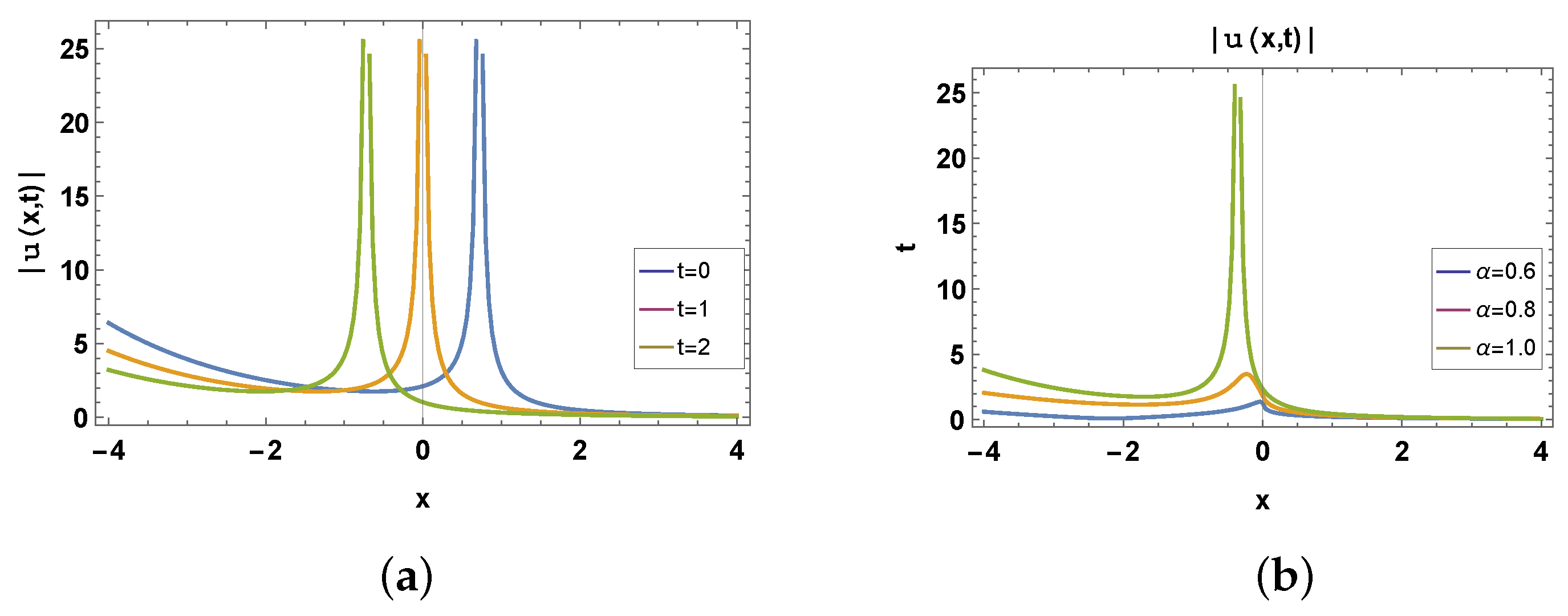
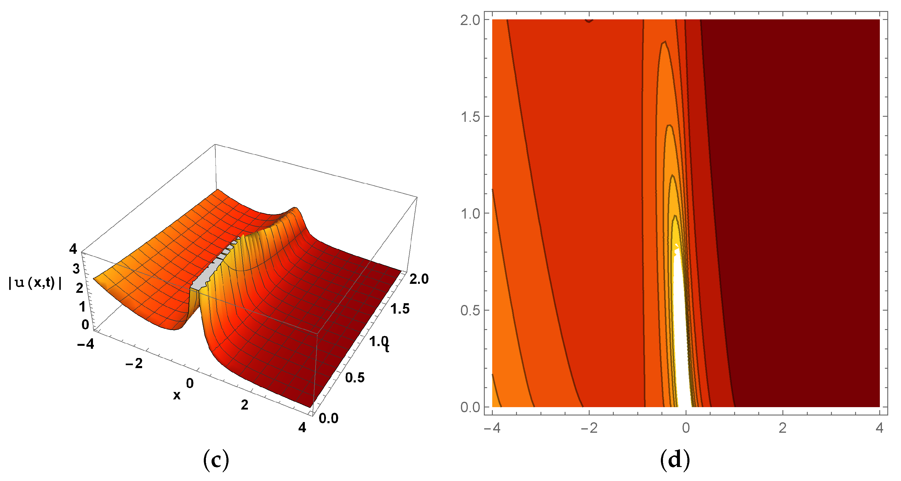
Here, we illustrate some of our obtained solutions using different kinds of graphs. The effect of the fractional order is also shown by means of the graphs (Figure 1, Figure 2 and Figure 3).

Figure 1. Represents a wave function of $\left|u\right(x,t\left)\right|$ shown in Equation (110) for $c=0.2;\Omega =0.1;\lambda =1;d=5;\tau =0.5;{\beta }_0=0.1;{\beta }_1=0.5;ϵ=1;{\rm Y}=1;$ (a) $-5<x<5$ in 2-D for $\alpha =1$, blue curve drawn for $t=0$, orange curve drawn for $t=1$, green curve drawn for $t=2$, (b) $-5<x<5$ in 2-D for $0<t<2$, blue curve drawn for $\alpha =0.6$, orange curve drawn for $\alpha =0.8$, green curve drawn for $\alpha =1$, (c) in 3-D for $\alpha =0.8$ and $0<t<2$, and (d) in the contour for $\alpha =0.8$ and $0<t<2$.

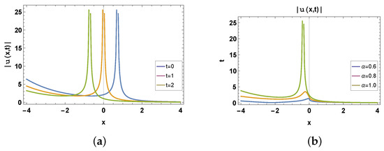
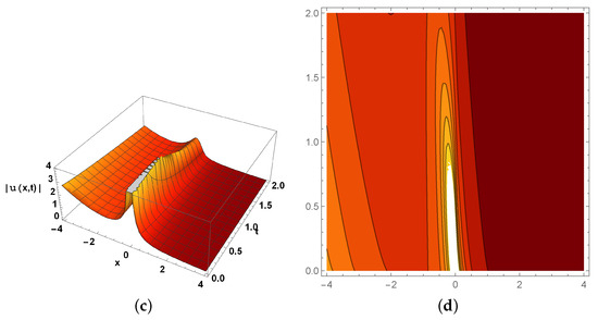
Figure 2. Represents a wave function of $\left|u\right(x,t\left)\right|$ shown in Equation (117) for $c=0.03;\Omega =0.6;\lambda =0.1;\tau =0.5;ϵ=1;{\rm Y}=1;$(a) $-4<x<4$ in 2-D for $\alpha =1$, blue curve drawn for $t=0$, orange curve drawn for $t=1$, green curve drawn for $t=2$, (b) $-4<x<4$ in 2-D for $0<t<2$, blue curve drawn for $\alpha =0.6$, orange curve drawn for $\alpha =0.8$, green curve drawn for $\alpha =1$, (c) in 3-D for $\alpha =0.8$ and $0<t<2$, and (d) in the contour for $\alpha =0.8$ and $0<t<2$.

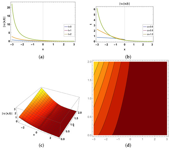
Figure 3. Represents a wave function of $\left|u\right(x,t\left)\right|$ shown in Equation (142) for $c=0.03;\Omega =0.5;\lambda =0.5;\tau =0.5;\omega =0.6;\sigma =0.5;\rho =0.5;d_0=1;ϵ=1;{\rm Y}=1;$(a) $-3<x<3$ in 2-D for $\alpha =1$, blue curve drawn for $t=0$, orange curve drawn for $t=1$, green curve drawn for $t=2$, (b) $-4<x<4$ in 2-D for $0<t<2$, blue curve drawn for $\alpha =0.6$, orange curve drawn for $\alpha =0.8$, green curve drawn for $\alpha =1$, (c) in 3-D for $\alpha =0.8$ and $0<t<2$, and (d) in the contour for $\alpha =0.8$ and $0<t<2$.

10. Conclusions

In this article, we obtain new analytical wave solutions to the Kuralay-II equations along the truncated M-fractional derivative by utilizing the ${exp}_a$ function, the extended sinh-Gordon equation expansion, and the generalized Kudryashov schemes. These results are also verified and explained with 2-D, 3-D and contour plots using the Mathematica tool in Figure 1, Figure 2 and Figure 3. The constraints on the parameters are considered to secure the existence of the obtained solitons. This work could be expanded in the future to include optical couplers, metamaterials, and fractional order integrable Kuralay Equations. Fractional derivatives, specifically, the truncated M-fractional derivative, are used for the first time in this model. The fractional-order derivative provides more accurate and appropriate solutions than the classical-/integer- order derivatives. The solutions obtained through the truncated M-fractional derivative are the closest to the approximate results/experimental results. The analytical wave solutions are highly desirable as they offer insights into this model for use in various fields, like nonlinear optics, ferromagnetic materials and optical fibers. Finally, it is suggested that, for dealing with other non-linear PDEs, the ${exp}_a$ function, the extended sinh-Gordon equation expansion, and the generalized Kudryashov schemes are very helpful, reliable and straightforward to apply. The results obtained in this paper may be useful for facilitating progress in the further analysis of this model applied to nonlinear optics, ferromagnetic materials and optical fibers.

References

- Ghanbari, B.; Osman, M.S.; Baleanu, D. Generalized exponential rational function method for extended Zakharov–Kuzetsov equation with conformable derivative. Mod. Phys. Lett. A 2019, 34, 1950155. [Google Scholar] [CrossRef]
- Akbulut, A.; Taşcan, F.; Özel, E. Trivial conservation laws and solitary wave solution of the fifth order Lax equation. Partial Differ. Equ. Appl. Math. 2021, 4, 100101. [Google Scholar] [CrossRef]
- Khatri, H.; Gautam, M.S.; Malik, A. Localized and complex soliton solutions to the integrable (4 + 1)-dimensional Fokas equation. SN Appl. Sci. 2019, 1, 1070. [Google Scholar] [CrossRef]
- Alam, M.N.; İlhan, O.A.; Uddin, M.S.; Rahim, M.A. Regarding on the Results for the Fractional Clannish Random Walker’s Parabolic Equation and the Nonlinear Fractional Cahn-Allen Equation. Adv. Math. Phys. 2022, 2022, 5635514. [Google Scholar] [CrossRef]
- Alam, M.N.; Islam, S.; İlhan, O.A.; Bulut, H. Some new results of nonlinear model arising in incompressible visco-elastic Kelvin–Voigt fluid. Math. Methods Appl. Sci. 2022, 45, 10347–10362. [Google Scholar] [CrossRef]
- Younas, U.; Seadawy, A.R.; Younis, M.; Rizvi, S.T.R. Optical solitons and closed form solutions to the (3 + 1)-dimensional resonant Schrödinger dynamical wave equation. Int. J. Mod. Phys. B 2020, 34, 2050291. [Google Scholar] [CrossRef]
- Rizvi, S.T.R.; Seadawy, A.R.; Ahmed, S.; Younis, M.; Ali, K. Study of multiple lump and rogue waves to the generalized unstable space time fractional nonlinear Schrödinger equation. Chaos Solitons Fractals 2021, 151, 111251. [Google Scholar] [CrossRef]
- Seadawy, A.R.; Iqbal, M.; Lu, D. Applications of propagation of long-wave with dissipation and dispersion in nonlinear media via solitary wave solutions of generalized Kadomtsev–Petviashvili modified equal width dynamical equation. Comput. Math. Appl. 2019, 78, 3620–3632. [Google Scholar] [CrossRef]
- Arshad, M.; Seadawy, A.; Lu, D.; Wang, J. Travelling wave solutions of generalized coupled Zakharov–Kuznetsov and dispersive long wave equations. Results Phys. 2016, 6, 1136–1145. [Google Scholar] [CrossRef]
- Rani, M.; Ahmed, N.; Dragomir, S.S.; Mohyud-Din, S.T.; Khan, I.; Nisar, K.S. Some newly explored exact solitary wave solutions to nonlinear inhomogeneous Murnaghan’s rod equation of fractional order. J. Taibah Univ. Sci. 2021, 15, 97–110. [Google Scholar] [CrossRef]
- Kumar, S.; Nisar, K.S.; Niwas, M. On the dynamics of exact solutions to a (3 + 1)-dimensional YTSF equation emerging in shallow sea waves: Lie symmetry analysis and generalized Kudryashov method. Results Phys. 2023, 48, 106432. [Google Scholar] [CrossRef]
- Irshad, A.; Ahmed, N.; Nazir, A.; Khan, U.; Mohyud-Din, S.T. Novel exact double periodic Soliton solutions to strain wave equation in micro structured solids. Phys. Stat. Mech. Appl. 2020, 550, 124077. [Google Scholar] [CrossRef]
- Ellahi, R.; Mohyud-Din, S.T.; Khan, U. Exact traveling wave solutions of fractional order Boussinesq-like equations by applying Exp-function method. Results Phys. 2018, 8, 114–120. [Google Scholar]
- Bibi, S.; Mohyud-Din, S.T.; Khan, U.; Ahmed, N. Khater method for nonlinear Sharma Tasso-Olever (STO) equation of fractional order. Results Phys. 2017, 7, 4440–4450. [Google Scholar] [CrossRef]
- Irshad, A.; Mohyud-Din, S.T.; Ahmed, N.; Khan, U. A new modification in simple equation method and its applications on nonlinear equations of physical nature. Results Phys. 2017, 7, 4232–4240. [Google Scholar] [CrossRef]
- Dahiya, S.; Kumar, H.; Kumar, A.; Gautam, M.S. Optical solitons in twin-core couplers with the nearest neighbor coupling. Partial. Differ. Equ. Appl. Math. 2021, 4, 100136. [Google Scholar]
- El-Ganaini, S.; Ma, W.-X.; Kumar, H. Modulational instability, optical solitons and travelling wave solutions to two nonlinear models in birefringent fibres with and without four-wave mixing terms. Pramana 2023, 97, 119. [Google Scholar] [CrossRef]
- El-Ganaini, S.; Kumar, H. A variety of new soliton structures and various dynamical behaviors of a discrete electrical lattice with nonlinear dispersion via variety of analytical architectures. Math. Methods Appl. Sci. 2023, 46, 2746–2772. [Google Scholar] [CrossRef]
- Alam, M.N. An analytical method for finding exact solutions of a nonlinear partial differential equation arising in electrical engineering. Open J. Math. Sci. 2023, 7, 10–18. [Google Scholar] [CrossRef]
- Ali, A.T.; Hassan, E.R. General expa function method for nonlinear evolution equations. Appl. Math. Comput. 2010, 217, 451–459. [Google Scholar] [CrossRef]
- Yan, C. A simple transformation for nonlinear waves. Phys. Lett. A 1996, 22, 77–84. [Google Scholar] [CrossRef]
- Zafar, A.; Bekir, A.; Raheel, M.; Rezazadeh, H. Investigation for optical soliton solutions of two nonlinear Schrödinger equations via two concrete finite series methods. Int. J. Appl. Comput. Math. 2020, 6, 65. [Google Scholar] [CrossRef]
- Chen, Z.; Manafian, J.; Raheel, M.; Zafar, A.; Alsaikhan, F.; Abotaleb, M. Extracting the exact solitons of time-fractional three coupled nonlinear Maccari’s system with complex form via four different methods. Results Phys. 2022, 36, 105400. [Google Scholar] [CrossRef]
- Aljoudi, S. Exact solutions of the fractional Sharma-Tasso-Olver equation and the fractional Bogoyavlenskii’s breaking soliton equations. Appl. Math. Comput. 2021, 405, 126237. [Google Scholar] [CrossRef]
- Kudryashov, N.A. One method for finding exact solutions of nonlinear differential equations, Commun. Nonlinear Sci. Numer. Simul. 2012, 17, 2248–2253. [Google Scholar] [CrossRef]
- Gaber, A.A.; Aljohani, A.F.; Ebaid, A.; Machado, J.T. The generalized Kudryashov method for nonlinear space–time fractional partial differential equations of burgers type. Nonlinear Dyn. 2019, 95, 361–368. [Google Scholar] [CrossRef]
- Barman, H.K.; Roy, R.; Mahmud, F.; Akbar, M.A.; Osman, M.S. Harmonizing wave solutions to the Fokas-Lenells model through the generalized Kudryashov method. Optik 2021, 229, 166294. [Google Scholar] [CrossRef]
- Pandir, Y.; Sahragül, E.R.E.N. Exact solutions of the two dimensional KdV-Burger equation by generalized Kudryashov method. J. Inst. Sci. Technol. 2021, 11, 617–624. [Google Scholar] [CrossRef]
- Sagidullayeva, Z.; Nugmanova, G.; Myrzakulov, R.; Serikbayev, N. Integrable Kuralay equations: Geometry, solutions and generalizations. Symmetry 2022, 14, 1374. [Google Scholar] [CrossRef]
- Faridi, W.A.; Bakar, M.A.; Myrzakulova, Z.; Myrzakulov, R.; Akgül, A.; El Din, S.M. The formation of solitary wave solutions and their propagation for Kuralay equation. Results Phys. 2023, 52, 106774. [Google Scholar] [CrossRef]
- Mathanaranjan, T. Optical soliton, linear stability analysis and conservation laws via multipliers to the integrable Kuralay equation. Optik 2023, 290, 171266. [Google Scholar] [CrossRef]
- Sulaiman, T.A.; Yel, G.; Bulut, H. M-fractional solitons and periodic wave solutions to the Hirota–Maccari system. Mod. Phys. Lett. B 2019, 33, 1950052. [Google Scholar] [CrossRef]
- Sousa, J.V.D.A.C.; De Oliveira, E.C. A new truncated M-fractional derivative type unifying some fractional derivative types with classical properties. Int. J. Anal. Appl. 2018, 16, 83–96. [Google Scholar]
- Zayed, E.M.E.; Al-Nowehy, A.G. Generalized kudryashov method and general expa function method for solving a high order nonlinear schrödinger equation. J. Space Explor. 2017, 6, 120. [Google Scholar]
- Hosseini, K.; Ayati, Z.; Ansari, R. New exact solutions of the Tzitzéica-type equations in non-linear optics using the expa function method. J. Mod. Opt. 2018, 65, 847–851. [Google Scholar] [CrossRef]
- Yang, X.L.; Tang, J.S. Travelling wave solutions for Konopelchenko-Dubrovsky equation using an extended sinh-Gordon equation expansion method. Commun. Theor. Phys. 2008, 50, 10471051. [Google Scholar]
- Gómez, C.A.; Salas, A.H. Special symmetries to standard Riccati equations and applications. Appl. Math. Comput. 2010, 216, 3089–3096. [Google Scholar] [CrossRef]
Disclaimer/Publisher’s Note: The statements, opinions and data contained in all publications are solely those of the individual author(s) and contributor(s) and not of MDPI and/or the editor(s). MDPI and/or the editor(s) disclaim responsibility for any injury to people or property resulting from any ideas, methods, instructions or products referred to in the content. |
© 2023 by the authors. Licensee MDPI, Basel, Switzerland. This article is an open access article distributed under the terms and conditions of the Creative Commons Attribution (CC BY) license (https://creativecommons.org/licenses/by/4.0/).