1. Introduction
Everyday life requires finding optimal solutions in a faster way to reduce costs and computational times, and to increase productivity or revenues. Finding the best or less costly route, setting up an optimal schedule, reducing production times, and controlling engineering systems are some examples of optimization problems. Therefore, optimization techniques are relevant in broad areas of life, which makes the continuous research and improvement in existing algorithms necessary [
1,
2,
3,
4].
Global optimization is concerned with finding the global solution for which the objective function obtains its smallest value. Formally, global optimization seeks a global solution of a constrained optimization model.
When only one function is optimized, the problem is referred to as a single objective optimization problem, while if two or more fitness functions are optimized, it is called a multiobjective problem.
The fitness function is regarded as a mapping , where is a multidimensional decision variable, and is part of the objective space . Thus, we have a mapping . Given a function , the solution to the optimization problem is a vector , such that the fitness function is close to its optimum value, i.e., it satisfies , where is the vector that gives the minimum or maximum value of the objective function, that is, the vector that minimizes or maximizes the objective function.
Among others, metaheuristic methods are efficient techniques to solve optimization problems [
5]. These methods use an iterative process to improve an initial solution up to a selected termination criterion, within a reasonable time and with low computational costs. There are several classifications for metaheuristics; Beheshti et al. [
6] classify them as nature [
1,
7,
8,
9,
10,
11,
12,
13,
14,
15,
16,
17] and non-nature inspired [
2,
18,
19,
20], population-based, single point search, dynamic and static objective function, single and various neighborhood structures, and memory usage and memory-less methods, among others.
Population-based metaheuristic algorithms have been broadly studied for global searches, as they can handle high-dimensional optimization problems. They present exploration and exploitation capabilities where exploration is related to the generation of new individuals in unexplored regions of the search space, while exploitation focuses the search in the neighborhood of known solutions [
21]. Too much of the former can lead to an inefficient search, and too much of the latter can lead to a propensity to focus the search too quickly, losing many possible solutions [
22].
A good balance between exploration and exploitation is required to avoid the trapping of the particles into local optima (premature convergence), and to find a good optimal solution in a few iterations [
23]. Recent works try to incorporate local search with exploration to achieve the better performance of the algorithms. The most popular heuristic algorithms are the particle swarm optimization algorithm (PSO) [
18,
24,
25] and the Differential Evolution Algorithm [
26,
27], which have been modified numerous times to improve their local and global search capabilities [
28,
29,
30]. In a study by Sun et al. [
31], the Whale Optimization Algorithm (WOA) is modified to perform a more detailed local search. The Butterfly Optimization Algorithm (BOA) is also improved by Li et al. [
1] to achieve a balance between exploration and exploitation. The Polar Bear Optimization Algorithm (PBO) [
9] was proposed, taking into account an efficient birth and death mechanism to improve global and local search.
In recent years, new algorithms have been proposed with new local and global search models, some examples of these are: Artificial ecosystem-based optimization (AEO) [
32], Jellyfish-inspired metaheuristic (JF) [
33], Chaos Game Oprimizer (CGO) [
34], Zebra Optimization Algorithm (ZOA), [
35], Chameleon Swarm Algorithm (CSA) [
36], Serval Optimization Algorithm (SOA) [
37], optimization problems based on walruses behavior (OWB) [
38], LSHADE-SPACMA Algorithm [
39], Coronavirus Optimization Algorithm (COA) [
40], Gaining-Sharing Knowledge Based Algorithm With Adaptive Parameters (APKBS) [
41], and Improving Multi-Objective Differential Evolution Algorithm (IMODE) [
42], etc.
Some of the most efficient metaheuristics are the Evolutionary Algorithms (EAs), which are flexible enough to solve different types of problems due to their exploration and exploitation capabilities. They are distinguished from Genetic Algorithms (GA) in the way they combine information through evolutionary operators that evolve the population, obtaining a set of new solutions [
43]. These methods can solve problems of high computational complexity or high dimensional problems.
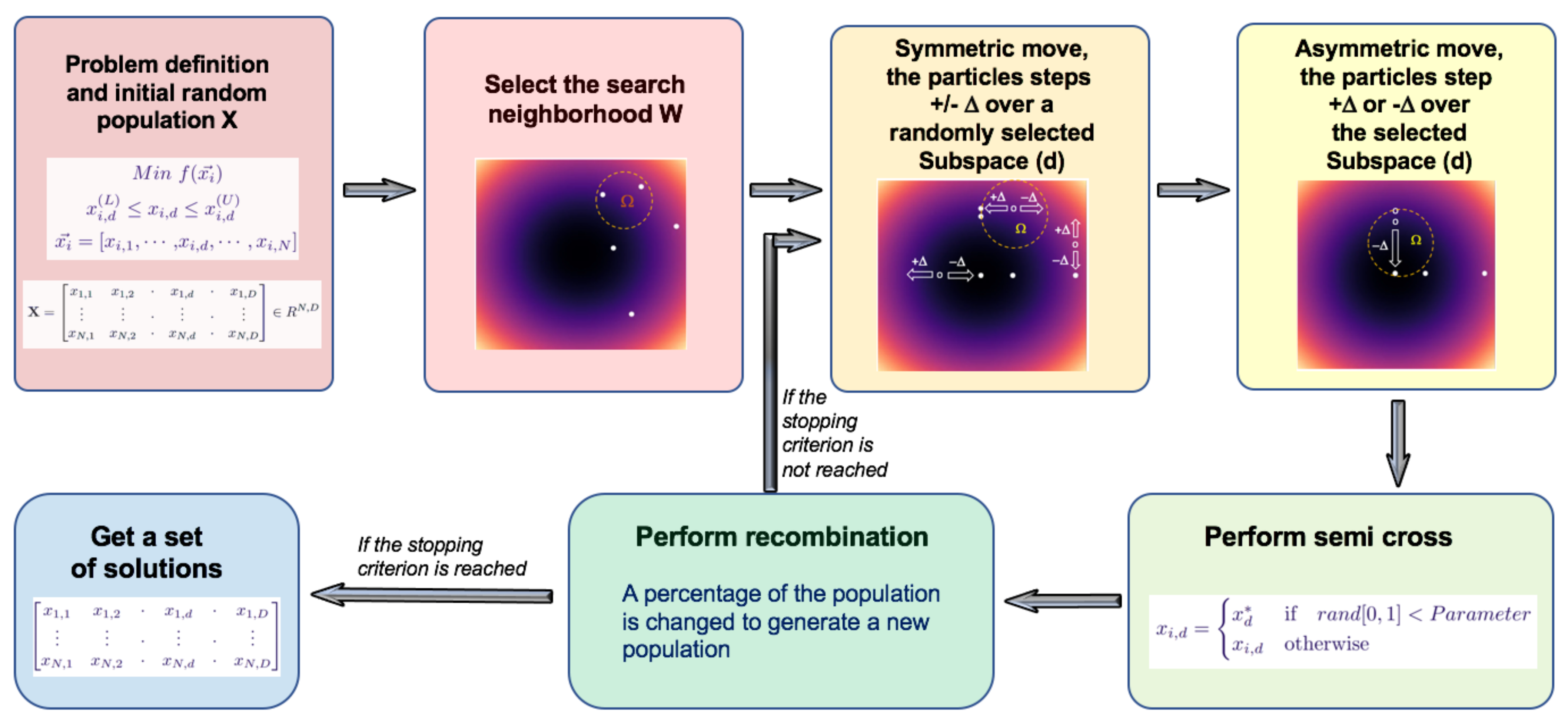
This work proposes a novel optimization method of the evolutionary type: the One-Dimensional Subspaces Optimization Algorithm (1D-SOA). This algorithm performs an exhaustive local search or exploitation, by updating the position of each individual of a randomly generated population, over a selected direction. This search generates a large number of optimal local sets. The search neighborhood is changed randomly, increasing, in this way, the local search space. Nevertheless, this is not the only characteristic of the algorithm. During the whole process, it also performs exploration, by generating diversity via the recombination of the initial population, which favors a convergence towards the global optimum. The algorithm is tested for single-objective optimization problems. More details of the algorithm are presented in
Section 3.
This work is structured as follows, in
Section 2, the theory related to single objective optimization problems is presented. Later, in
Section 3, 1D-SOA is introduced, together with details about its implementation and some EAs used for comparison. After that, the results and discussion are presented in
Section 4. Finally, the conclusions and references are given in
Section 5.
4. Results and Discussion
This section contains the results of the experiments performed to study the behavior of the 1D-SOA algorithm introduced in this work. The performance of 1D-SOA was compared against the heuristic algorithms from the python library SwarmPackagePy [
49]; in particular, the studied algorithms from this library are Artificial Bee Algorithm (ABA) [
50], Bat Algorithm (BA) [
51], Bacterial Foraging Optimization (BFO) [
52], Cat Swarm Optimization (CA) [
17], Chicken Swarm Optimization (CHSO) [
10], Cuckoo Search Optimization (CU) [
13], Firefly algorithm (FA) [
15], Fireworks Algorithm (FWA) [
20], Gravitational Search Algorithm (GSA) [
19], Grey Wolf Optimizer (GWO) [
19], Particle Swarm Optimization (PSO) [
18], and Social Spider Algorithm (SSA) [
14]. Additionally, we include in the comparison some state-of-the-art algorithms: Mean particle Swarm Optimisation (MPSO) [
53], Artificial ecosystem-based optimization (AEO) [
32], Jellyfish inspired metaheuristic (JF) [
33], Chaos Game Optimizer (CGO) [
34], and Zebra Optimization Algorithm (ZOA) [
35].
All algorithms require a basic number of input parameters: the number of individuals (N), dimension (D), number of maximum iterations (
), and lower (
) and upper (
) limits in the search space. Additionally, some algorithms need a specific set of extra control parameters.
Table 2 shows the specific parameters, together with the most common values used in the literature and this work. A brief discussion of the selection of parameters used for the MPSO, FWA, and CHSO is presented in
Appendix A. For the 1D-SOA Algorithm, besides the parameters presented in the above-mentioned table, it is required to define the following fixed variables,
,
,
,
, and
that we recommend not to change, as they work for all the studied problems. The 30 studied benchmark functions are presented in the
Appendix C,
Table A8,
Table A9 and
Table A10. This table contains the search space, the optimal solution vector
, and the function evaluated at this vector
, i.e., the optimum. Additionally, for the 1D-SOA method, it is required to select two parameters,
and
; the values of these parameters are presented in the same tables.
The comparison was made for different dimensions, in particular .
For the experiments, a statistical analysis of the performance of the algorithms was performed and the algorithms were compared from 100 runs for each function. From the 100 runs, the best solution and the mean of the 100 runs were obtained for the statistic at an approximated value of ; for the functions that do not reach this value, the 100 iterations were taken.
The initial population varied for each dimension; for dimensions less or equal to 10 the initial population was 10, while for larger dimensions the initial population corresponds to the dimension. Next, we present the results for dimensions 2 and 30.
In
Figure 2, all the algorithms are presented for 30 D for the ackley, ackley_2, rastrigin, and schwefel 2.20 functions. It can be noticed that the algorithms with slightly better performance are: 1D-SOA, FWA, ZOA, AEO, MPSO, and CHSO. For the rest of the algorithms, most of the time they do not converge in the required number of iterations. Therefore, to have more clarity in the plots and tables, only the algorithms mentioned above are presented. In
Figure 3 and
Figure 4, the convergence for different steps for six search directions, and for various search directions and five steps, are presented. It is worth noticing from the plots that the convergence slightly improves with more search steps and more search directions. However, the computational work increases, therefore the parameters selected were five steps and 20% of the dimensions as search dimensions, as these parameters have a good balance between work and performance (see
Table 1).
4.1. Results for 2D Experiments
The complete results of this section are presented in the
Appendix B,
Table A1,
Table A2 and
Table A3, that show the value that reaches the best solution out of the 100 runs, the averaged value reached, and the standard deviation for all the algorithms. The algorithm with the best performance has the darker corresponding value. If two algorithms have the same value, the one with faster convergence in the plots is selected. Additionally, two statistical tests were performed and included in these tables, the
t-test [
23], and the alternative to the Mann–Witney U Test, suggested by Mark Wineberg and Steffen Christensen, that is a non-parametric test based on the ranking of the results [
54]. According to the non-parametric tests performed, most of the freedom degrees are close to 100, and the t statistic ranges from 3.3 to 49, which, from the Tables given in [
54], indicates that the probability that the null hypotheses is wrong is over 99.8%; this implies that our results can be trusted. A summary of the results obtained for dimension 2 is presented in
Table 3. In this table, we can observe that the best performance for the best solution was obtained for the 1D-SOA, while for the mean of the solutions, the best performance was achieved by the FWA. The convergence of the algorithms 1D-SOA, FWA, ZOA, AEO, MPSO, and CHSO for some functions is shown in
Figure 5.
From the figures, it was observed that there exist two different behaviors of the algorithms depending on the function. For the first kind, all the algorithms converge at a similar rate, this behavior is observed for most of the functions, in particular, the functions: , , , , , , , , , , , , , , , , , , , , , and . For the second kind, the convergence is very slow for all the algorithms, except for one or two algorithms; this happens for functions , , , , , , , , and .
4.2. Results for 30D
The complete results of this section are presented in the
Appendix B,
Table A4,
Table A5 and
Table A6, that show the value that reaches the best solution out of the 100 runs, the averaged value reached, and the standard deviation for all the algorithms. As in the previous case (2D), the two statistical tests were performed and included in the tables. According to the non-parametric tests performed, most of the freedom degrees are close to or larger than 100, and the t statistic ranges from 3.7 to 52, which, from Tables [
54], indicates that the probability that the null hypothesis is wrong is over 99.8%; this implies that our results can be trusted. A summary of the results obtained for dimension 30 is presented in
Table 4. This table shows that the best performance for the best and mean solution was obtained for the 1D-SOA, followed by the FWA. The convergence of the algorithms 1D-SOA, FWA, ZOA, AEO, MPSO, and CHSO for some functions is shown in
Figure 6.
For 30D, the CHSO algorithm shows a general performance that is worse than the 2D case. As in the previous case, different behaviors of the algorithms depending on the function are observed. For most of the functions, the convergence is similar for all the algorithms, in particular, for the functions: , , , , , , , , , , and . There is also a case where the 1D-SOA, FWA, ZOA, AEO, and MPSO present similar performances, but the CHSO fails to converge, the functions with this behavior are: , , , , , , , , , , and . Finally, there is a case where only one or two functions converge or converge faster than the rest, this happens for functions: , , , , , , and . For functions and , 1D-SOA does not converge. However, for functions , , , and only 1D-SOA converges.
4.3. Experiments with Functions with the Optimal Solution Not in Zero
The minimal value of the functions studied in the previous sections have a minimum
located in
However, some of them have the optimum in a different position. In this section, the functions with a non-zero optimum are studied; they are presented in
Table A11, together with their optimal value. The functions
and
can be generalized to D dimensions and they are studied in the previous section; only the minimum value was shifted to zero, therefore we only show their convergence plots if they are not shifted towards zero in
Figure 7. The rest of the functions are only defined in 2D. The results are presented in
Table A7. For some of the functions studied in this section, the CHSO algorithm showed problems computing the solution, therefore, the studied algorithms are 1D-SOA, FWA, ZOA, AEO, and MPSO. The convergence plots are presented in
Figure 8.
Regarding the best value, for these functions, most of the results are similar for all the algorithms, except for and , where FWA for and 1D-SOA for converge slightly faster than the rest to the optimum. For the Mean value, FWA reaches values closer to the optimum.
5. Conclusions
This work introduces the one-dimensional search optimization algorithm (1D-SOA) for solving optimization problems. This algorithm optimizes an initial population over a randomly selected dimension. It selects the search direction by moving symmetrically in the one-dimensional subspace (1D-S) created by the selected dimension. After the direction of the search is selected, the individuals move asymmetrically to find the local optima in the 1D-S. The algorithm includes exploitation by diminishing the size of the step to perform a local search. It also performs exploration by recombining the particles. To study the performance and efficiency of the proposed algorithm, it was compared against another 11 algorithms for 30 benchmark functions for various dimensions.
The comparison was made for two cases: (1) the best values reached by the algorithms, and (2) the mean performance out of 100 runs. For the best value, the best performance was observed for the 1D-SOA, for which 43.3% of the functions were in 2D, 70% in 30D; followed by the FWA with 26.6% in 2D, 16.6% in 30D; the CHSO with 20% in 2D; and the AEO with 6.6% in 30D. For the mean convergence, FWA showed a better performance with 53.3%, followed by the 1D-SOA with 33.3% of the functions in 2D. In 30D, the best performance was observed by the 1D-SOA algorithm with 63.3%, followed by the FWA with 33.3%. A t-test and a non-parametric test were performed to check the validity of the results.
The functions with non-zero optimum were studied for 2D, and the results were similar for the best solution except for the and functions, where the best performance was obtained with the FWA and the 1D-SOA algorithms. The FWA showed the best performance for the mean solutions.
From the results, it can be concluded that the best performance was achieved with the proposed algorithm (1D-SOA) in 30D, followed by the fireworks algorithm (FWA). For most of the functions, the convergence was similar for 2D. However, for larger dimensions, the chicken swarm optimization (CHSO) algorithm worsens its performance, while 1D-SOA showed a better performance. Furthermore, for some functions, 1D-SOA was the only algorithm that converged in large dimensions.
A fixed set of parameters was chosen for 1D-SOA to compare it against the other algorithms. However, these parameters can be adapted for diverse optimization problems. It is suggested to carry out an analysis of the parameters to find the most adequate ones for a given problem.


