Article

Estimation of Multiple Breaks in Panel Data Models Based on a Modified Screening and Ranking Algorithm

1
Faculty of Science, Xi’an University of Technology, Xi’an 710048, China
2
School of Mathematics and Statistics, Qinghai Normal University, Xining 810008, China
3
Academy of Plateau Science and Sustainability, Xining 810008, China
*
Author to whom correspondence should be addressed.
Symmetry 2023, 15(10), 1890; https://doi.org/10.3390/sym15101890
Submission received: 1 September 2023 / Revised: 24 September 2023 / Accepted: 3 October 2023 / Published: 9 October 2023
(This article belongs to the Special Issue Symmetry in Probability Theory and Statistics)

Abstract

:
Structural breaks are often encountered in empirical studies with large panels. This paper considers the estimation of multiple breaks in the mean of panel data model based on a modified screening and ranking algorithm. This algorithm satisfies symmetry and is suitable for both cases where the jump size of break points is positive and negative. The break points are first initially screened based on the adaptive Fisher’s statistic, followed by further screening of the break points using the threshold criterion, and finally the final break points are screened using the information criterion. Furthermore, the consistency of the break point estimators is proved. The Monte Carlo simulation results show that the proposed method performs well even if the error terms are serially correlated or cross-sectionally correlated. Finally, two empirical examples illustrate the use of this method.

1. Introduction

Structural breaks are a common feature in many fields of economics. For example, in macroeconomics, the process of GDP, inflation and the interest rate are often vulnerable to political, technological and supply shocks, resulting in structural breaks. Ignoring structural breaks could lead to completely different or, more seriously, misleading conclusions in policy evaluations. Estimating the point at which a structural break occurs in time series models has been extensively researched. We refer the reader to Csörgö and Horváth [1], Bai and Perron [2], Perron [3], Gombay [4], Chen et al. [5], Chen [6], Zou et al. [7,8], Wang et al. [9], Tveten et al. [10] for comprehensive surveys.
In recent years, there has been a growing amount of literature on estimating structural breaks in panel data models. Bai [11] estimated the break points in the mean and variance of the panel data model using the least squares method and the quasi-maximum likelihood method. Kim [12] investigated the estimation of the common deterministic time trend break in large panels by minimizing the sum of squared residuals for all possible break points. Kim [13], continued from [12], considered the joint estimation of the common break point and the common factors for large panels. Peštová and Pešta [14] considered a ratio type test statistic to detect a possible common break in means of the panels, and introduced a common break point estimation. Baltagi et al. [15] studied the estimation of a common structural break in large heterogeneous panels with a general multifactor error structure using the least squares method. Xu et al. [16] proposed a class of weighed difference of average statistics to estimate the variance breaks in dependent panel data. When the correlation between cross-sectional individuals exists in the form of a common factor, Horvath et al. [17] proposed a CUSUM type statistic to estimate the breaks in the mean of panel data. For estimating structural breaks in linear panel data models with a grouped pattern of heterogeneity, Lumsdaine et al. [18] simultaneously estimated the break point, the group membership structure, and the coefficients based on the least squares method.
A common feature of the above work is the assumption of a single break in the estimation methodology. While assuming a single break simplifies estimation and inference, inference based on a single break can be misleading if the model has an unknown number of breaks. Therefore, many researchers have also studied multiple break point estimation in panel data. Supposing that the number of breaks in panel data models is given, Bai [11] and Feng [19] estimated multiple break points one by one based on the least squares method. Li et al. [20] proposed a penalized principal component estimation procedure that uses adaptive group fused Lasso to detect multiple structural breaks in panel data models with unobservable interaction fixed effects. Qian and Su [21] considered the estimation and inference of multiple breaks in the panel data model through the adaptive group fused Lasso. Okui and Wang [22] developed a method for estimating heterogeneous structural breaks in panel data models by grouped fixed effects and adaptive group fused Lasso. Kaddoura and Westerlund [23] investigated the estimation of multiple structural breaks for panel data models with random interactive effects using the Lasso method.
The above literature studied the estimation of multiple structural breaks in panel data regression models, and the research on the estimation of multiple breaks in the mean of panel data models is as follows. Bai [11] studied the estimation of multiple breaks in panel data models by the least squares method, but the number of breaks needs to be known in advance. Cho [24] provided a double CUSUM binary segmentation algorithm for detecting multiple breakpoints in panel data models. Based on the idea of the screening and ranking algorithm, Song et al. [25] studied the estimation of multiple break points in multiple samples based on the adaptive Fisher method. The screening and ranking algorithm (SaRa) originated from the estimation of multiple break points in time series models. To reduce the computational complexity, Niu and Zhang [26] proposed a fast and local algorithm based on a local diagnostic statistic to estimate multiple break points in a time series model. It has a computational complexity of as low as O ( T ) . Hao et al. [27] discussed the theoretical properties of SaRa and showed its advantages over other algorithms. Xiao et al. [28] adopted a multiple-bandwidth strategy and a mixture model-based clustering to improve the performance of SaRa.
When the error terms of a panel data model follow a normal distribution, the double CUSUM binary segmentation algorithm [24] and multiple sample SaRa [25] are effective in estimating multiple break points in the panel data model, but when there is serial correlation or cross-sectional correlation in the error terms, the estimation of multiple break points in the panel data model is poor. In this paper, we propose a modified SaRa that adds an information criterion to the multiple sample SaRa to further screen multiple break points in the mean of a panel data model. Simulation results indicate that the method in this paper is effective in estimating the break points even if the error terms are serially correlated or cross-sectionally correlated.
The rest of the paper is organized as follows. The model and assumptions are described in Section 2. Section 3 illustrates the SaRa method and proves the consistency of the break point estimators. In Section 4, we discuss the finite sample performance of SaRa through Monte Carlo simulations. Section 5 offers a real example to illustrate the effectiveness of SaRa. Section 6 concludes the paper.

2. The Model and Assumption

In this section, we focus on the problem of estimating multiple break points in the mean of panel data
Y i t = μ i t + e i t , i = 1 , 2 , , N , t = 1 , 2 , , T ,
where μ i t t = 1 T , i = 1 , , N are piecewise constant which share an unknown number of break points at unknown locations, e i t is the error process. We suppose there exist J break points in the mean of the panel data,
Y i t = μ i 1 + e i t , μ i 2 + e i t , μ i , J + 1 + e i t , t = 1 , 2 , , τ 1 , t = τ 1 + 1 , , τ 2 , t = τ J + 1 , , T ,
i = 1 , , N , where J = τ 1 , τ 2 , , τ J are unknown break points, 1 < τ 1 < τ 2 < < τ J < T . μ i j is the mean of Y i , τ j 1 , , Y i , τ j , j = 1 , 2 , , J + 1 , Y i , τ 0 = 1 , Y i , τ J + 1 = T . δ i j = μ i j μ i , j 1 , j = 2 , , J + 1 denotes the jump size of the break, which is assumed to be independent of error process e i t , and E μ i j μ i , j 1 2 is bounded for all i.
First, we assume that the error process e i t is stationary in the time dimension.
Assumption 1.
e i t = j = 0 a i j ε i , t j , ε i t i . i . d . N 0 , σ i ε 2 , j = 0 j a i j M for all i, M is a positive number. In addition, e i t are independent over i.
Assumption 1 means e i t are cross-sectionally independent. Furthermore, we let σ i 2 = E e i t 2 = σ i ε 2 j = 0 a i j 2 ; we also assume that there are no break points in the variance.
Second, we assume that the sequence length T and the set of break points J = τ 1 , τ 2 , , τ J are fixed. Regarding the jump size of the break points, the following assumption is made.
Assumption 2.
For each j, δ 1 j , , δ N j are independent and
δ i j = 0 with probability 1 π j , Δ j , with probability π j ,
where 1 j J , π j > 0 , Δ j are fixed and assumed unknown.
Assumption 2 implies that for each break point τ j , only a certain percentage of the panels undergo structural breaks, i.e., δ i j 0 is satisfied. Therefore, this assumption does not require that every series has a break point.

3. Method

3.1. SaRa for a Time Series Model

The SaRa was first proposed by Niu and Zhang [26] to detect break points in the mean of normal models.
y t = θ t + ε t , ε t i . i . d . N 0 , σ 2 , t = 1 , , T
and assume that
θ 1 = θ 2 = = θ τ 1 θ τ 1 + 1 = = θ τ 2 θ τ 2 + 1 = = θ τ J θ τ J + 1 = = θ T .
For a position t, we consider the locally defined statistic
D t , h = k = t + 1 t + h y k k = t h + 1 j y t h 1 , h t T h ,
where h is the bandwidth [27]. Next, we estimate the break points based on D t , h in two steps. The first step is to calculate D t , h at all positions and find all h local maximizers of D t , h . t is a h local maximizer if
D t , h D t , h , for all t t h , t + h .
The second step is to apply the threshold criterion
D t , h > λ
on all local maximizers to filter the corresponding break points. Thus,
J h , λ = τ ^ j : τ ^ j is a local maximizer of D t , h and D t , h > λ
is a set of break point estimators.
For any t, D t , h N 0 , 2 h σ 2 if there are no break points in window t h , t + h . Based on this, a standardized scan statistic can be defined as follows:
D ˜ t , h = h 2 σ ^ D t , h , h t T h ,
where σ ^ is an estimator of σ . In this paper, we assume that the number of break points J T ; the sample standard deviation of y t can be used as σ ^ .

3.2. SaRa for a Panel Data Model

Compared to the estimation of break points in time series models, estimating common break points by combining information from all individuals in the panel data is better. We let D ˜ i t , h be the scan statistic on the ith cross-section unit at time t, and
p i t , h = 2 1 Φ D ˜ i t , h ,
i = 1 , , N , t = 1 , , T . As discussed in Song et al. [25], we combine the p values of the scan statistics D ˜ i t , h instead of combining D ˜ i t , h directly, which improves the robustness of the break point estimators.
For given t and h, we let
X i t , h = log p i t , h
and
X i t , h = log p i t , h ,
where p i t , h are the order statistics of p i t , h in an ascending order. Under the null hypothesis of no change, X i t , h i . i . d . E x p 1 .
We define
V i t , h = j = 1 i X j t , h
and standardize V i t , h as
V ˜ i t , h = V i t , h k = 1 N w k , i k = 1 N w 2 k , i ,
where w k , i = min 1 , i i k k .
Similar to Song et al. [25], the adaptive Fisher statistic for the panel data model takes the following form:
W t , h = max 1 i N V ˜ i t , h , h t T h .
Then, the two steps of the SaRa for the panel data model are as follows. First, for a given bandwidth h, we calculate the summary scan statistic W t , h to find the local maximizers, t = h + 1 , , T h . t is a local maximizer if
W t , h W t , h for all t t h , t + h .
Second, we apply the threshold criterion
W t , h > λ
on the set consisting of local maximizers to screen out the final break points.
For the selection of the threshold λ , we can simply simulate the null distribution of W ( t , h ) through the assumption that Y i i . i . d . MVN 0 , I for 1 i N , where Y i = Y i 1 , Y i 2 , , Y i T T . Then, for significance level α , we can calculate the inverse function of the empirical distribution function of W ( t , h ) to obtain the threshold λ = F ^ 1 1 α , where F ^ · is the simulated empirical distribution function of W ( t , h ) , t is a local maximizer. Alternatively, we can also use the 1 α quantile of W ( t , h ) as a threshold.
The choice of bandwidth h can affect the estimation of multiple break points. The bandwidth is less important if the break points are far apart and the mean is significantly shifted at each break point. Otherwise, we need to be careful in choosing the bandwidth. As discussed by Niu and Zhang [26], we tend to use longer bandwidths for breakpoints where there are only small jumps in the mean, but when long bandwidths are used, there may be other break points in the interval t h , t + h . In practical applications, we can use multiple bandwidths to alleviate this difficulty.
The multiple-bandwidth SaRa is described as follows. First, we choose a few bandwidths, h 1 , , h K , and run SaRa for each of them. The break point estimators obtained for each bandwidth are then collected in to a candidate pool. To avoid duplication, if the distance between two different break points detected by different bandwidths is less than the smaller bandwidth, we keep the break points estimated by the longer bandwidth and delete the break points estimated by the shorter bandwidth. Second, similar to a single-bandwidth SaRa, a threshold criterion is applied to the candidate pool to screen out the final break points.
The simulation results show that for the panel data model, the multiple-bandwidth SaRa, while estimating various types of break points, results in spurious break points. Based on this, we propose a modified screening ranking algorithm, i.e., adding an information criterion (IC) to the multiple-bandwidth SaRa for further screening, which also incorporates the best subset selection method into the screening process.
I C J ˜ , J ˜ = σ ^ J ˜ 2 + c ln N T N T J ˜ + 1 ,
where σ ^ J ˜ 2 is the variance assuming J ˜ = τ ˜ 1 , τ ˜ 2 , , τ ˜ J ˜ are break points, J ˜ is the number of break points, c is a tuning parameter.
The detailed algorithm is described below.
  • Given a set of bandwidths h 1 , , h K , h 1 < h 2 < < h K . For each bandwidth h j , we compute the scan statistic W t , h j for t = h + 1 , , T h , j = 1 , , K .
  • We find the local maximizers for each bandwidth h j and form a set called L M j .
    L M j = t : W t , h j > W t , h j , t t h j , t + h j = τ ˜ 1 j , τ ˜ 2 j , , τ ˜ J ˜ j j ,
    j = 1 , , K , where J ˜ j is an estimator of the number of break points under the bandwidth h j .
  • Under the bandwidth h j , we utilize the threshold criterion to filter out the break points on the collection of local maximizers,
    W τ ˜ l j , h j > λ , 1 l J ˜ j ,
    and then we collect together the break points obtained under each bandwidth and denote them as M .
  • We remove duplicate break points in the set M , i.e., if the distance between two break points obtained from different bandwidths is less than the shorter bandwidth, we remove the break points obtained from the shorter bandwidth and keep the breakpoints obtained from the longer bandwidth, and denote the set of break points finally obtained as J = τ 1 , τ 2 , , τ J .
  • We obtain the final break point estimation J ^ by the best subset selection on the set J using the minimization information criterion
    J ^ , J ^ = arg min J J , 1 J J IC J , J = arg min J J , 1 J J σ ^ J 2 + c ln ( NT ) NT ( J + 1 )
    where J = τ 1 , τ 2 , , τ J J = τ 1 , τ 2 , , τ J .

3.3. Statistical Properties

In this section, we show that our proposed method can detect common break points in panel data models with high probability when the sample size N is large.
Theorem 1.
If Assumptions 1 and 2 hold, there exists suitable h and λ such that J ^ = τ ^ 1 , τ ^ 2 , , τ ^ J ^ satisfies
lim N P J ^ = J J J ^ ± h = 1 ,
where J ^ ± h j = 1 J ^ τ ^ j h , τ ^ j + h .
Similar to the proof of Theorem 1 in Niu and Zhang [26], to prove that the conclusion holds, it needs to be shown that for a given bandwidth h, there exists λ such that
P W t , h < λ 1 for any h flat point t , P W τ j , h < λ for any j 1 , 2 , , J
as N .
We suppose Z 0 N 0 , 1 and Z j has the same distribution as D ˜ i τ j , h , j = 1 , 2 , , J . We define f = log 2 1 Φ · ; then, we have
E f Z 0 3 and E f Z j 3 , j = 1 , 2 , , J exist , v 0 = E f z 0 < v j = E f z j for any j .
We let ξ = min 1 j J v j v 0 v j v 0 2 2 ; by the definition of statistic V ˜ i t , h , for a flat point t, V ˜ i t , h is the standardization of the sum of independent exponential random variables. We set λ = N ξ ;
P N ξ < V ˜ i t , h < N ξ 1 2 N π ξ 3 exp 1 2 N ξ 2 2 C 1 + N ξ 3 ;
then,
P W t , h < N ξ = P max 1 i N V ˜ i t , h < N ξ = P i = 1 N N ξ < V ˜ i t , h < N ξ .
Thus,
P W t , h < N ξ 1 2 N π ξ 3 exp 1 2 N ξ 2 2 N C 1 + N ξ 3 1 , as N .
For each j 1 , 2 , , J ,
P W τ j , h > N ξ P V ˜ N τ j , h > N ξ = 1 P N ξ < V ˜ N τ j , h < N ξ = 1 P ξ < 1 N i = 1 N f D ˜ i τ j , h v 0 < ξ 1 , as N .
Therefore, the theorem is proved.

4. Numerical Result

Assuming that there are break points in the mean of the panel data model, but the number of break points is unknown, we study the finite sample performance of the modified screening and ranking algorithm (SaRa-M) using Monte Carlo simulations and compare it to the double CUSUM statistic [24] and the multiple sample SaRa [25].
With respect to the SaRa, in order to filter as many break points as possible, we find the threshold λ as the minimum value of W ( t , h ) on the local maximizers by assuming that Y i i . i . d . MVN 0 , I , where Y i = Y i 1 , Y i 2 , , Y i T T , i = 1 , 2 , , N . Since the number of break points is unknown, we use multiple-bandwidth SaRa to estimate the break points, and the bandwidth h is set to 5 and 10. In addition to the bandwidth, the tuning parameter c also has a significant effect on the estimation results. Through a large number of simulations, it is found that c = 0.3 is appropriate when the estimator of the serial correlation coefficient is less than 0.3; otherwise, a c that equals the estimator of the serial correlation coefficient is appropriate. Therefore, the selection of c depends on the estimator of the serial correlation coefficient.
As discussed in Song et al. [25], for the multiple-sample SaRa, the threshold λ is chosen as the 95% quantile of the statistics on the local maximizers by assuming Y i i . i . d . MVN 0 , I for 1 i N ; h is also set to 5 and 10. Regarding the double CUSUM statistic, the break point detection is performed with T 1 / 2 ( φ = 1 2 ). All simulations are based on 1000 replications.
This section discusses two types of panel data models with break points: one with a single break point and the other with three break points.
Model I: Single break point
Y i t = μ i 1 + e i t , t = 1 , 2 , , τ 1 , μ i 2 + e i t , t = τ 1 + 1 , , T ,
i = 1 , , N , where τ 1 = T T 2 2 , x denotes the integer part of x.
Model II: Three break points
Y i t = μ i 1 + e i t , μ i 2 + e i t , μ i 3 + e i t , μ i 4 + e i t , t = 1 , 2 , , τ 1 , t = τ 1 + 1 , , τ 2 , t = τ 2 + 1 , , τ 3 , t = τ 3 + 1 , , T ,
i = 1 , , N , where τ 1 = T T 4 4 , τ 2 = T T 2 2 , τ 3 = 3 T 3 T 4 4 .
The sample size is set to N = 50 , 100 , T = 50 , 100 . For Model I, the proportion of the number of panels that are assumed to change is 30%. When t = 1 , , τ 1 , we set
μ i 1 = 0 , i = 1 , , N ;
t = τ 1 + 1 , , T , we set
μ i 2 = 1 , if the i th panel undergoes a structural break , 0 , otherwise .
For Model II, it is assumed that the proportion of the number of panels that change is 50%. When t = 1 , , T T 4 4 , we set
μ i 1 = 0 , i = 1 , , N ;
t = T T 4 4 + 1 , , T T 2 2 , we set
μ i 2 = 1 , if the i th panel undergoes a structural break , 0 , otherwise ;
t = T T 2 2 + 1 , , 3 T 3 T 4 4 , we set
μ i 3 = 0 , i = 1 , , N ;
t = 3 T 3 T 4 4 + 1 , , T , we set
μ i 4 = 1 , if the i th panel undergoes a structural break , 0 , otherwise .
The panels that change are drawn randomly from 1 , , N . e i t are generated from the following four models:
(i)
e i t i . i . d . N 0 , 1 , i = 1 , , N , t = 1 , , T ;
(ii)
e i t = v i t ε i t , where v i t 2 = 0.2 + 0.3 e i t 2 + 0.3 v i , t 1 2 , ε i t i . i . d . N 0 , 1 , i = 1 , , N , t = 1 , , T ;
(iii)
e i t = 0.5 e i , t 1 + ε i t , ε i t i . i . d . N 0 , 1 , i = 1 , , N , t = 1 , , T ;
(iv)
e i t = γ i f t + v i t , where γ i i . i . d . N 1 , 0.5 , f t i . i . d . N 0 , 0.2 , v i t i . i . d . N 0 , 1 , i = 1 , , N , t = 1 , , T .
(i) means that the error terms are independent and identically distributed; (ii) implies the error terms follow a GARCH(1, 1) model; (iii) and (iv) indicate that there is serial and cross-sectional correlation in the error terms, respectively.
The above panel data with common break points are very common in real life. For example, a credit crunch or a debt crisis may affect every company’s stock income, and fluctuations in the price of crude oil may affect every country’s exports. A change in tax policy could change every company’s investment strategy. Similarly, the emergence of a new technology, the introduction of a new drug, or the introduction of a new government program can have an impact on people’s lives and other economic entities. Estimating common break points using panel data makes the estimation more precise.
Table 1, Table 2, Table 3 and Table 4 show the simulation results of SaRa-M, DCUSUM and MSSaRa when e i t are generated as (i), (ii), (iii) and (iv), respectively. These include the percentage of correctly estimating the number of break points (single break point, J ^ = 1 ; three break points, J ^ = 3 , in %), the percentage of falsely estimating the number of break points (single break point, J ^ < 1 , J ^ > 1 ; three break points, J ^ < 3 , J ^ > 3 , in %), the mean Hausdorff distance (MHD) between the estimated break points and the true break points (Qian an Su [21]), and the location accuracy of break points (single break point, τ ^ 1 τ 1 < log T ; three break points, τ ^ 1 τ 1 < log T , τ ^ 2 τ 2 < log T , τ ^ 3 τ 3 < log T , in %, Cho [24]).
The simulation results show that for Model I and Model II, as the sample size increases, the percentage of the number of break points correctly estimated by SaRa-M, DCUSUM, and MSSaRa increases, the mean Hausdorff distance decreases, and the location accuracy increases. Compared to when the error terms are generated as (ii) or (iii) or (iv), the three methods have the best estimation results when the error terms are generated as (i), i.e., the percentage of correctly estimating the number of break points ( J ^ = 1 or J ^ = 3 ) is almost 100%, the mean Hausdorff distance (MHD) is the samllest, and the location accuracy is the highest.
In terms of the percentage of correct estimation of the number of break points and the mean Hausdorff distance, the SaRa-M proposed in this paper performs the best. Regardless of one or three break points, the percentage of J ^ = 1 or J ^ = 3 obtained by SaRa-M is almost 100%, and the mean Hausdorff distance is almost 0 when e i t are generated as (i) or (ii); when e i t are generated as (iii) and (iv), the percentage of J ^ = 1 or J ^ = 3 obtained by SaRa-M decreases, the mean Hausdorff distance increases, but it is still better than DCUSUM and MSSaRa.
The second is DCUSUM, which performs well in the case of a single break point. The percentage of J ^ = 1 is almost 100%, and the mean Hausdorff distance is almost 0, especially when e i t are generated as (i) or (ii). Compared to the single break point, the percentage of J ^ = 3 decreases and the mean Hausdorff distance increases in the case of three break points.
Finally, in MSSaRa, when e i t are generated as (i), the percentage of J ^ = 1 or J ^ = 3 is high and the mean Hausdorff distance is small. However, when e i t are generated as (ii) or (iii) or (iv), the percentage of J ^ = 3 is mostly small and the mean Hausdorff distance is also large.
In terms of the location accuracy of the break points, when e i t are generated as (i) or (ii), the location accuracy of SaRa-M, DCUSUM and MSSaRa is all close to 100%; when e i t are generated as (iii) or (iv), the location accuracy of the three methods decreases. Because the estimated break points obtained by MSSaRa are generally more than real break points, the location accuracy of MSSaRa is the highest, followed by SaRa-M, and finally the DCUSUM.
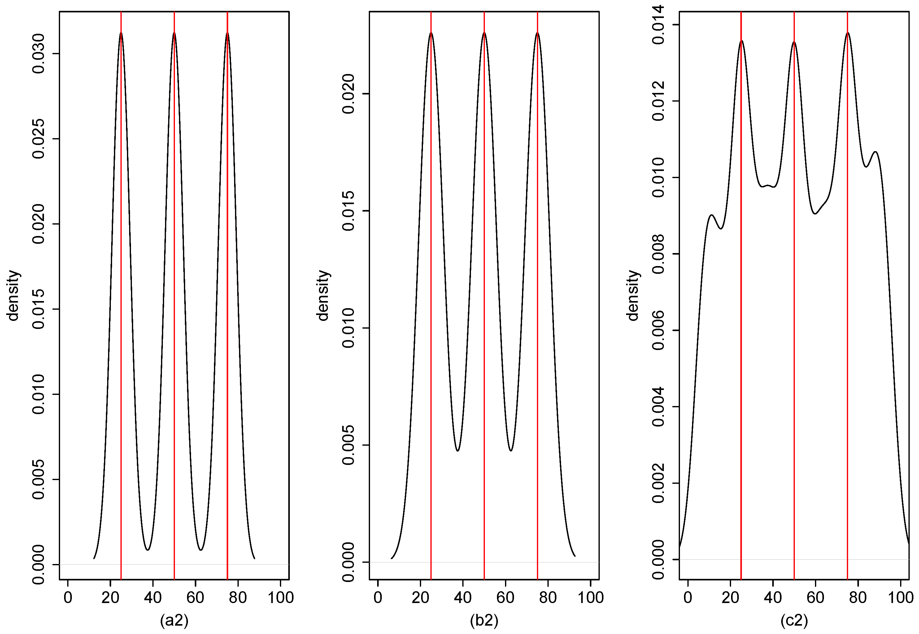
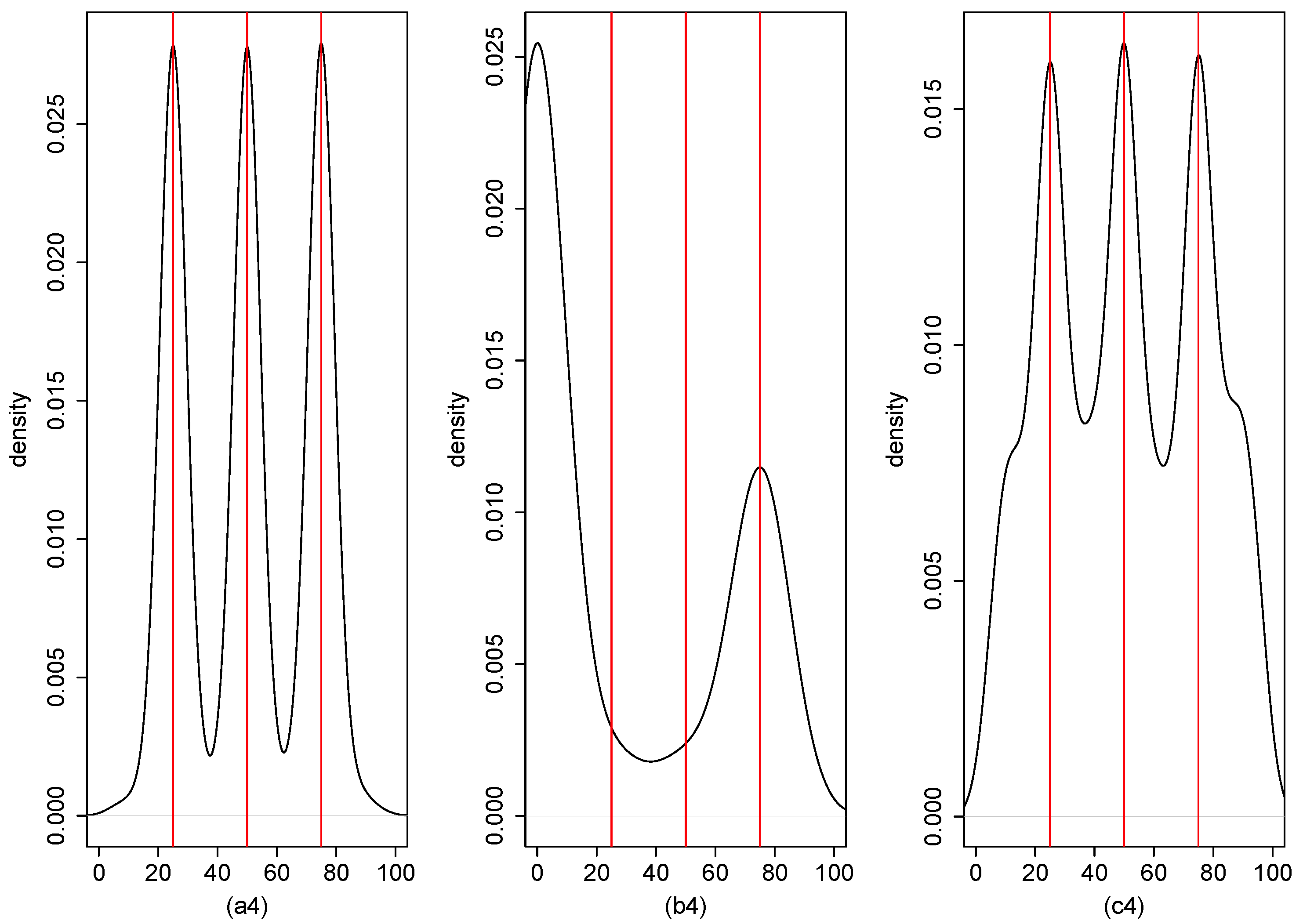
Figure 1, Figure 2, Figure 3 and Figure 4 describe the kernel density estimation of the break points obtained by SaRa-M, DCUSUM and MSSaRa when e i t are generated as (i), (ii), (iii) and (iv), respectively. From these figures, it can be seen that SaRa-M has the most distinctive aggregation feature near the true break points.
In general, based on the percentage of correct estimations of the number of break points, the mean Hausdorff distance and the location accuracy, the SaRa-M proposed in this paper performs best among the three methods, followed by the DCUSUM, and finally the mMSSaRa.

5. Empirical Example

5.1. The GDP Data

To demonstrate the suitability of the results, we used data from the World Bank Open Data (https://data.worldbank.org.cn/indicator/NY.GDP.MKTP.CD?view=chart, accessed on 21 September 2023). The original data set includes GDP data for 197 countries. However, there are some countries for which data are missing. We chose 47 countries from 1970 to 2021, including Asian countries (China, Japan, India and so on), European countries (Germany, France, Italy and so on), African countries (Nigeria, Egypt, South Africa and so on), American countries (United States, Canada, Brazil and so on), Australia and New Zealand. Missing observations were substituted by linear interpolation. Thus, the sample sizes of our analyzed data were N = 46 and T = 52. The CUSUM statistic proposed by Horvath et al. [29] was first used to test for the presence of break points, and the results showed that the null hypothesis of no break point was rejected at a 5% significance level. Using the SaRa-M proposed in this paper for break point estimation, it was found that the mean break point occurs at t = 27 (1997). The pre-break mean is
μ [ 1 , 27 ] = 1 46 × 27 i = 1 46 t = 1 27 Y i t = 0.281 × 10 12 ,
and the post-break mean is
μ [ 28 , 52 ] = 1 46 × 25 i = 1 46 t = 28 52 Y i t = 1.165 × 10 12 .
In fact, the outbreak of a financial crisis in Asia in 1997, which subsequently spread worldwide and caused enormous damage to the world economy at the time, may have contributed to the occurrence of the mean break point of the panel data.

5.2. The Real Effective Exchange Rate Index Data

In this example, we applied the modified screening sorting algorithm to investigate whether there are structural changes in the real effective exchange rate (REER) index for selected countries published by the Bank for International Settlements (BIS) (https://www.ceicdata.com.cn, accessed on 22 September 2023). We selected monthly data from the dataset for 27 countries from 2000 to 2010, including Asian countries (Japan, Korea, Singapore, Hong Kong SAR and so on), European countries (Germany, France, Italy and so on), North American countries (United States and Canada), Oceanian countries (Australia and New Zealand). The sample size of the analyzed data was N = 27 and T = 126. The CUSUM type statistic proposed by Horvath et al. [29] was first utilized to test for the presence of mean breaks, and the results showed that the original hypothesis of no breaks was rejected at the 5% significance level, i.e., there were mean breaks. The number and location of break points were then estimated using the method proposed in this paper, and the results showed that the mean break point occurs at t = 50 (February 2004). The pre-break mean is μ 1 , 50 = 97.27 , and the post-break mean is μ 51 , 126 = 100.78 .
Looking back at the world economic situation in 2004, the growth of the world economy accelerated markedly, while the sharp rise in international oil prices and the continued depreciation of the exchange rate of the United States dollar also posed a great threat to the smooth operation of the world economy. In 2004, the dollar against the euro, the yen and other major currencies experienced frequent ups and downs, an elusive trend. For example, the dollar rose against the yen from the beginning of the year’s low of 106.63 yen all the way up to the middle of May 114.88 yen in mid-May, and fell back to the end of the year 101.81 yen, a new low in 5 years, the annual decline of 4.73%. The euro, from the beginning of the year low of 1.2521 dollars, rose all the way to the end of the year of 1.3554 dollars, which was historical high, an annual increase of 7.62%.

6. Conclusions

In this paper, a modified SaRa is used to study the estimation of multiple breaks in the mean of the panel data model. Traditional multiple-sample SaRa consists of only two steps, an initial screening of possible break points by local statistics, and then a final screening of break points based on a threshold criterion. In this paper, we add an information criterion based on the above to conduct further screening. Furthermore, we prove the consistency of the break point estimators. Monte Carlo simulations show that in the case of three break points, the error term either follows a normal distribution, a GARCH process, or there is serial or cross-sectional correlation, and the modified SaRa proposed in this paper performs best compared to the double CUSUM and multiple-sample SaRa. Finally, we study the annual GDP data and the real effective exchange rate index data using the modified SaRa, and find that there exists a break point in the mean of panel data.
The method proposed in this paper is applicable to the case with breakpoints (single or multiple breakpoints), but not to the case without breakpoints. In the next step, we will propose an improved method to include the case without breakpoints.

Author Contributions

Conceptualization, F.L.; methodology, F.L., Y.X. and Z.C.; software, F.L.; validation, Y.X. and Z.C.; formal analysis, F.L. and Z.C.; investigation, F.L.; writing—original draft preparation, F.L.; writing—review and editing, F.L., Y.X. and Z.C.; visualization, F.L.; supervision, Z.C.; project administration, F.L.; funding acquisition, F.L. All authors have read and agreed to the published version of the manuscript.

Funding

This work was supported by National Nature Science Foundation of China (Program No. 12171388, 12161072, 11801438), Natural Science Basic Research Plan in Shaanxi Province of China (Program No. 2023-JC-YB-058, 2022JQ-043), Innovation Capability Support Program of Shaanxi (Program No. 2020PT-023).

Data Availability Statement

No data were used to support this study.

Acknowledgments

The authors are grateful to the Editor and reviewers for their constructive feedback and advice in the preparation of this paper.

Conflicts of Interest

The authors declare no conflict of interest.

References

  1. Csörgö, M.; Horváth, L. Limit Theorems in Change-Point Analysis; John Wiley & Sons Inc.: New York, NY, USA, 1997. [Google Scholar]
  2. Bai, J.; Perron, P. Estimating and Testing Linear Models with Multiple Structural Changes. Econometrica 1998, 66, 47–78. [Google Scholar] [CrossRef]
  3. Perron, P. Dealing with structural breaks. Palgrave Handb. Econ. 2006, 1, 278–352. [Google Scholar]
  4. Gombay, E. Change detection in autoregressive time series. J. Multivar. Anal. 2008, 99, 451–464. [Google Scholar] [CrossRef]
  5. Chen, Z.; Tian, Z. Modified procedures for change point monitoring in linear models. Math. Comput. Simulat. 2010, 81, 62–75. [Google Scholar] [CrossRef]
  6. Chen, H. Sequential change-point detection based on nearest neighbors. Ann. Stat. 2019, 47, 1381–1407. [Google Scholar] [CrossRef]
  7. Zou, C.; Yin, G.; Feng, L.; Wang, Z. Nonparametric maximum likelihood approach to multiple change-point problems. Ann. Stat. 2014, 42, 970–1002. [Google Scholar] [CrossRef]
  8. Zou, C.; Wang, G.; Li, R. Consistent selection of the number of change-points via sample-splitting. Ann. Stat. 2020, 48, 413–439. [Google Scholar] [CrossRef]
  9. Wang, Y.; Huang, G.; Yang, J.; Lai, H.; Liu, S.; Chen, C.; Xu, W. Change Point Detection with Mean Shift Based on AUC from Symmetric Sliding Windows. Symmetry 2020, 12, 599. [Google Scholar] [CrossRef]
  10. Tveten, M.; Eckley, I.A.; Fearnhead, P. Scalable change-point and anomaly detection in cross-correlated data with an application to condition monitoring. Ann. Appl. Stat. 2022, 16, 721–743. [Google Scholar] [CrossRef]
  11. Bai, J. Common breaks in means and variances for panel data. J. Econ. 2010, 157, 78–92. [Google Scholar] [CrossRef]
  12. Kim, D. Estimating a common deterministic time trend break in large panels with cross sectional dependence. J. Econ. 2011, 164, 310–330. [Google Scholar] [CrossRef]
  13. Kim, D. Common local breaks in time trends for large panels. Econ. J. 2014, 17, 301–337. [Google Scholar]
  14. Peštová, B.; Pešta, M. Testing structural changes in panel data with small fixed panel size and bootstrap. Metrika 2015, 78, 665–689. [Google Scholar] [CrossRef]
  15. Baltagi, B.H.; Feng, Q.; Kao, C. Estimation of heterogeneous panels with structural breaks. J. Econ. 2016, 191, 176–195. [Google Scholar] [CrossRef]
  16. Xu, M.; Zhong, P.; Wang, W. Detecting variance change-points for blocked time series and dependent panel data. J. Bus. Econ. Stat. 2016, 34, 213–226. [Google Scholar] [CrossRef]
  17. Horváth, L.; Hušková, M.; Rice, G.; Wang, J. Asymptotic properties of the CUSUM estimator for the time of change in linear panel data models. Econ. Theor. 2017, 33, 366–412. [Google Scholar] [CrossRef]
  18. Lumsdaine, R.L.; Okui, R.; Wang, W. Estimation of panel group structure models with structural breaks in group memberships and coefficients. J. Econ. 2023, 233, 45–65. [Google Scholar] [CrossRef]
  19. Feng, Q.; Kao, C.; Lazarova, S. Estimation of Change Points in Panels; Working Paper; Syracuse University: New York, NY, USA, 2009. [Google Scholar]
  20. Li, D.; Qian, J.; Su, L. Panel data models with interactive fixed effects and multiple structural breaks. J. Am. Stat. Assoc. 2016, 111, 1804–1819. [Google Scholar] [CrossRef]
  21. Qian, J.; Su, L. Shrinkage estimation of common breaks in panel data models via adaptive group fused lasso. J. Econ. 2016, 191, 86–109. [Google Scholar] [CrossRef]
  22. Okui, R.; Wang, W. Heterogeneous structural breaks in panel data models. J. Econ. 2020, 220, 447–473. [Google Scholar]
  23. Kaddoura, Y.; Westerlund, J. Estimation of panel data models with random interactive effects and multiple structural breaks when T is Fixed. J. Bus. Econ. Stat. 2022, 41, 1–38. [Google Scholar] [CrossRef]
  24. Cho, H. Change-point detection in panel data via double CUSUM statistic. Electron. J. Stat. 2016, 10, 2000–2038. [Google Scholar] [CrossRef]
  25. Song, C.; Min, X.; Zhang, H. The screening and ranking algorithm for change-points detection in multiple samples. Ann. Appl. Stat. 2016, 10, 2102–2129. [Google Scholar] [CrossRef] [PubMed]
  26. Niu, Y.S.; Zhang, H. The screening and ranking algorithm to detect DNA copy number variations. Ann. Appl. Stat. 2012, 6, 1306–1326. [Google Scholar] [CrossRef]
  27. Hao, N.; Niu, Y.S.; Zhang, H. Multiple change-point detection via a screening and ranking algorithm. Statist. Sin. 2013, 23, 1553–1572. [Google Scholar] [CrossRef]
  28. Xiao, F.; Min, X.; Zhange, H. Modified screening and ranking algorithm for copy number variation detection. Bioinformatics 2015, 31, 1341–1348. [Google Scholar] [CrossRef]
  29. Horváth, L.; Hušková, M. Change-point detection in panel data. J. Time Ser. Anal. 2012, 33, 631–648. [Google Scholar] [CrossRef]
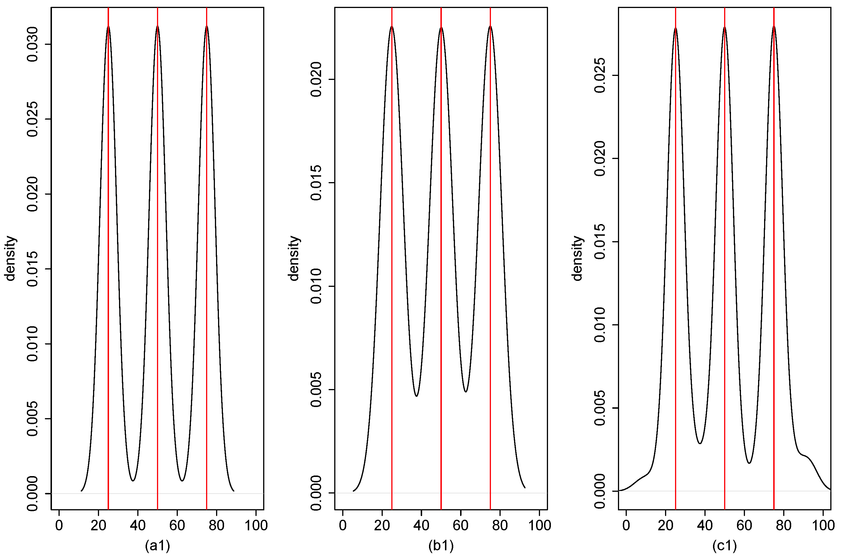
Figure 1. When e i t are generated as (i), the kernel density estimation of the three break points ( τ 1 = 25 , τ 2 = 50 , τ 3 = 75 ) obtained by SaRa-M (a1), DCUSUM (b1) and MSSaRa (c1), respectively, is shown. The sample size N = T = 100 .
Symmetry 15 01890 g001
Figure 2. When e i t are generated as (ii), the kernel density estimation of the three break points ( τ 1 = 25 , τ 2 = 50 , τ 3 = 75 ) obtained by SaRa-M (a2), DCUSUM (b2) and MSSaRa (c2) respectively, is shown. The sample size N = T = 100 .
Symmetry 15 01890 g002
Figure 3. When e i t are generated as (iii), the kernel density estimation of the three break points ( τ 1 = 25 , τ 2 = 50 , τ 3 = 75 ) obtained by SaRa-M (a3), DCUSUM (b3) and MSSaRa (c3) respectively, is shown. The sample size N = T = 100 .
Symmetry 15 01890 g003
Figure 4. When e i t are generated as (iv), the kernel density estimation of the three break points ( τ 1 = 25 , τ 2 = 50 , τ 3 = 75 ) obtained by SaRa-M (a4), DCUSUM (b4) and MSSaRa (c4) respectively, is shown. The sample size N = T = 100 .
Symmetry 15 01890 g004
Table 1. The estimation results of SaRa-M, DCUSUM and MSSaRa when e i t are generated as (i) in case of a single break point and three break points.
Single Break PointThree Break Points
N/T J ^ < 1 J ^ = 1 J ^ > 1MHDLocation Accuracy J ^ < 3 J ^ = 3 J ^ > 3MHDLocation Accuracy
τ 1 τ 1 τ 2 τ 3
SaRa-M50/50010000.416996.293.801.752949499.8
50/100010000.44699.6010000.336100100100
100/50010000.122100010000.062100100100
100/100010000.122100010000.056100100100
DCUSUM50/50099.50.50.3159965.534.5016.29136.53598.5
50/100099.50.50.21100010000.599.599.5100
100/50010000.0710031.568.508.05568.568.5100
100/100010000.035100010000.16100100100
MSSaRa50/500.8972.20.74497.8392.84.20.96610097.698.8
50/1001.88117.24.79896.8077.622.42.812100100100
100/50098.41.60.34499.8097.62.40.212100100100
100/100083174.968100074.425.62.974100100100
Table 2. The estimation results of SaRa-M, DCUSUM and MSSaRa when e i t are generated as (ii) in case of a single break point and three break points.
Single Break PointThree Break Points
N/T J ^ < 1 J ^ = 1 J ^ > 1 MHDLocation Accuracy J ^ < 3 J ^ = 3 J ^ > 3 MHDLocation Accuracy
τ 1 τ 1 τ 2 τ 3
SaRa-M50/50010000.07499.80.299.800.0610010099.6
50/100010000.09299.8010000.042100100100
100/50010000.02499.8010000.002100100100
100/100010000.01100010000.01100100100
DCUSUM50/5009910.135100158503.98585100
50/10009910.15100010000.04100100100
100/50010000100010000.01100100100
100/100010000100010000.02100100100
MSSaRa50/500.294.65.20.82299.2056.443.62.9399.9100100
50/1000.68118.44.9998.8024.575.59.38199.9100100
100/50070.829.24.098100034.265.84.50199.999.9100
100/100015.384.725.63799.80010017.058100100100
Table 3. The estimation results of SaRa-M, DCUSUM and MSSaRa when e i t are generated as (iii) in case of a single break point and three break points.
Single Break PointThree Break Points
N/T J ^ < 1 J ^ = 1 J ^ > 1 MHDLocation Accuracy J ^ < 3 J ^ = 3 J ^ > 3 MHDLocation Accuracy
τ 1 τ 1 τ 2 τ 3
SaRa-M50/50082183.71879.2257505.4368381.491.8
50/100010001.60689.26139029.3543.243.693.2
100/50081192.86491.80.493.46.20.7899.698.299.6
100/100098.21.81.23895.80.299.60.20.58699.699.299.6
DCUSUM50/50198101.253851000022.48512.517.565.5
50/10009731.6692.56337031.67335.534.593
100/5019900.57694.5991023.05211.511.583.5
100/100095.54.51.3998.520.579.5010.78787799
MSSaRa50/50059.240.86.91672.41.245.453.44.32898.895.897.8
50/1000010035.62881.20010017.56897.29897.6
100/50067.632.45.254890.458.241.43.22299.498.899.6
100/1000010035.61900010017.67810099.899.8
Table 4. The estimation results of SaRa-M, DCUSUM and MSSaRa when e i t are generated as (iv) in case of a single break point and three break points.
Single Break PointThree Break Points
N/T J ^ < 1 J ^ = 1 J ^ > 1 MHDLocation Accuracy J ^ < 3 J ^ = 3 J ^ > 3 MHDLocation Accuracy
τ 1 τ 1 τ 2 τ 3
SaRa-M50/50085.414.63.57482.633.865.218.2970.470.491.2
50/100098.21.82.2669015.683.21.29.83279.48093.8
100/50061.838.25.9686.66.884.48.83.06293.890.497.2
100/100089114.25691.40.491.87.83.1595.496.496.6
DCUSUM50/50534702.319831000023.846481349
50/10099012.52786982043.383132275
100/50495102.157751000020.304193145
100/10009552.22958713039.892202185
MSSaRa50/502.382.515.23.95376.20.275.923.91.48999.499.799.3
50/1001.123.875.123.48179.50.17.192.812.9419594.495.1
100/500.18019.94.35280.53.67026.43.29296.793.796.5
100/100099128.90893.402.597.514.15597.39796.2
Disclaimer/Publisher’s Note: The statements, opinions and data contained in all publications are solely those of the individual author(s) and contributor(s) and not of MDPI and/or the editor(s). MDPI and/or the editor(s) disclaim responsibility for any injury to people or property resulting from any ideas, methods, instructions or products referred to in the content.