Article

Learning by Autonomous Manifold Deformation with an Intrinsic Deforming Field

by
Xiaodong Zhuang
1,* and
Nikos Mastorakis
2
1
Electronics Information College, Qingdao University, Qingdao 266071, China
2
Department of Industrial Engineering, Technical University of Sofia, Bulevard Sveti Kliment Ohridski 8, 1000 Sofia, Bulgaria
*
Author to whom correspondence should be addressed.
Symmetry 2023, 15(11), 1995; https://doi.org/10.3390/sym15111995
Submission received: 25 September 2023 / Revised: 23 October 2023 / Accepted: 27 October 2023 / Published: 29 October 2023

Abstract

:
A self-organized geometric model is proposed for data dimension reduction to improve the robustness of manifold learning. In the model, a novel mechanism for dimension reduction is presented by the autonomous deforming of data manifolds. The autonomous deforming vector field is proposed to guide the deformation of the data manifold. The flattening of the data manifold is achieved as an emergent behavior under the virtual elastic and repulsive interaction between the data points. The manifold’s topological structure is preserved when it evolves to the shape of lower dimension. The soft neighborhood is proposed to overcome the uneven sampling and neighbor point misjudging problems. The simulation experiment results of data sets prove its effectiveness and also indicate that implicit features of data sets can be revealed. In the comparison experiments, the proposed method shows its advantage in robustness.

1. Introduction

Dimension reduction (DR) is an indispensable technique to face the challenge of dramatically increasing data amounts in data analysis [1,2,3,4,5,6]. Non-linear DR is a current research focus, where manifold learning is one of the main research topics [5,6]. In addition to the ability of unsupervised non-linear dimension reduction and feature extraction, manifold learning provides a geometric viewpoint for modern data analysis, where the data set contains the samples from the data manifold. Moreover, research has proved that the visual information represented in the neural system can also be modeled in a manifold-based way [7,8,9]. Therefore, the manifold-based model has attracted extensive research attention since the publication of isometric mapping (Isomap) and local linear embedding (LLE). Other methods have been proposed such as Laplacian eigenmaps (LE) and Hessian Laplacian eigenmaps, maximum variance unfolding (MVU) and landmark maximum variance unfolding, Riemannian manifold learning, locally linear coordination, stochastic neighbor embedding and t-distributed stochastic neighbor embedding (t-SNE), local tangent space alignment (LTSA), locality preserving projection (LPP), etc. [10,11,12,13,14,15,16,17,18,19,20]. Some methods have several variations. Moreover, some frameworks of manifold learning have also been proposed to classify manifold learning methods, such as graph embedding framework, patch alignment framework, and kernel framework [17,18,19,20].
Although impressive experimental results have been achieved by manifold learning, some common problems still exist, such as uneven data sampling, small sample size, and out-of-sample problem [20,21,22,23,24,25]. It has also been proposed that current manifold learning models may fail on those data manifolds with extremely high dimension or high local curvature [20,21,22,23]. The goal of manifold learning is to generate a meaningful, smooth, and consistent mapping from the original data set to a low-dimensional representation. Manifold learning usually builds the mapping by some mathematical optimization method in which the preservation of a local neighborhood structure is the main constraint. For example, multi-dimensional scaling is used in Isomap, semi-definite programming is used in MVU, a gradient descent algorithm is used in t-SNE, etc. The accuracy of local neighborhood constraint is one key determining the effectiveness of the optimization result. The learning significantly depends on the selection of neighborhood points as the first step in the learning algorithm. In practical applications, the difficulty of neighbor point selection as well as intrinsic dimension estimation are commonly encountered [20,21,22,23,24,25]. The learning may be made invalid because the practical data sets usually do not satisfy the requirement of dense and uniform sampling on the manifold, which becomes the bottleneck for the practical application of manifold learning methods.
To overcome these, for this paper, topological deformation learning was proposed to improve the robustness by overcoming the uneven sampling and neighbor point misjudging. Inspired by a self-evolutionary and self-adaptive natural mechanism, the method implements the DR process as the geometric flattening of the manifold in Rn. The natural intelligent mechanism is usually self-organized with an emergent behavior of a swarm with simple individuals (such as ant colony, bee colony, neuron systems, etc.) [26,27,28]. The proposed method implemented an emergent behavior mechanism in which the data manifold (in a discrete form) deformed autonomously by the virtual interaction between the data points. The DR result could be naturally derived from the flattened manifold. And the intrinsic dimension of the manifold was naturally indicated in the deforming result. Moreover, a “soft neighborhood” of the data point was presented to overcome the difficulties caused by neighbor point misjudging and non-uniform sampling. Compared with typical and improved approaches, the experimental results proved the effectiveness and robustness of the proposed model, which presented a new category of manifold learning method.

2. Dimension Reduction by Autonomous Deformation of Data Manifolds

Current learning methods for DR usually build a mapping from the original data into a low-dimensional space while keeping local properties as unchanged as possible (i.e., the distance or angles between neighbor data points). Such local constraints within the neighbor area are sensitive to perturbation such as noise in data or computation errors. This may greatly affect the validity of the DR result [21,22,23].
Geometrically, the data points are distributed on (or close to) the ideal data manifold, which facilitates the application of topology tools. Topological deformation is continuous and preserves the basic geometric properties (i.e., topological properties). A new DR model is inspired by analyzing the inverse process of flattening, i.e., how a flat manifold is changed to a geometry of a more complex shape in the embedded space Rn. For intuitive comprehension, consider the following cases. Folding or curling a piece of paper will make the points on the paper leave the initial plane and move to another position in R3. In another case, making a flat elastic film uneven or cratering can also cause some points to move to their new position in R3. In the first case, in the folding or curling process, points that were originally far away may come close. To restore the original shape, the distance between such points should be increased as large as possible while preserving the distance between those neighbor points that are close enough (otherwise the paper will be torn). For the second case, because the geometric structure in the convex or concave parts was already non-linear, optimal DR results may be obtained by proper “stretching”. Overall consideration of these cases inspires a reasonable way of DR by “flattening”, in which the distances between points are increased as much as possible, while properly preserving the distance between those points that were originally close enough. A similar idea appeared in the maximum variance unfolding (MVU) method, in which the DR is achieved in a traditional optimization framework.
The proposed model is based on a geometric interpretation of dimension reduction as flattening the data manifold. In topological deformation learning, the manifold geometry flattens autonomously as a deforming geometric object in the embedded space, which is guided by an intrinsic deforming vector field defined on the manifold. The deforming vector field is based on two different virtual interactions between data points. By the proper balance between the virtual elastic and repulsive interactions, the manifold can flatten autonomously as an emergence effect. Especially, the soft neighborhood is proposed to overcome the problem of non-even sampling on the manifold, which may invalidate traditional methods including MVU. By the emergent behavior of the interacting manifold points, the manifold can autonomously deform (or self-evolve) and the DR results can naturally be achieved by the deforming result.

2.1. The Soft Neighborhood of Data Points

Useful information and intrinsic features are implicitly contained in the data manifold’s topological structure. Preserving the topological structure is a basic constraint for DR methods. The discrete data points are considered samplings from the data manifold, and the data manifold’s topological structure is expressed by the neighborhood relationship between data points. In manifold learning, it is usually the first step to search the neighbors for each data point. Current methods include fixed neighborhood radius or fixed number of neighbor points, which are suitable for the uniform and dense sampling of the manifold. However, practical data sets may have a limited number of data points, and the sampling is often non-uniform. This will cause some misjudgment of neighbor points, which may invalidate the learning. For the k nearest neighbor points, if k is large, some non-neighbor points will be included, which will cause a “short-circuit edge”. To overcome this problem, the “soft neighborhood” method was proposed.
Suppose the data point set is {p1, p2, …, pn} where n is the number of total data points. For each point pi on the initial manifold (i.e., the one before deforming), find the m nearest points as its neighbor set Ni = {q1, q2, …, qm}. The value of m can be properly large so that no true neighbor point is missed. To overcome the “short-circuit edge” problem, the neighbor degree is defined. Let dij denote the distance between pi and qj. Let dmini denote the minimum value in {dij}, j = 1, 2, …, m. The neighbor degree for pi’s neighbor set is:
N D i j = d m i n i d i j   j = 1 , 2 , , m ;   i = 1 , 2 , , n
where NDij is the neighbor degree of qj to pi. There is 0 < N D i j 1.0 , which is similar to the degree of membership in a fuzzy set [29]. If qj is a non-neighbor point (a misjudged one), the NDij value will be very small. Therefore, NDij quantitatively expresses to what degree qj is a true neighbor point of pi. The proper use of NDij in the DR technique can eliminate the severe interference of the “short-circuit edge”. In the proposed model, NDij has a key role in the definition of interactions between data points. A more precise expression of pi’s soft neighborhood is:
S N i = { ( q j , N D i j ) }   j = 1 , 2 , , m ;   i = 1 , 2 , , n
where qj belongs to the m nearest points and NDij is the neighbor degree of qj to pi.

2.2. Intrinsic Deforming Vector Field with Flattening Effect

To achieve dimension reduction by manifold deformation, two virtual interactions between data points were proposed to guide the autonomous deforming process: the repulsive interaction and the elastic interaction.
The repulsive interaction vector from the data point pj to pi was proposed as:
V i j r =   ( 1.0 N D i j ) · ( p i p j ) d i j   p j N i   p i p j d i j   o t h e r w i s e  
where p i and p j are the position vectors in Rn for the data points pi and pj, dij is the distance between pi and pj, and NDij is the neighboring degree of pj to pi. If pi moves along the direction of the vector ( p i p j ) in Rn, it will move away from pj. Therefore, the vector defined in Equation (3) has a repulsive effect between pi and pj.
On the other hand, the elastic interaction vector between pi and pj was proposed as:
V i j e =   N D i j · ( d i j 0 d i j ) · ( p i p j ) d i j   p j N i   0   o t h e r w i s e  
where d i j 0 is the Euclidean distance between pi and pj on the original manifold (before deforming) and dij is the distance between pi and pj in the deforming process, which changes dynamically according to the shape of the deforming manifold. Correspondingly, the interaction vector defined in Equation (4) will also alter according to the manifold shape. For each point pi, this elastic interaction only exists for the points in its soft neighborhood NSi. For a point pj in NSi, if pj goes away from pi in the deforming manifold (i.e., the current distance dij is larger than the original value d i j 0 ), it will attract pi; otherwise, it will repel pi. This is an elastic effect preserving the distance between the neighbor points (i.e., keeping the neighborhood structure in the deforming process).
In Equations (3) and (4), NDij properly weights the two different interactions between the data points in a soft neighborhood. In case there is a “short-circuit edge”, the actual non-neighbor point pj will have a very small NDij value (i.e., close to zero). And the interaction between pj and pi is mainly repulsive, just similar to those non-neighbor points. Therefore, the problem caused by the “short-circuit edge” can be solved adaptively.
The total interaction effect on pi from all the other data points is defined as the weighted sum of the above two kinds of interactions:
V i = α 1 · j = 1 j i N V i j r + α 2 · j = 1 j i N V i j e   ( α 1 > 0 ,   α 2 > 0 , α 1 + α 2 = 1.0 )
where N is the number of data points; α1 and α2 are two weight coefficients that balance the two kinds of interactions, which satisfy α1 > 0, α2 > 0, and α1 + α2 = 1; and V i is defined as the deforming vector on pi, according to which each point on the manifold changes its location in the deforming process. Because V i is completely determined by the current shape of the manifold itself, this vector field is intrinsic. If each pi moves according to V i (i.e., takes V i as the moving direction), one step of manifold deforming will take place. If such a step repeats, the deformation of the data manifold will proceed step by step. Due to the intrinsic nature of the deforming vector field, the deformation is a kind of self-evolution of the manifold. Moreover, the deforming process will converge to a result of a flattened shape in Rn, based on which the dimension reduction result can be naturally derived.

2.3. The Manifold Deformation Learning Algorithm

Based on the definition of deforming vector field, the manifold deformation learning algorithm was proposed as follows.
Step 1:
Compute the Euclidean distance dij between each pair of data points in the original data set.
Step 2:
For each data point pi, find the k nearest neighbor points as the members of its soft neighborhood point set.
Step 3:
For each data point pi, compute the neighbor degree NDij of each point in its soft neighborhood set.
Step 4:
The counter of the deforming steps C is initialized to zero.
Step 5:
For each data point pi, compute the displacement vector V i according to Equation (5) ( V i is determined by p i s current position and the current manifold shape in Rn).
Step 6:
For each data point pi, update p i s position according to V i .
Step 7:
Increase C by 1.
Step 8:
Check the termination condition. If the sum of V i for all the points is smaller than a threshold ε or C reaches a given value Cmax, go to Step 9. Otherwise, return to Step 5.
Step 9:
Carry out principal component analysis (PCA) on the deformed manifold to obtain the final dimension reduction result (the number of principal components is taken as the estimated intrinsic dimension of the manifold, and the low-dimension coordinates of each data point pi are computed by the projection onto the principal component vectors).
In the above algorithm, the data manifold first flattens in Rn. Then, the manifold intrinsic dimension is estimated by PCA. Simultaneously, the DR result is obtained after the manifold has already been fairly flattened. The proposed model belongs to global learning considering the definition of V i j r and the progressive (or stepwise) spread of local deformation to distant areas on the manifold. Although the elastic interaction is defined within a soft neighborhood of a point, based on the connectivity of neighboring points in the manifold topology, this local interaction will gradually affect the points far away. The local–global interaction of data points results in the autonomous deforming of the manifold, or its self-evolution. Although PCA is used in the last step of the algorithm, the method is non-linear due to the deforming process.

3. Simulation Study on Data Sets

The proposed model was implemented by a programming simulation. In the preliminary experiments, it was discovered that the values of α1 and α2 had an obvious impact on the results. If α1 was much larger, the repulsion between data points would be very strong. The manifold would be rapidly flattened and also stretched, but the distance between neighbor points could hardly be preserved. (Interestingly, in this case, the deforming still reached a balanced state, in which the elastic interaction between neighbor points became a strong attraction to counteract the repulsion between points.) On the contrary, if α2 was much larger, the elastic interaction between neighbor points would be strong, which could preserve the neighbor distances well, but the deforming of the manifold would become very slow. The dynamic alternation of α1 and α2 was proposed to overcome this. In the deforming process, we let α1 rise and fall periodically, but kept α2 constant. In this way, the repulsion prevailed over the elastic interaction for some time, and then the elastic interaction in turn became dominant. Correspondingly, the deforming process alternated periodically between the two stages of “flattening” and “restoring neighbor distance”. The updating of α1 and α2 was implemented in Step 5 before the calculation of the displacement vector.

3.1. Simulation Study on Test Data Sets

Experiments were performed on typical surfaces in R3. Some of the results are shown for the S-surface and the Gaussian surface (corresponding to the cases of curling and convex or concave shapes, respectively).
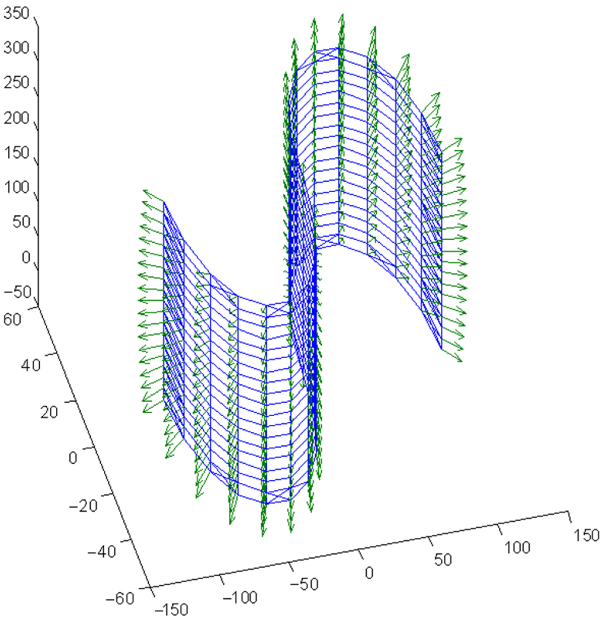
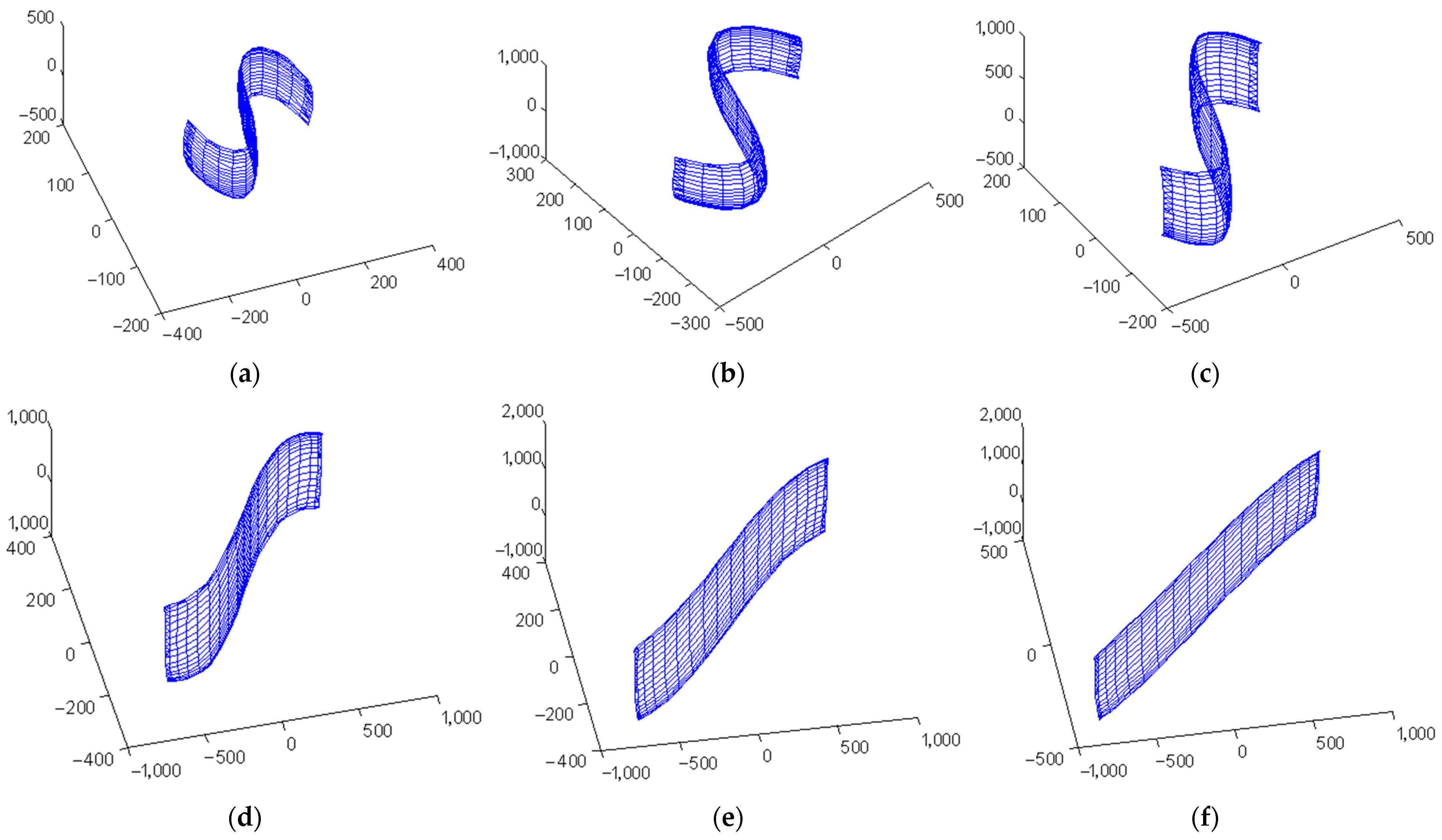
Figure 1 shows the mesh of the S-surface, which had 360 data points. The edges represent the neighboring relationship between the data points. Figure 2 shows the displacement vectors on the initial data mesh in 3D, which were calculated according to Equation (5). It is clear that these vector directions represented by the arrows had the effect of stretching the surface in a flattening tendency. Intermediate results were recorded in the experiment, which are shown in Figure 3 as a demonstration of the deformation process.
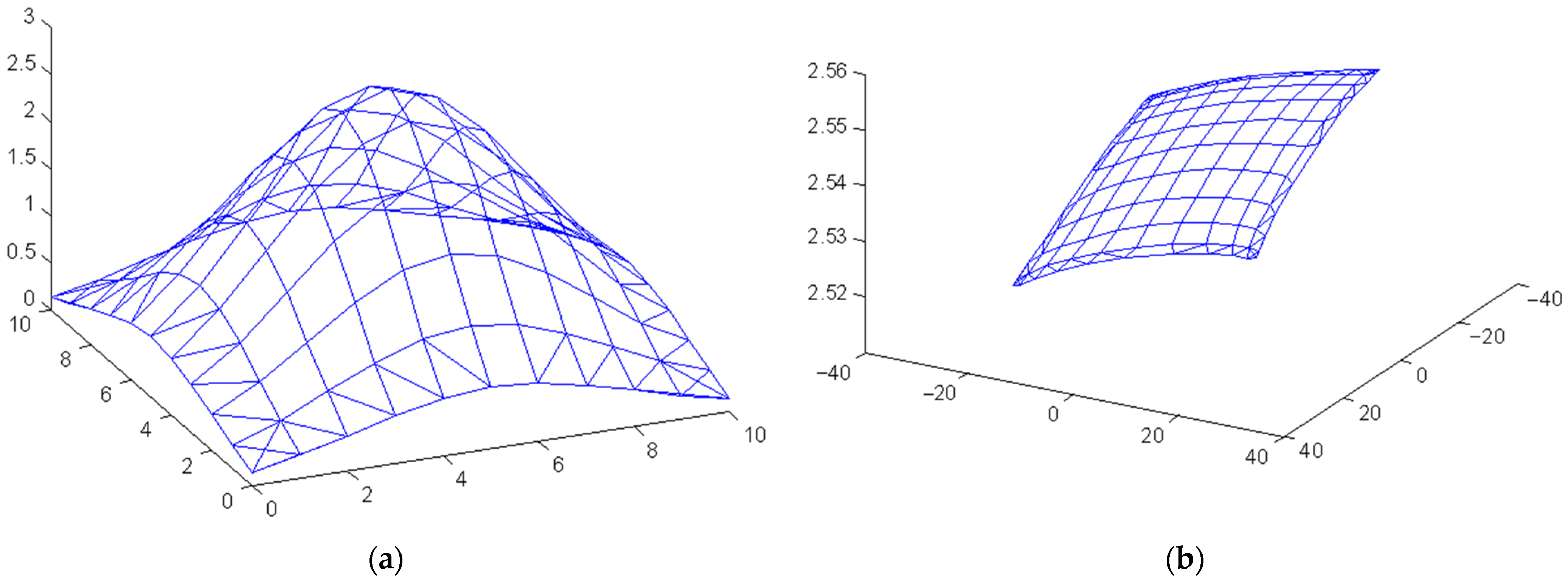
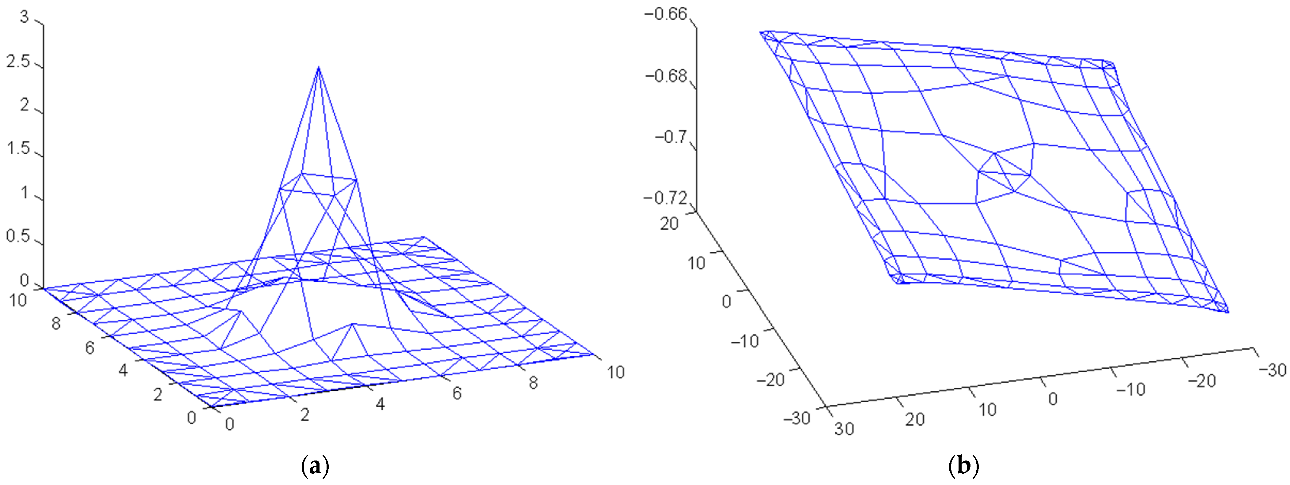
The experimental results for the Gaussian surfaces are shown in Figure 4, Figure 5, Figure 6 and Figure 7. Figure 4a and Figure 6a show two Gaussian surfaces with different variance values, which had 120 data points, respectively. Figure 6a has a smaller variance value; therefore, the shape appears much sharper. Figure 4 and Figure 6b are the deforming results in R3, respectively. Figure 5 and Figure 7 show the final DR results. The intrinsic dimension of the data sets was revealed as 2. The topology structure of the data set was based on the neighborhood relationship of data points. The DR results consisted of the nodes representing data points and the edges representing the neighborhood relationship. Each node is labeled with the number of its corresponding data point. Due to the non-linear property of the Gaussian surface, the dimension reduction results were not evenly distributed. However, the distance between neighbor points was as relatively preserved as possible.

3.2. Simulation Study on Practical Data Sets

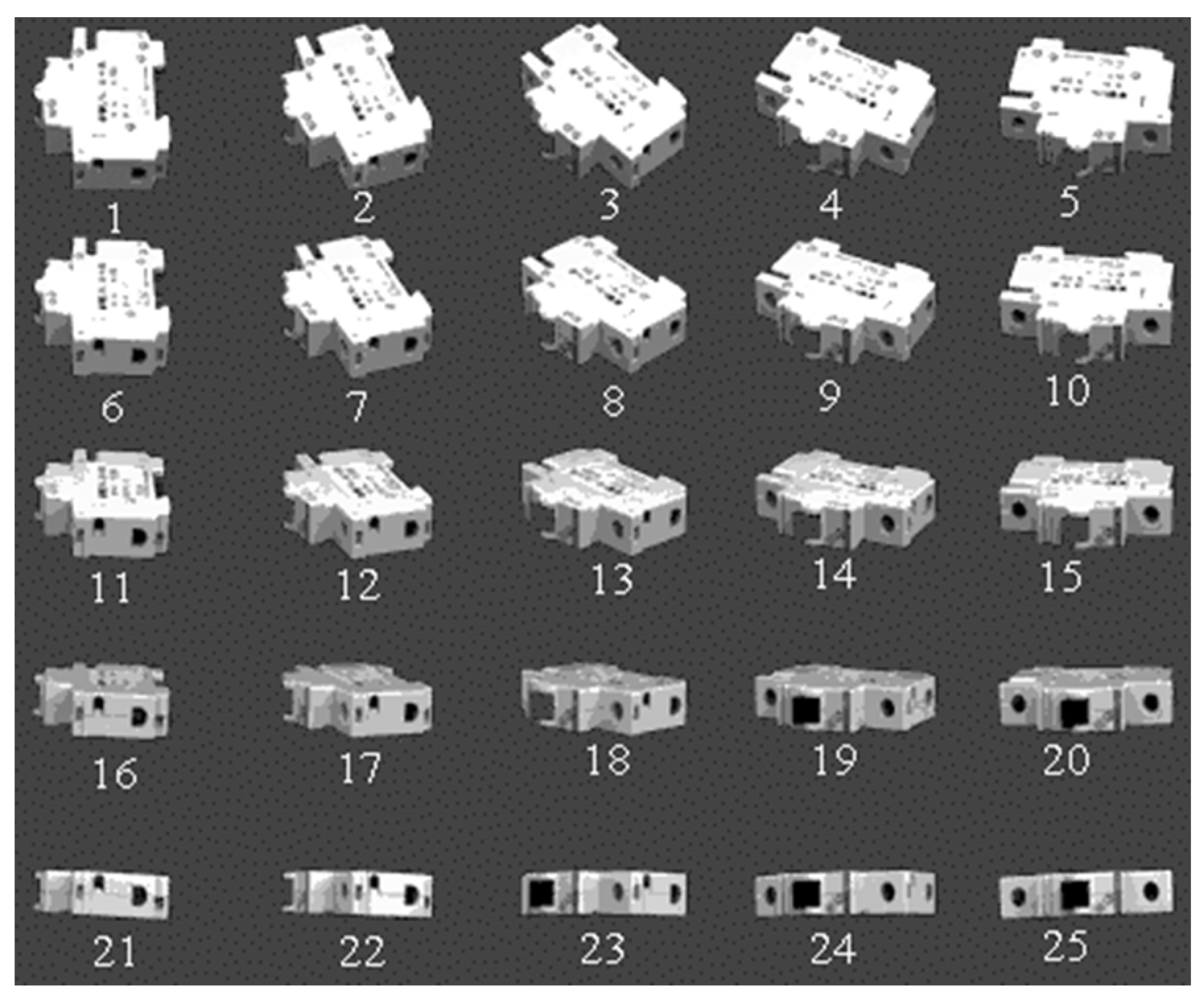
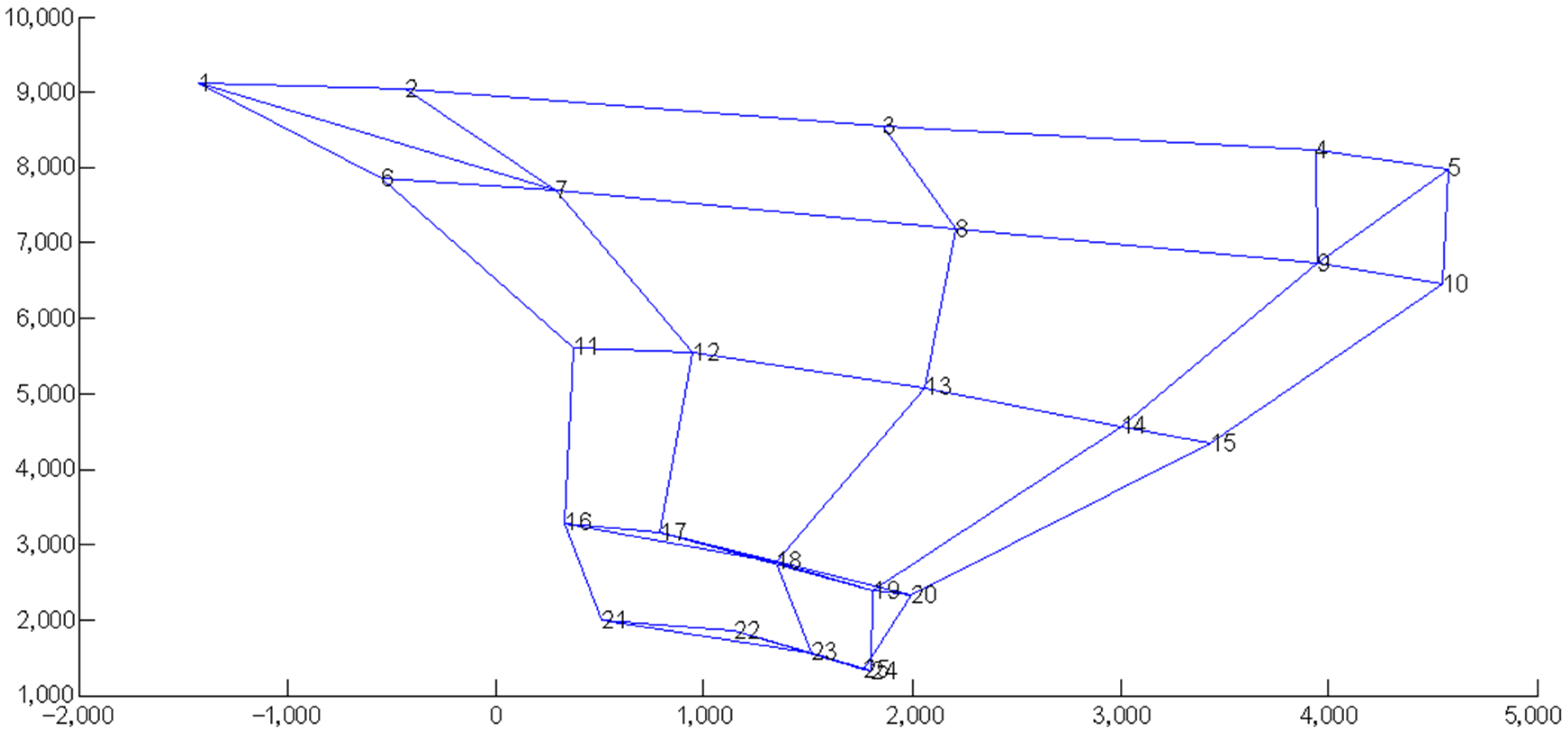
Figure 8 and Figure 9 show the DR result of the auto fuse image set from the “Object Pose Estimation Database” [30,31]. This image set was captured under the viewpoints with horizontal and vertical changes. Figure 8 shows the data set with a number assigned to each image. The dimension reduction result is shown in Figure 9 with several nodes and edges. In the DR result, the intrinsic dimension was estimated as 2. Each node in Figure 9 corresponds to an image with the same number in Figure 8. The pairs of neighbor data points in the original data set are represented by the pairs of nodes connected by the edges in Figure 9. The two different dimensions in Figure 9 have meaningful interpretations, respectively. The x-axis corresponds to the change in the horizontal viewpoint. The y-axis corresponds to the change in the vertical viewpoint. The nodes at the lower right area of the grid in Figure 9 are much closer because the method preserved the distance between neighbor points in manifold deformation, and those distances were relatively small in the original data set.
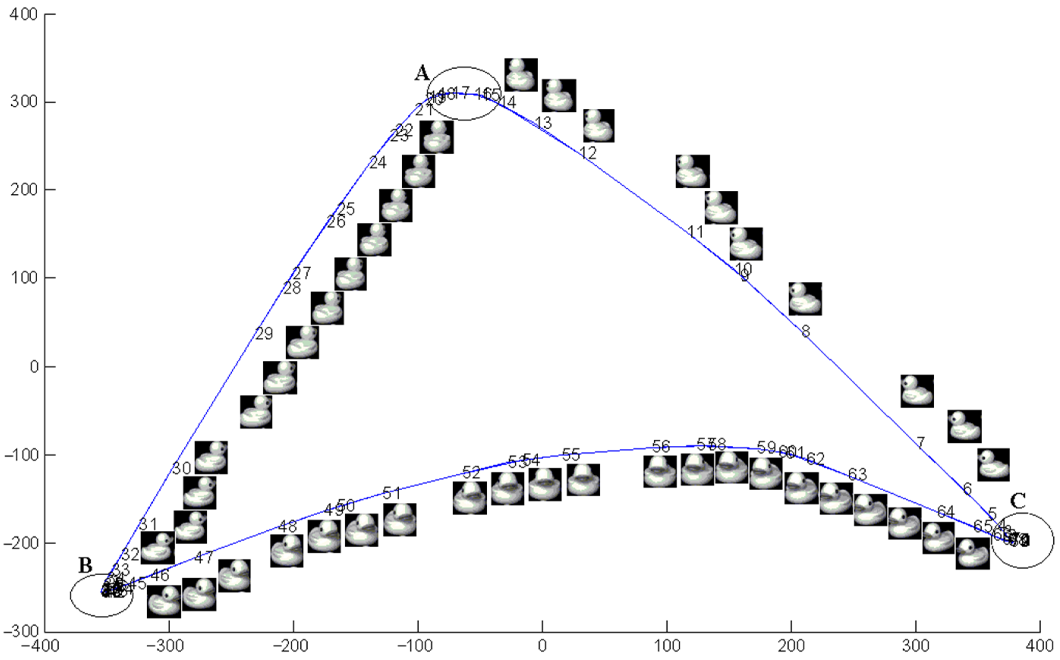
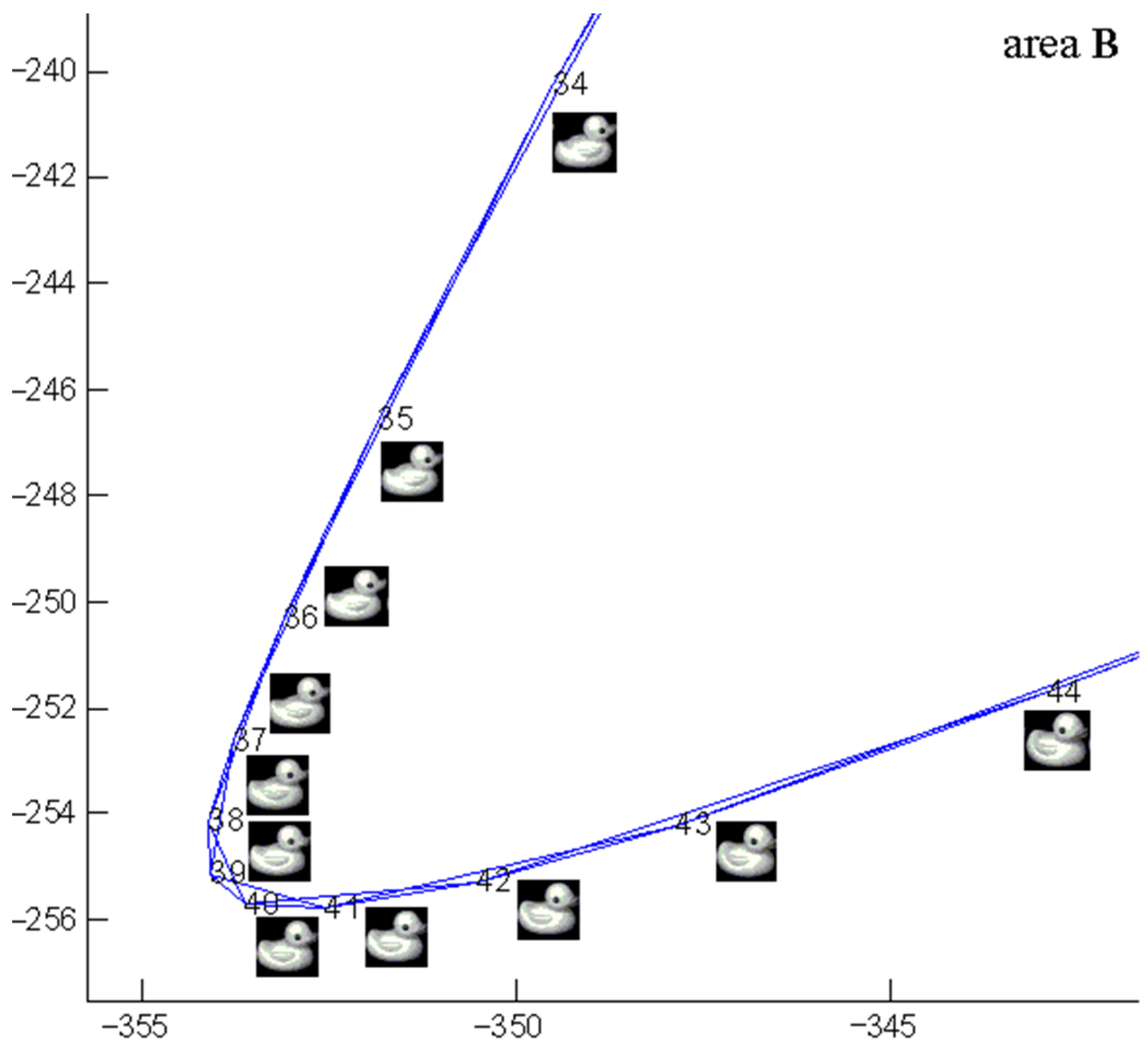
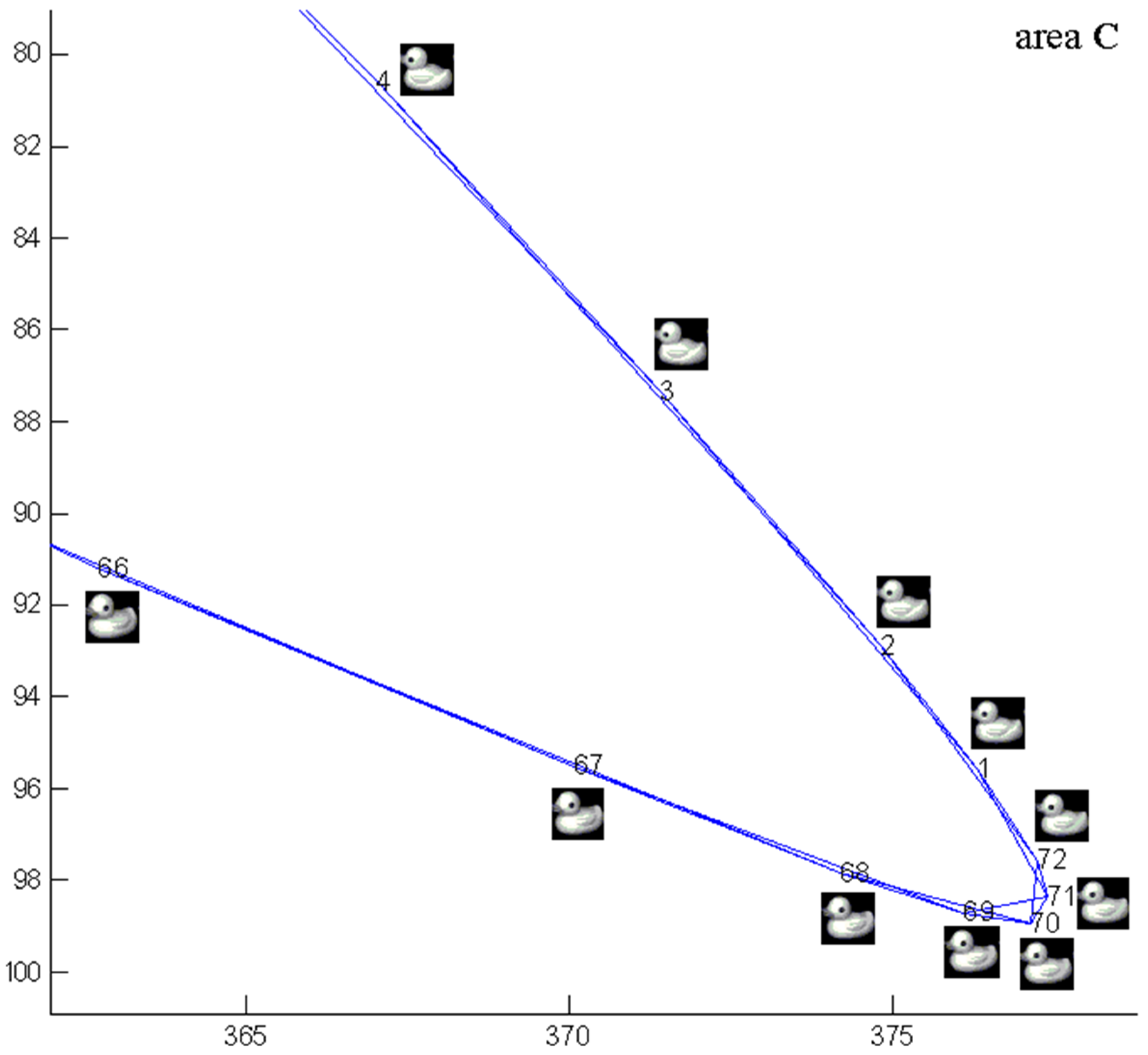
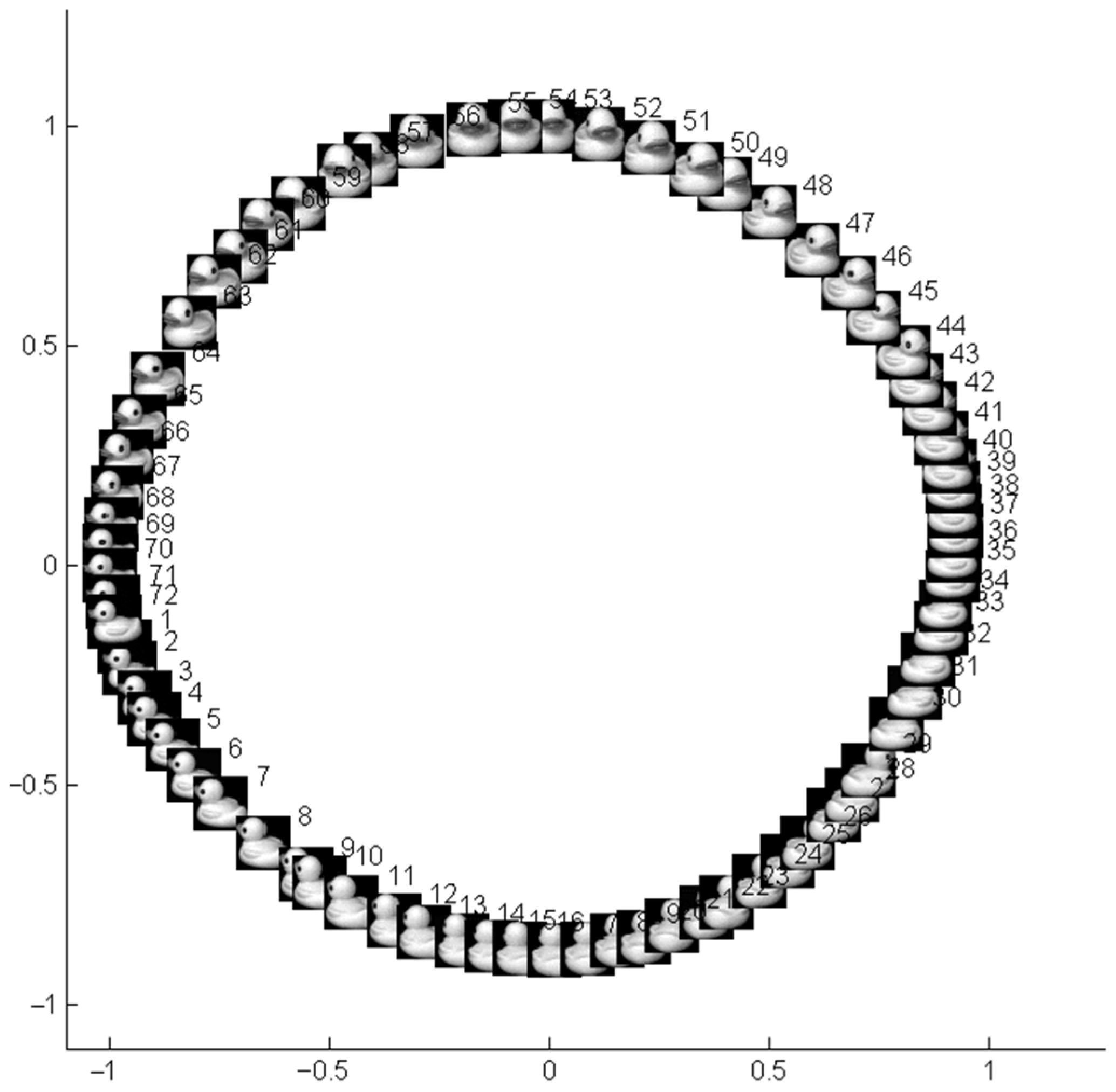
Figure 10 shows a group of image sequences from the “Columbia Object Image Library (COIL-20)”, which is captured for rotating and simultaneously resizing objects [32,33]. In Figure 10, the toy rotates 360 degrees, together with a simultaneous size variation. The result of the dimension reduction is shown in Figure 11, where each node is labeled with a corresponding image number. The toy images are also displayed near their corresponding nodes. Figure 11 shows a closed curve representing the rotating angle variation from 0 to 360 degrees. The x-axis corresponds to the left–right rotating angle. The y-axis is related to the size factor. In Figure 11, the points are very close at the top, lower left, and lower right areas on the curve (indicated as areas A, B, and C in the figure). These three areas are shown in Figure 12, Figure 13 and Figure 14 in more detail. The variation in the images along the curve in Figure 11 is consistent with the rotating process and also consistent with the resizing process. Therefore, the topology structure of this data set can be seen in Figure 11.
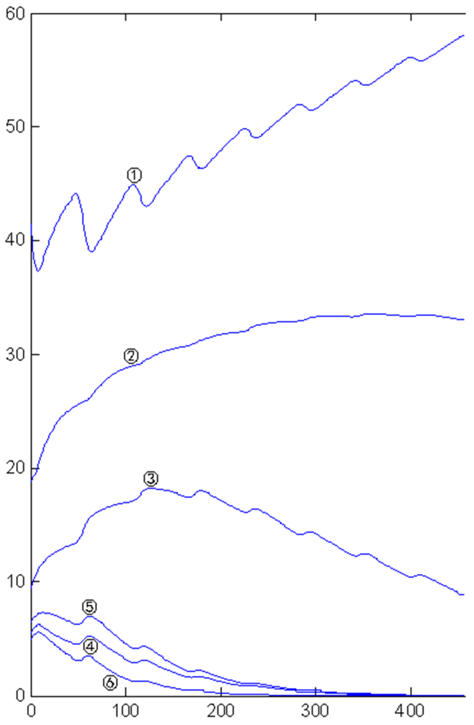
Moreover, to investigate the intrinsic dimension estimation, in the experiment, the intermediate result after each deforming step was analyzed by PCA and the relative ratios of the primary components were recorded. The variation in such ratios for the six most significant components is shown in Figure 15. The six curves in Figure 15 are labeled with the numbers of component order. Figure 15 indicates that the most significant and second-most significant components had increasing proportion rates. But the ratios of the other four components decreased obviously with the deformation going on. This clearly revealed the data set had two main latent variables, which were just in accord with the rotating angle and size factors. The fluctuation of the curves in Figure 15 was due to the dynamic periodic adjustment of α1 and α2 described in Section 3.
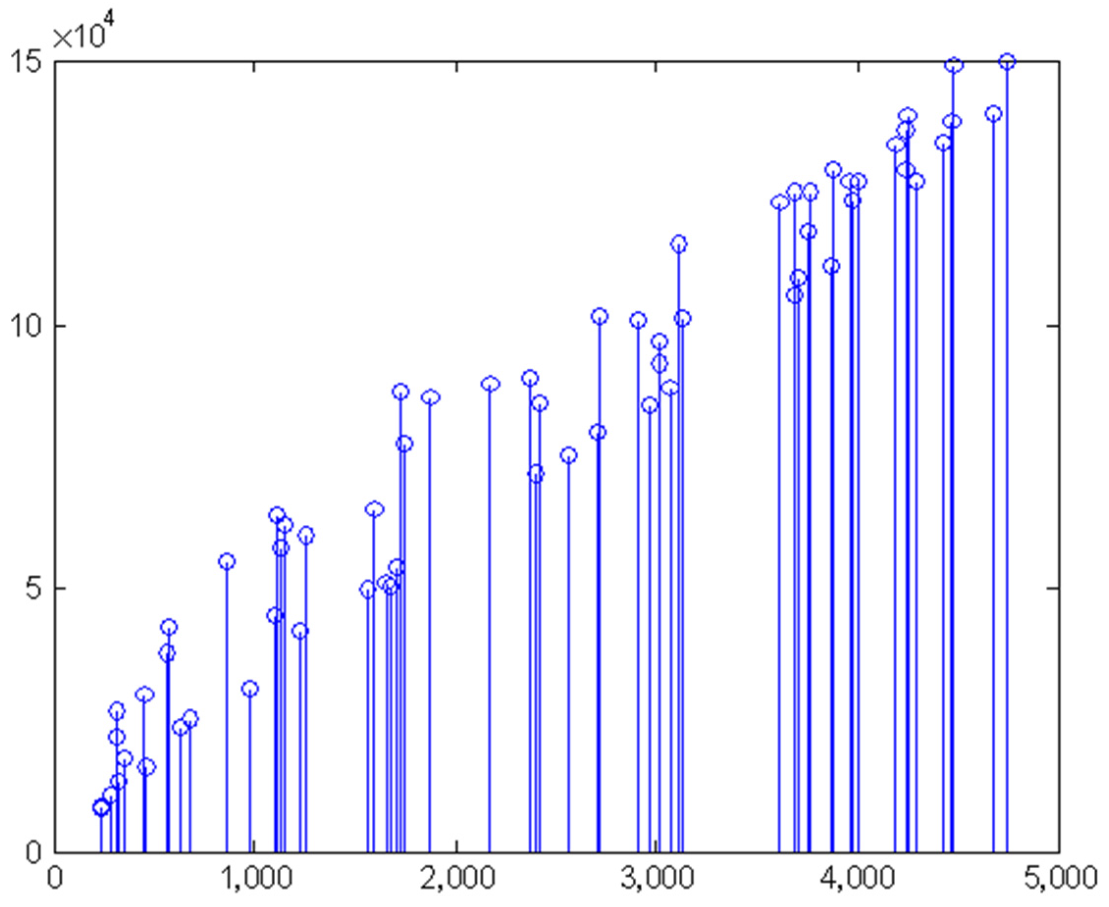
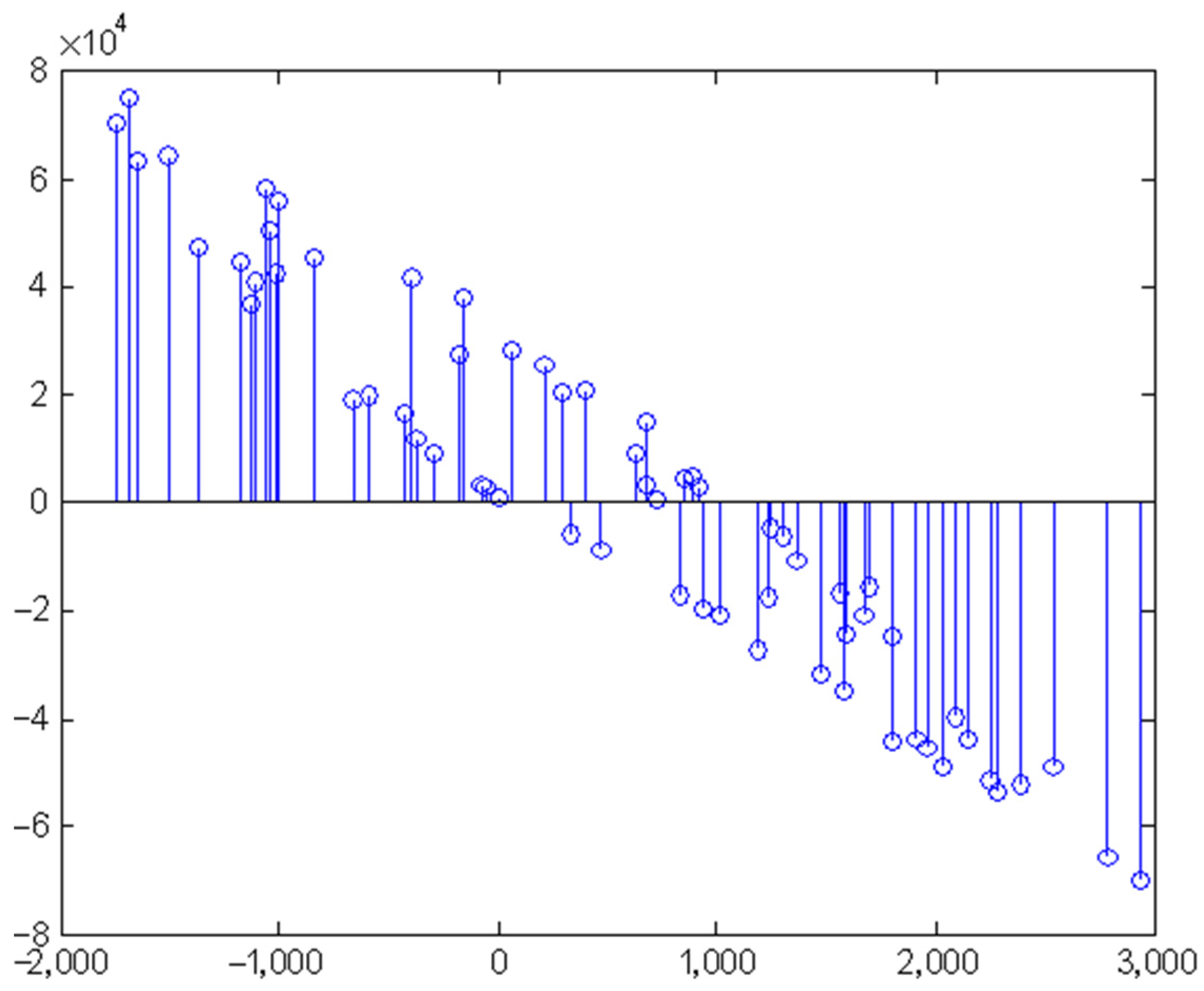
Experiments were performed on the “Extended Yale Face Database B”, which is groups of face images captured for different people [34]. The person and the camera keep motionless, but the illumination intensity and angle change. The image data set is from the Internet [35]. Figure 16 shows one group of images for a person. Figure 17 shows the final result of dimension reduction. The node points in Figure 17 represent the images, which are labeled with their corresponding numbers. The face images are also displayed near the corresponding nodes. The edges connect the neighbor points. In the result, the x-axis in Figure 17 can be interpreted as the illumination intensity factor and the y-axis represents the illumination angle. For quantitative analysis, the sum of pixel intensity was calculated for each image as the representation of illumination intensity. And the intensity difference between the left and right half of each image was also calculated as the representation of the illumination angle factor. Figure 18 shows the distribution of intensity summation along the x-axis in Figure 17, which indicates that the illumination intensity has an increasing tendency along the x-axis in Figure 17. Figure 19 shows the left–right difference in intensity for each image, which indicates that the illumination angle changes from right to left along the y-axis in Figure 17. Therefore, the DR result revealed the two factors underlying these face images.
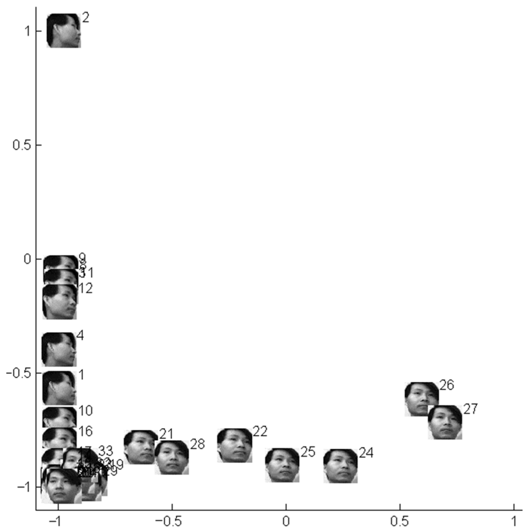
Experiments were performed for the cropped images of the “UMIST Face Database”, which includes image sequences captured when people turn their heads [36]. The image data set is from the Internet [37]. Figure 20 shows one group of images. Figure 21 shows the final DR result, where the nodes are labeled with numbers. The corresponding images are also displayed. The x-axis represents the major dimension, which reflects the angle between the head’s orientation and the posteroanterior direction. Interestingly, there existed a non-negligible second dimension in the result, which reflected the angle between the head’s orientation and the 45-degree direction of the face. In Figure 21, this dimension reaches its minimum at node point 17 (i.e., the 17th image in the sequence), which is the one closest to the visual angle of 45 degrees. On the other hand, long-term practice and experience in photography indicate that the most suitable angle of view to demonstrate the 3D effect of faces or objects is 45 degrees. The experiment indicated that the proposed model had the potential to reveal implicit features of the data sets.

3.3. Comparison with Typical Manifold Learning Methods

Manifold learning methods can be divided into two categories: global preserving embedding and local preserving embedding. Isomap and LLE are two representative methods of the two categories, respectively. In the experiments, the proposed method demonstrated its robustness on various data sets compared to Isomap and LLE.
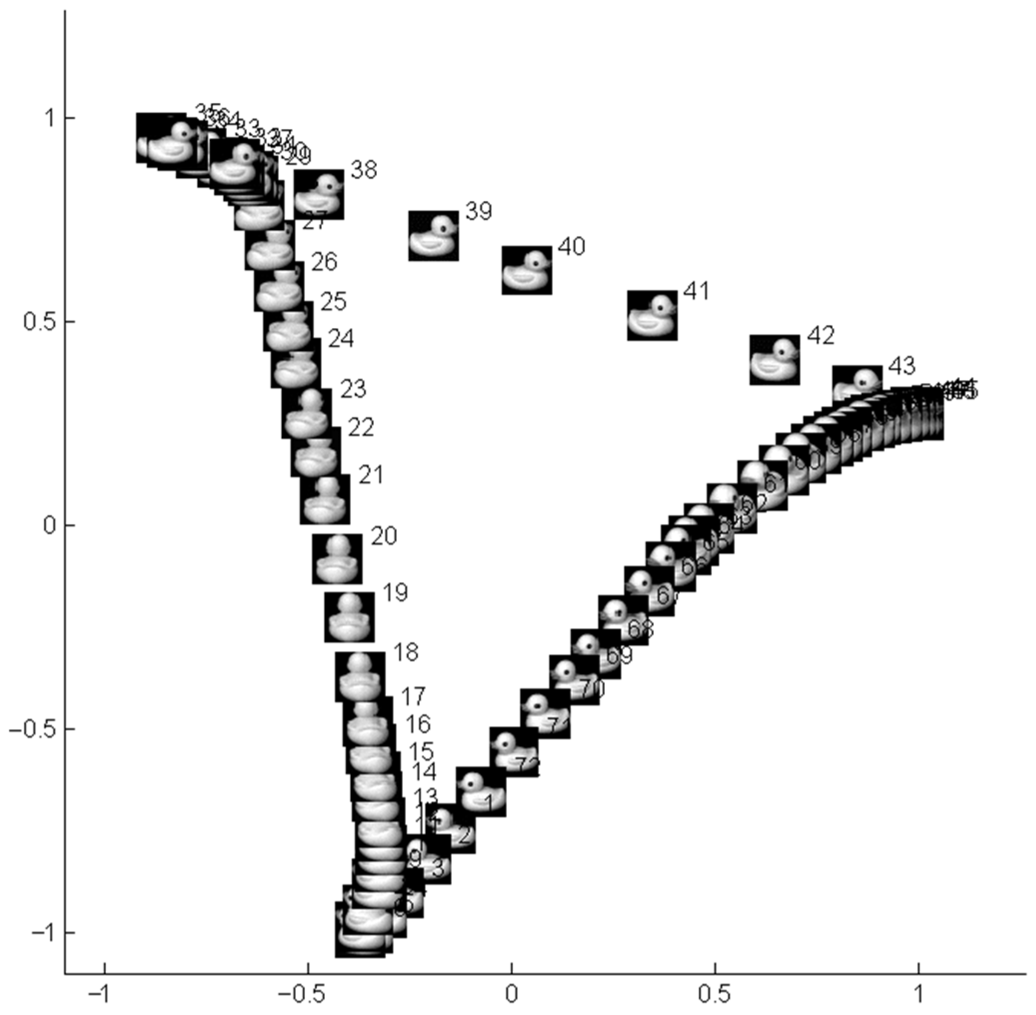
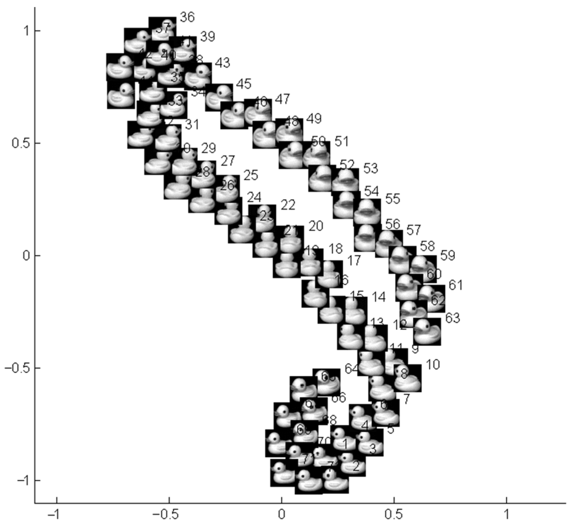
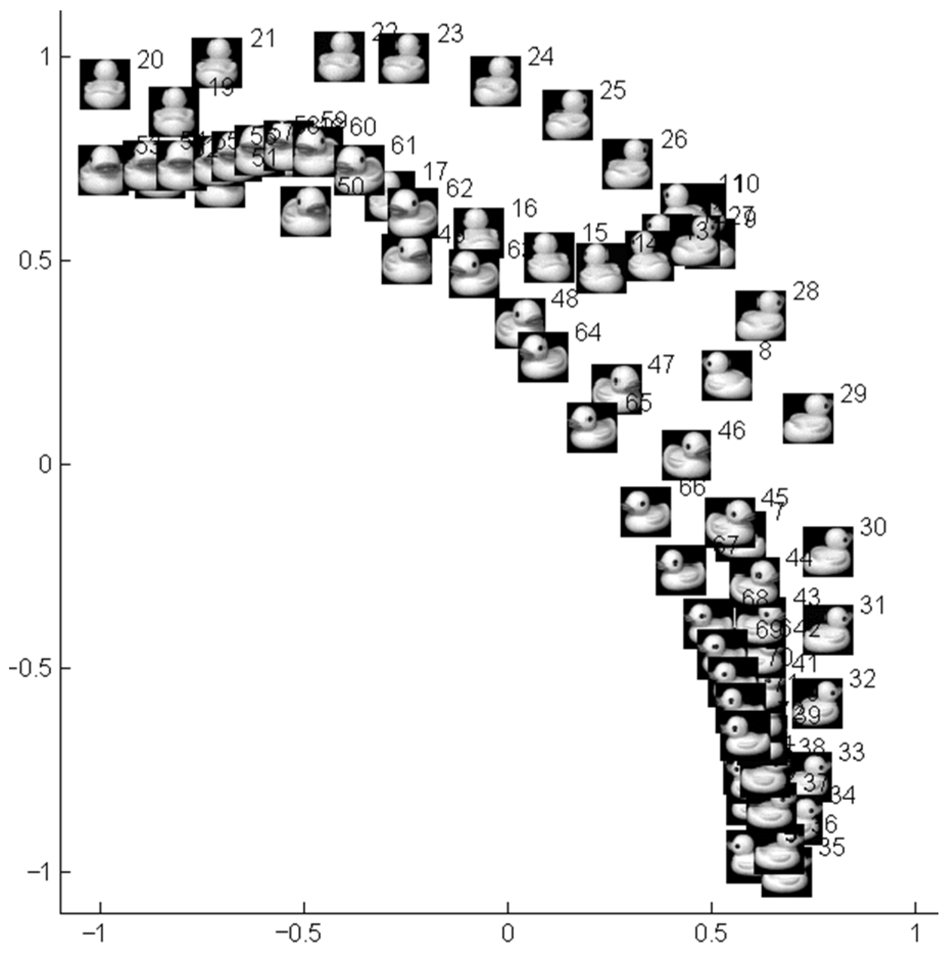
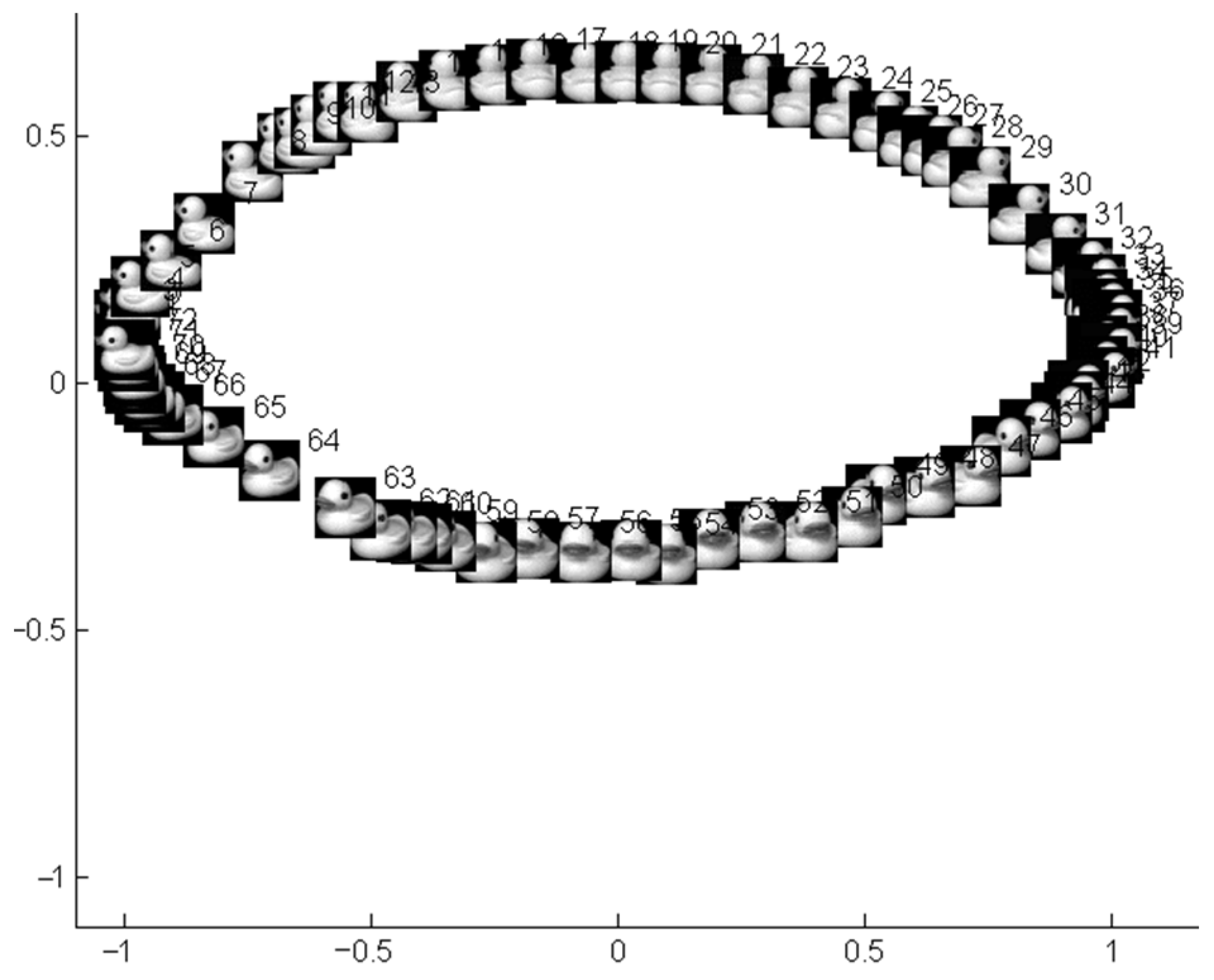
Figure 22 and Figure 23 show the 2D embedding results of the toy image sequence in Figure 10 by Isomap and LLE, respectively. The image sequence in Figure 10 has a smooth change in viewing angle and size, but the embedding result by LLE had several obviously sharp bends on the curve of embedded points, which deviated from the characteristics of the data itself. On the other hand, the DR results of the proposed method and the Isomap method accorded with the data characteristics well.
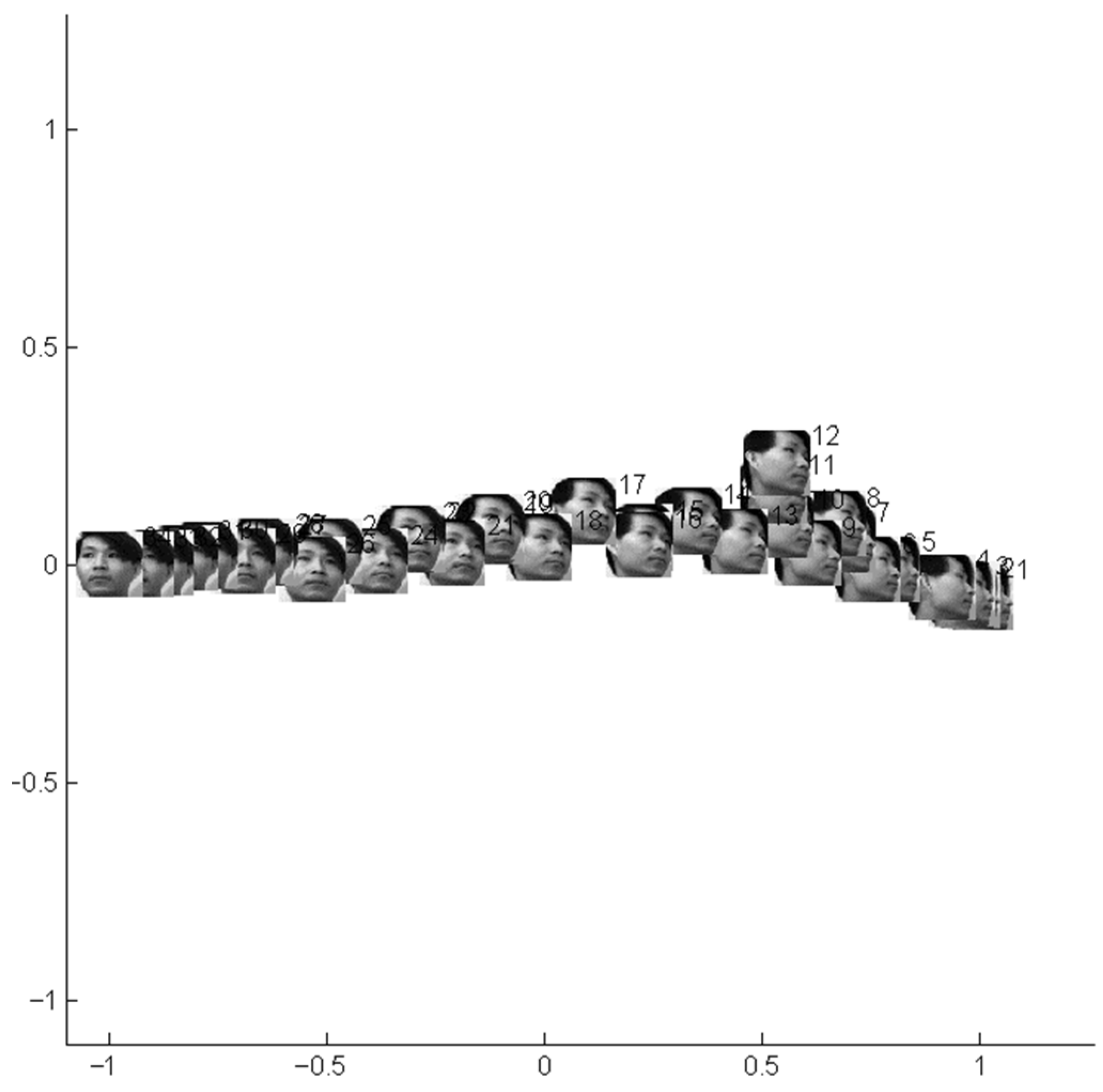
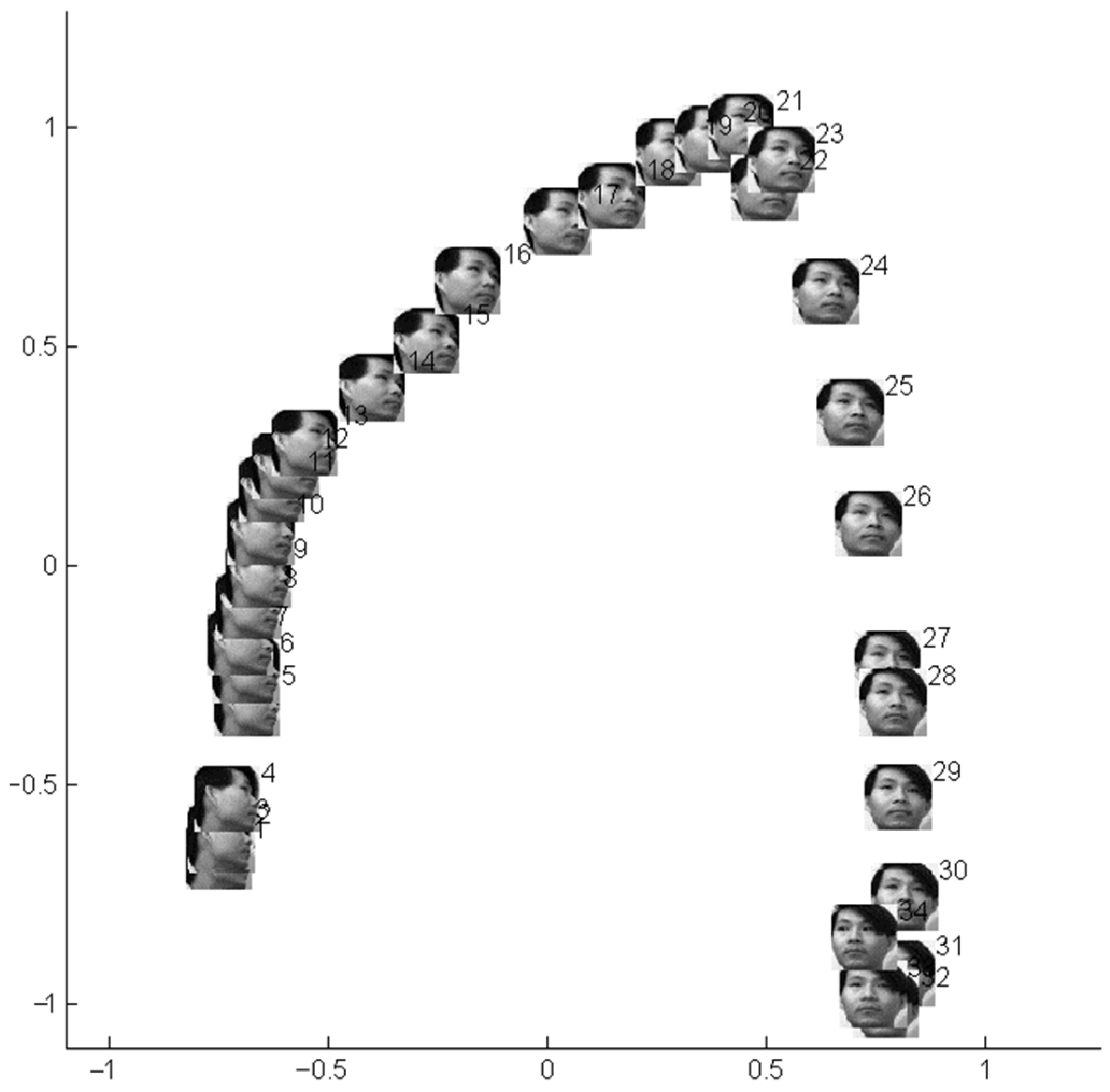
Figure 24 and Figure 25 show the 2D embedding results of the image sequence in Figure 20 by Isomap and LLE, respectively. It is obvious that, in the embedding result by Isomap, the embedded data points almost formed a line rather than a 2D curve. On the other hand, the DR results of the proposed method and the LLE method clearly indicated the 2D structure underlying the original image data.
In addition to the two kinds of typical manifold learning methods, the proposed model was also compared with improved or new types of learning approaches including t-distributed stochastic neighbor embedding (t-SNE), local tangent space alignment (LTSA), and locality preserving projection (LPP). Figure 26, Figure 27 and Figure 28 are the DR results for the toy image sequence in Figure 10 by t-SNE, LTSA, and LPP, respectively. In Figure 26 and Figure 27, although local parts of the results may reflect the local neighborhood structure of the data points, the whole 2D structure of the mapping result can not represent the original data topology structure. Figure 28 shows that the LPP method had a similar reasonable DR result.
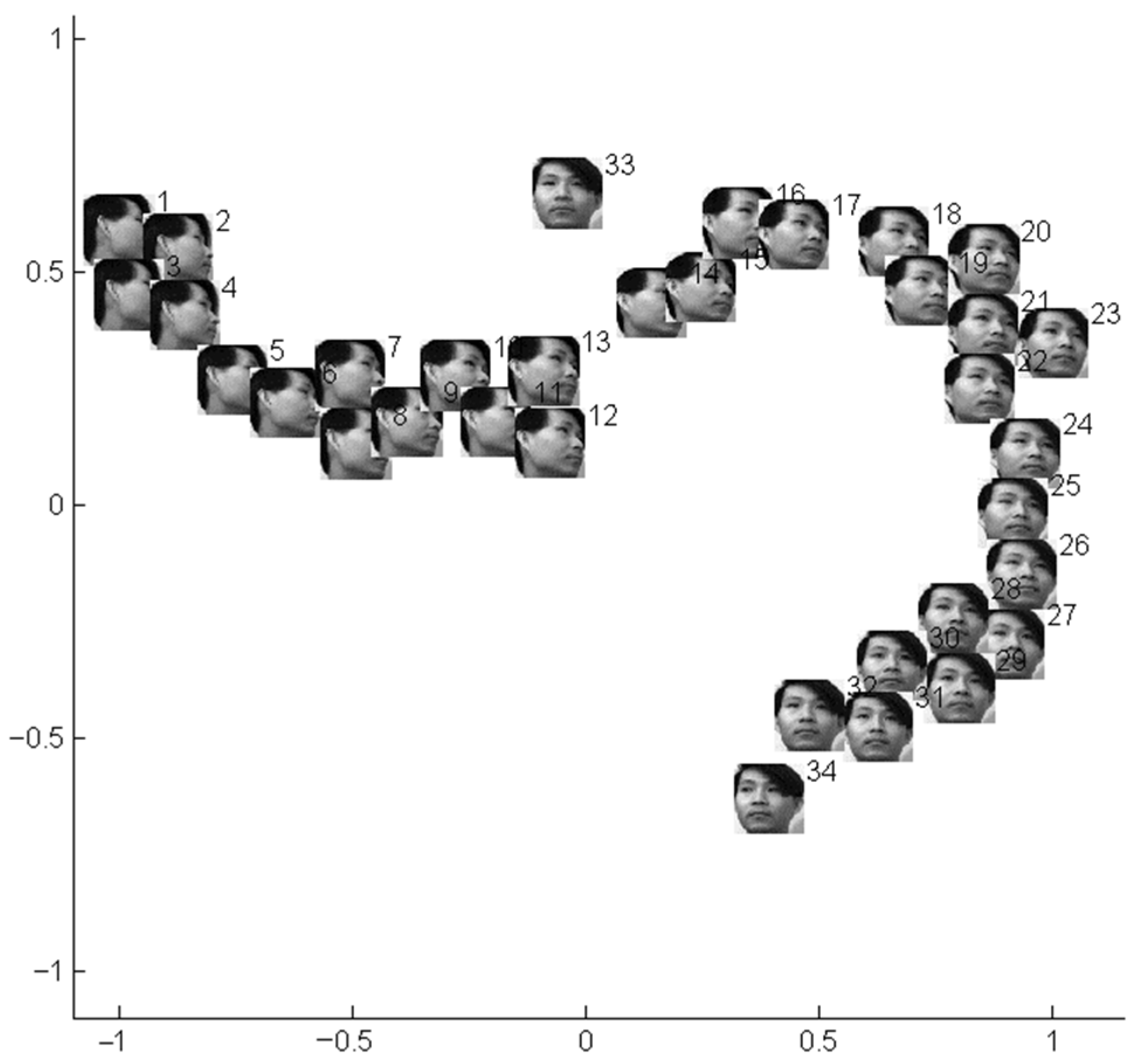
Figure 29, Figure 30 and Figure 31 are the DR results for the image sequence in Figure 20 by t-SNE, LTSA, and LPP, respectively. In Figure 29, the data point with No. 33 was obviously misplaced by the 2D mapping of t-SNE. In Figure 30, the local neighborhood structure and the global topology structure of the data points are not reflected in the 2D mapping result of LTSA. Figure 30 shows that the LPP method had a similar reasonable DR result compared to the proposed model, although the data points with No. 22 and No. 23 were misplaced in the DR result by LPP.
The comparison experiments clearly indicated the advantage of the robustness and self-adaption of the proposed model. The model’s robustness derives mainly from the soft neighborhood defined by Equations (1) and (2), which eliminate the interference of misjudging neighbor points. However, most manifold learning approaches greatly depend on the parameter of neighborhood size (i.e., the number of neighbor points), which may lead to unsatisfactory DR results due to the misjudgment of neighbor points. The model’s self-adaption derives mainly from the self-evolutionary mechanism of the deformation, which is guided by an intrinsic vector field defined completely by the current manifold shape. However, the mathematical frameworks in most manifold learning approaches are fixed, which may be suitable for only limited kinds of data sets.

4. Conclusions and Discussion

In this paper, to improve the robustness of manifold learning, a self-evolution model for dimension reduction is proposed based on the autonomous flattening deformation of data manifolds. Two different kinds of virtual interactions between data points are defined. The repulsion interaction is defined to make the manifold flattened, while the elastic interaction is defined to preserve the manifold’s topological structure in the flattening process. The deformation of data manifold is guided by the two interactions, and dimension reduction is achieved as an emergent result of the autonomous deformation. The proposed topological deformation learning provides a new self-organized model to understand and interpret dimension reduction and feature extraction in learning.
With analogy to the attractor in differential dynamic systems, the flattening effect of the proposed deforming vector field can be interpreted as the evolution of the data manifold to an “attracting state”. If all the data points are in the same low-dimensional hyperplane in Rn, the attracting or repulsive vectors between any two of them are all in the same hyperplane. Moreover, the displacement vectors of the data points under such attracting and repulsive interactions are also within the same hyperplane, and no point will move out of this low-dimensional hyperplane. Thus, it can be regarded as an “attracting state”. The evolution of the data manifold under the proposed deforming field will approach such an attractive state (i.e., the manifold will be flattened).
To overcome the problem caused by non-uniform sampling (or “short-circuit edge”) and neighbor point misjudging, which are common in practical learning tasks, the soft neighborhood is proposed as an adaptive way to determine the interactions between neighbor points. This improvement guarantees a sufficient number of neighboring points, meanwhile eliminating the interference of fake neighboring points, which may make the learning result meaningless. It guarantees the robustness of the proposed model, which outperformed other typical methods in the comparison experiments.
The experiments on test data manifolds such as S-surface and Gaussian surfaces prove that the proposed method can effectively flatten the two typical surfaces of the bending or concave–convex case. Other experiments were carried out on real-world data sets, including object images with changing size and angle of view, face images with changing illumination angle and intensity, and also face image sequences captured when the subjects turn their heads. The experimental results prove that effective dimension reduction can be achieved by the proposed method. The intrinsic dimensions can be revealed, and each dimension has a meaningful interpretation. It also has the potential to reveal implicit features in the data set. Moreover, compared to the typical and new types of manifold learning methods, the proposed method provides more robust results. Further study will investigate detailed characteristics of the final stable shape of the deforming manifold and its relationship between the algorithm parameters (i.e., weight coefficients), which may provide inspirations for a new design of method in dimension reduction.

Author Contributions

Conceptualization, X.Z.; methodology, X.Z. and N.M.; software, X.Z.; validation, X.Z. and N.M.; formal analysis, N.M.; resources, N.M.; data curation, N.M.; writing—original draft preparation, X.Z.; writing—review and editing, X.Z. and N.M.; visualization, N.M.; supervision, N.M.; project administration, X.Z. All authors have read and agreed to the published version of the manuscript.

Funding

This research received no external funding.

Data Availability Statement

Not applicable.

Conflicts of Interest

The authors declare no conflict of interest.

References

  1. Jia, W.; Sun, M.; Lian, J.; Hou, S. Feature dimensionality reduction: A review. Complex Intell. Syst. 2022, 8, 2663–2693. [Google Scholar] [CrossRef]
  2. Ghosh, D. Sufficient Dimension Reduction: An Information-Theoretic Viewpoint. Entropy 2022, 24, 167. [Google Scholar] [CrossRef] [PubMed]
  3. Riznyk, V. Big Data Process Engineering under Manifold Coordinate Systems. WSEAS Trans. Inf. Sci. Appl. 2021, 18, 7–11. [Google Scholar] [CrossRef]
  4. Donoho, D.L. High-Dimensional Data Analysis: The Curses and Blessing of Dimensionality. In Proceedings of the of AMS Mathematical Challenges of the 21st Century, Los Angeles, LA, USA, 7–12 August 2000; pp. 1–32. [Google Scholar]
  5. Ray, P.; Reddy, S.S.; Banerjee, T. Various dimension reduction techniques for high dimensional data analysis: A review. Artif. Intell. Rev. 2021, 54, 3473–3515. [Google Scholar] [CrossRef]
  6. Ayesha, S.; Hanif, M.K.; Talib, R. Overview and comparative study of dimensionality reduction techniques for high dimensional data. Inf. Fusion 2020, 59, 44–58. [Google Scholar] [CrossRef]
  7. Langdon, C.; Genkin, M.; Engel, T.A. A unifying perspective on neural manifolds and circuits for cognition. Nat. Rev. Neurosci. 2023, 24, 363–377. [Google Scholar] [CrossRef] [PubMed]
  8. Cohen, U.; Chung, S.Y.; Lee, D.D.; Sompolinsky, H. Separability and geometry of object manifolds in deep neural networks. Nat. Commun. 2020, 11, 746. [Google Scholar] [CrossRef] [PubMed]
  9. Seung, H.S.; Lee, D.D. The manifold ways of perception. Science 2000, 290, 2268–2269. [Google Scholar] [CrossRef]
  10. Tenenbaum, J.B.; Silva, V.; Langford, J.C. A Global Geometric Framework for Nonlinear Dimensionality Reduction. Science 2000, 290, 2319–2323. [Google Scholar] [CrossRef]
  11. Roweis, S.T.; Saul, L.K. Nonlinear Dimensionality Reduction by Locally Linear Embedding. Science 2000, 290, 2323–2326. [Google Scholar] [CrossRef]
  12. Belkin, M.; Niyogi, P. Laplacian Eigenmaps for dimensionality reduction and data representation. Neural Comput. 2003, 15, 1373–1396. [Google Scholar] [CrossRef]
  13. Weinberger, K.Q.; Saul, L.K. Unsupervised learning of image manifolds by semidefinite programming. Int. J. Comput. Vision 2006, 70, 77–90. [Google Scholar] [CrossRef]
  14. Lin, T.; Zha, H.B. Riemannian Manifold Learning. IEEE Trans. Pattern Anal. Mach. Intell. 2008, 30, 796–809. [Google Scholar] [PubMed]
  15. Ran, R.; Qin, H.; Zhang, S.; Fang, B. Simple and Robust Locality Preserving Projections Based on Maximum Difference Criterion. Neural Process Lett. 2022, 54, 1783–1804. [Google Scholar] [CrossRef]
  16. Maaten, L.; Hinton, G. Visualizing Data using t-SNE. J. Mach. Learn. Res. 2008, 9, 2579–2605. [Google Scholar]
  17. Zhang, Z.Y.; Zha, H.Y. Principal Manifolds and Nonlinear Dimensionality Reduction via Tangent Space Alignment. SIAM J. Sci. Comput. 2004, 26, 313–338. [Google Scholar] [CrossRef]
  18. Yan, S.C.; Xu, D.; Zhang, B.Y.; Zhang, H.J.; Yang, Q.; Lin, S. Graph embedding and extensions: A general framework for dimensionality reduction. IEEE Trans. Pattern Anal. Mach. Intell. 2007, 29, 40–51. [Google Scholar] [CrossRef] [PubMed]
  19. Zhang, T.; Tao, D.; Li, X.; Yang, J. Patch Alignment for Dimensionality Reduction. IEEE Trans. Knowl. Data Eng. 2009, 21, 1299–1313. [Google Scholar] [CrossRef]
  20. Huang, X.; Wu, L.; Ye, Y. A Review on Dimensionality Reduction Techniques. Int. J. Pattern Recogni. Artif. Intell. 2019, 33, 1950017. [Google Scholar] [CrossRef]
  21. Bengio, Y.; Larochelle, H.; Vincent, P. Non-local manifold parzen windows. In Proceedings of the Advances in Neural Information Processing Systems, Vancouver, BC, Canada, 5–8 December 2005; pp. 115–122. [Google Scholar]
  22. Bengio, Y.; Monperrus, M.; Larochelle, H. Nonlocal estimation of manifold structure. Neural Comput. 2006, 18, 2509–2528. [Google Scholar] [CrossRef]
  23. Bengio, Y.; Monperrus, M. Non-local manifold tangent learning. In Proceedings of the Advances in Neural Information Processing Systems, Vancouver, BC, Canada, 13–18 December 2004; pp. 129–136. [Google Scholar]
  24. Xu, X.Z.; Liang, T.M.; Zhu, J.; Zheng, D.; Sun, T.F. Review of classical dimensionality reduction and sample selection methods for large-scale data processing. Neurocomputing 2019, 328, 5–15. [Google Scholar] [CrossRef]
  25. Zeng, X.H. Applications of average geodesic distance in manifold learning. In Proceedings of the 3rd International Conference on Rough Sets and Knowledge Technology, Chengdu, China, 17–19 May 2008; pp. 540–547. [Google Scholar]
  26. Hassanien, A.E.; Emary, E. Swarm Intelligence: Principles, Advances, and Applications; CRC Press: Boca Raton, FL, USA, 2018. [Google Scholar]
  27. Slowik, A. Swarm Intelligence Algorithms; CRC Press: Boca Raton, FL, USA, 2021. [Google Scholar]
  28. Iba, H. AI and SWARM: Evolutionary Approach to Emergent Intelligence; CRC Press: Boca Raton, FL, USA, 2019. [Google Scholar]
  29. Nguyen, H.T.; Walker, C.L.; Walker, E.A. A First Course in Fuzzy Logic; Chapman and Hall/CRC: Boca Raton, FL, USA, 2018. [Google Scholar]
  30. Viksten, F.; Forssen, P.-E.; Johansson, B.; Moe, A. Comparison of Local Image Descriptors for Full 6 Degree-of-Freedom Pose Estimation. In Proceedings of the IEEE International Conference on Robotics and Automation, Kobe, Japan, 12–17 May 2009; pp. 2779–2786. [Google Scholar]
  31. Object Pose Estimation Database. Available online: https://www.cvl.isy.liu.se/research/objrec/posedb/index.html (accessed on 9 February 2023).
  32. Nene, S.A.; Nayar, S.K.; Murase, H. Columbia Object Image Library (COIL-20); Technical Report CUCS-005-96; Columbia University: New York, NY, USA, 1996. [Google Scholar]
  33. Columbia University Image Library. Available online: https://www.cs.columbia.edu/CAVE/software/softlib/coil-20.php (accessed on 26 May 2022).
  34. Georghiades, A.S.; Belhumeur, P.N.; Kriegman, D.J. From Few to Many: Illumination Cone Models for Face Recognition under Variable Lighting and Pose. IEEE Trans. Pattern Anal. Mach. Intell. 2001, 23, 643–660. [Google Scholar] [CrossRef]
  35. Extended Yale Face Database B. Available online: http://vision.ucsd.edu/~leekc/ExtYaleDatabase/ExtYaleB.html (accessed on 26 May 2022).
  36. Graham, D.B.; Allinson, N.M. Characterizing Virtual Eigensignatures for General Purpose Face Recognition. In Face Recognition: From Theory to Applications; NATO ASI Series F, Computer and Systems Sciences; Wechsler, H., Phillips, P.J., Bruce, V., Soulié, F.F., Huang, T.S., Eds.; Fogelman-Soulie; Springer: Berlin/Heidelberg, Germany, 1998; Volume 163, pp. 446–456. [Google Scholar]
  37. Sam Roweis: Data for MATLAB. Available online: https://cs.nyu.edu/~roweis/data.html (accessed on 29 June 2022).
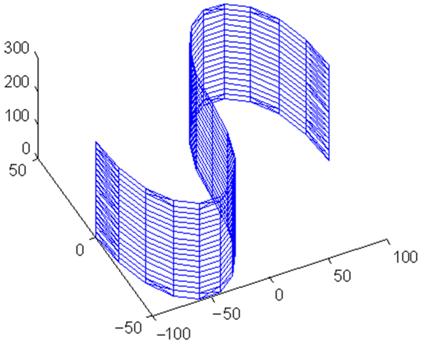
Figure 1. The mesh of the S-surface where neighboring points are connected by edges.
Symmetry 15 01995 g001
Figure 2. The demonstration of the displacement vectors on the initial data mesh in Figure 1.
Symmetry 15 01995 g002
Figure 3. The shapes of the manifold after some deforming steps in the simulation of the proposed method. (a) 20 steps, (b) 70 steps, (c) 100 steps, (d) 190 steps, (e) 220 steps, (f) 320 steps.
Symmetry 15 01995 g003
Figure 4. The Gaussian surface (with the variance value 6.0) and the deforming result in R3. (a) The Gaussian surface, (b) the deforming result in R3.
Symmetry 15 01995 g004
Figure 5. The dimension reduction result of Figure 4a in R2.
Symmetry 15 01995 g005
Figure 6. The Gaussian surface (with variance value 2) and the deforming result in R3. (a) The Gaussian surface, (b) the deforming result in R3.
Symmetry 15 01995 g006
Figure 7. The dimension reduction result of Figure 6a in R2.
Symmetry 15 01995 g007
Figure 8. The auto fuse image set.
Symmetry 15 01995 g008
Figure 9. The dimension reduction result of the auto fuse image set in R2.
Symmetry 15 01995 g009
Figure 10. The toy image sequence in the “Columbia Object Image Library (COIL-20)”.
Symmetry 15 01995 g010
Figure 11. The dimension reduction result of the toy image sequence in R2.
Symmetry 15 01995 g011
Figure 12. The detailed demonstration of area (A) in Figure 11.
Symmetry 15 01995 g012
Figure 13. The detailed demonstration of area (B) in Figure 11.
Symmetry 15 01995 g013
Figure 14. The detailed demonstration of area (C) in Figure 11.
Symmetry 15 01995 g014
Figure 15. The relative ratios of the first six primary components in the deforming process.
Symmetry 15 01995 g015
Figure 16. One group of face images for a person in the “Extended Yale Face Database B”.
Symmetry 15 01995 g016
Figure 17. The dimension reduction result for the image sequence in Figure 16.
Symmetry 15 01995 g017
Figure 18. The intensity summation for each image along the x-axis in Figure 17.
Symmetry 15 01995 g018
Figure 19. The left–right difference of intensity for each image along the y-axis in Figure 17.
Symmetry 15 01995 g019
Figure 20. One group of the images from the cropped images of the “UMIST Face Database”.
Symmetry 15 01995 g020
Figure 21. The dimension reduction result for the image sequence in Figure 20.
Symmetry 15 01995 g021
Figure 22. The two-dimensional mapping of the toy image set by Isomap.
Symmetry 15 01995 g022
Figure 23. The two-dimensional mapping of the toy image set by LLE.
Symmetry 15 01995 g023
Figure 24. The two-dimensional mapping of the face image set by Isomap.
Symmetry 15 01995 g024
Figure 25. The two-dimensional mapping of the face image set by LLE.
Symmetry 15 01995 g025
Figure 26. The two-dimensional mapping of the toy image set by t-SNE.
Symmetry 15 01995 g026
Figure 27. The two-dimensional mapping of the toy image set by LTSA.
Symmetry 15 01995 g027
Figure 28. The two-dimensional mapping of the toy image set by LPP.
Symmetry 15 01995 g028
Figure 29. The two-dimensional mapping of the face image set by t-SNE.
Symmetry 15 01995 g029
Figure 30. The two-dimensional mapping of the face image set by LTSA.
Symmetry 15 01995 g030
Figure 31. The two-dimensional mapping of the face image set by LPP.
Symmetry 15 01995 g031
Disclaimer/Publisher’s Note: The statements, opinions and data contained in all publications are solely those of the individual author(s) and contributor(s) and not of MDPI and/or the editor(s). MDPI and/or the editor(s) disclaim responsibility for any injury to people or property resulting from any ideas, methods, instructions or products referred to in the content.