Novel Computations of the Time-Fractional Coupled Korteweg–de Vries Equations via Non-Singular Kernel Operators in Terms of the Natural Transform

Abstract

In the present research, we establish an effective method for determining the time-fractional coupled Korteweg–de Vries (KdV) equation’s approximate solution employing the fractional derivatives of Caputo–Fabrizio and Atangana–Baleanu. KdV models are crucial because they can accurately represent a variety of physical problems, including thin-film flows and waves on shallow water surfaces. Some theoretical physical features of quantum mechanics are also explained by the KdV model. Many investigations have been conducted on this precisely solvable model. Numerous academics have proposed new applications for the generation of acoustic waves in plasma from ions and crystal lattices. Adomian decomposition and natural transform decomposition techniques are combined in the natural decomposition method (NDM). We first apply the natural transform to examine the fractional order and obtain a recurrence relation. Second, we use the Adomian decomposition approach to the recurrence relation, and then, using successive iterations and the initial conditions, we can establish the series solution. We note that the proposed fractional model is highly accurate and valid when using this technique. The numerical outcomes demonstrate that only a small number of terms are required to arrive at an approximation that is exact, efficient, and trustworthy. Two examples are given to illustrate how the technique performs. Tables and 3D graphs display the best current numerical and analytical results. The suggested method provides a series form solution, which makes it quite easy to understand the behavior of the fractional models.

1. Introduction

Fractional calculus (FC) is a 17th-century invention that generalizes integer-order calculus to arbitrary-order calculus. The primary advantage of FC is that it describes a beneficial technique for researching memory and genetic characteristics in a wide range of phenomena. Furthermore, ordinary calculus is a subset of FC. The fundamental research of fractional derivatives has advanced rapidly in recent decades. Fractional calculus has received much attention in the last thirty years or more. Several academics have noticed that developing unique fractional derivatives (FDs) with distinct singular or nonsingular kernels is critical to address the demand for modeling real-world problems in various areas. Because most FDs do not have perfect solutions, approximations and numerical techniques must be used. More information on the definitions and properties of fractional derivatives can be checked at [1]. Over the last five decades, research on the theory and application of differential equations (DEs) in terms of Caputo FD has been achieved [2,3]. However, the Caputo FD has a unique kernel. Caputo and Fabrizio offered a solution to the solitary kernel problem using an exponential function in the last decade [4]. Although this operator is local, it has several concerns. The corresponding integral is not fractional in the fractional order derivative. Atangana and Baleanu work hard to overcome local issues [5]. They designed the Liouville–Caputo and Riemann–Liouville derivatives of the modified Mittag–Leffler function. Actually, this derivative is not only a differential operator; it may also be thought of as a filter regulator. This interesting derivative also has the benefit of explaining some of the macroscopic behavior of certain materials. Numerous researchers have been closely observing these derivatives’ stimulating behaviors in recent years [6,7,8].

Non-singular FDs have been employed in several models. Several models have recently been studied for non-singular FDs [9,10]. The authors investigated the dynamics of several physical issues using the Atangana–Baleanu (AB) and Caputo–Fabrizio (CF) FDs. Wang et al. used non-singular FD to develop a model for bank data with real field data from 2004 to 2014 [11]. They illustrate the fractional ABC operator’s better accuracy and adaptability and how it may be used with comfort to simulate such real-world events. Saifullah et al. used the non-singular FD in the CF sense to show the complicated progression of HIV infection [12]. Khan et al. used non-singular FDs to investigate the nonlinear Schrodinger equation’s wave propagation [13]. Rahman et al. examined the ${\Phi }^4-$equation with nonsingular FDs [14]. Khan et al. examined the KdV–Burger equation’s wave dynamics assuming non-singular FDs [15]. The works listed in the citations [16,17,18] are all helpful. The fractional calculus has many uses; see [19,20,21,22,23,24] for a few examples.

FC has been used to model physical and engineering processes best represented by differential fractional equations (FDEs). In recent decades, FDEs have been extensively used in numerous engineering and applied science fields. Nonlinear differential equations define most of the phenomena in nature. Thus, researchers pay more attention to the different branches of science and engineering to try to solve them. However, finding an exact solution is hard due to the involvement of nonlinear parts in these equations. The solutions of nonlinear FPDEs are of great concern in mathematics and useful applications [25,26,27]. Consequently, knowing how to build a reliable technique to obtain the approximate or the exact solution of FPDEs is of great interest in the field of research of fractional models. Numerous analytical techniques have been used to find the solution of these problems. Such as iterative Laplace transform method [28], Laplace variational iteration method [29], approximate-analytical method [30], Laplace Adomian decomposition method [31], optimal homotopy asymptotic method [32], reduced differential transform method [33], homotopy analysis method [34], Natural transform decomposition method [35], Adomian decomposition method [36] and many more [37,38,39,40,41].

The Korteweg–de Vries (KdV) equation is a sort of partial differential equation that has recently been employed in defining several physical occurrences as an example of the formation and association of nonlinear waves. It was constructed as a modified equation controlling the movement of one-dimensional, large, small-amplitude surface gravity waves in a shallow water channel, as demonstrated in [42]. The KdV equation is currently being investigated in various physical science fields, such as stratified internal waves, plasma physics, ion-acoustic waves, lattice dynamics, and collision-free hydromagnetic waves [43]. A KdV model has been employed in quantum physics to explain several hypothetical physical phenomena. It is applied in fluid dynamics, aerodynamics, and continuum mechanics as a model for shock wave production, turbulence, solitons, mass transport, and boundary layer behavior [44]. In this study, we derive an analytical solution to the nonlinear coupled time-fractional KdV equations that are provided by:

$$\begin{array}{cc}\hfill & D_{\zeta }^{\beta }\mathbf{F}(\omega ,\zeta )=\mathbf{a}{\mathbf{F}}_{\omega \omega \omega }(\omega ,\zeta )+\mathbf{b}\mathbf{F}(\omega ,\zeta ){\mathbf{F}}_{\omega }(\omega ,\zeta )+\mathbf{c}\mathbf{G}(\omega ,\zeta ){\mathbf{G}}_{\omega }(\omega ,\zeta ),\hfill \\ \hfill & D_{\zeta }^{\beta }\mathbf{G}(\omega ,\zeta )=\mathbf{d}{\mathbf{F}}_{\omega \omega \omega }(\omega ,\zeta )-\mathbf{e}\mathbf{G}(\omega ,\zeta ){\mathbf{G}}_{\omega }(\omega ,\zeta ),0<\beta \le 1,\hfill \end{array}$$

(1)

subjected to initial sources

$$\mathbf{J}(\omega ,0)=h_1\left(\omega \right),\mathbf{K}(\omega ,0)=h_2\left(\omega \right).$$

(2)

where $\mathbf{a},\mathbf{d}<0$; $\mathbf{b},\mathbf{c}$ and $\mathbf{e}$ stand for constant parameters. Numerous academics have explored the KdV equation, which has applications in analyzing shallow-water waves and many other physical phenomena.

The Adomian decomposition method, which yields accurate solutions in the form of a convergent series, is a well-known technique for solving homogeneous and nonhomogeneous, linear and nonlinear, homogeneous and nonlinear differential and partial differential equations, as well as integro differential and fractional differential equations. Without the need for linearization or disturbance, the Adomian decomposition method has been successfully and efficaciously applied to examine issues that have arisen in science and technology. On the other hand, the Adomian decomposition method requires a significant quantity of computer memory and more time for computational work. Therefore, it is inevitable that this method will be used with already-existing transform methods. Differential equations were solved by combining a number of transforms with additional methods. In [45,46], the natural decomposition method (NDM), a linked natural transform and Adomian decomposition approach, was developed for solving differential equations. It provides an approximation solution in series form. The central theme of this work is to solve time-fractional coupled KdV equations NTDM. Numerous studies have employed the NTDM to obtain approximate analytical solutions; it generated accurate and closely convergent outcomes.

This work is structured as follows. Section 2 defines and describes the natural transform’s properties. Section 3 describes the overall implementation of the proposed technique. Section 4 covers the new technique and compares it to two different ways using two examples and presents tables and graphs to validate the NTDM. Section 5 contains the manuscript’s conclusion.

2. Important Notations

Definition 1. 

The non-integer Riemann–Liouville (RL) integral operator is defined [47]

$$\begin{array}{cc}\hfill I^{\beta }j\left(\eta \right)=& \frac{1}{\Gamma \left(\beta \right)}{\int }_0^{\eta }{(\eta -\wp )}^{\beta -1}j(\wp )d\wp ,\beta >0,\eta >0,\hfill \\ \hfill and{I}^{0}j\left(\eta \right)=& j\left(\eta \right).\hfill \end{array}$$

(3)

Definition 2. 

The non-integer derivative in Caputo sense is defined as [47]

$$\begin{array}{c}\hfill D_{\eta }^{\beta }j\left(\eta \right)=I^{\gamma -\beta }{D}^{\gamma }j\left(\eta \right)=\frac{1}{\gamma -\beta }{\int }_0^{\eta }{(\eta -\wp )}^{\gamma -\beta -1}{j}^{\left(\gamma \right)}(\wp )d\wp ,\end{array}$$

(4)

for $\gamma -1<\beta \le \gamma ,\gamma \in N,\eta >0,j\in C_{\wp }^{\gamma },\wp \ge -1$.

Definition 3. 

The non-integer derivative in CF sense is stated as [47]

$$\begin{array}{c}\hfill D_{\eta }^{\beta }j\left(\eta \right)=\frac{\mathcal{Z}\left(\beta \right)}{1-\beta }{\int }_0^{\eta }exp\left(\frac{-\beta (\eta -\wp )}{1-\beta }\right)D\left(j(\wp )\right)d\wp ,\end{array}$$

(5)

 having $0<\beta <1$ and $\mathcal{Z}\left(\beta \right)$ is a normalization function having $\mathcal{Z}\left(0\right)=\mathcal{Z}\left(1\right)=1$.

Definition 4. 

The non-integer derivative in the ABC sense is stated as [47]

$$\begin{array}{c}\hfill D_{\eta }^{\beta }j\left(\eta \right)=\frac{\mathcal{Z}\left(\beta \right)}{1-\beta }{\int }_0^{\eta }{E}_{\beta }\left(\frac{-\beta (\eta -\wp )}{1-\beta }\right)D\left(j(\wp )\right)d\wp ,\end{array}$$

(6)

 here $E_{\beta }\left(z\right)={\sum }_{m=0}^{\infty }\frac{z^m}{\Gamma (m\beta +1)}$.

Definition 5. 

The natural transform (NT) of $\mathbf{F}\left(\zeta \right)$ is as 

$$\begin{array}{c}\hfill \mathbb{N}\left(\mathbf{F}\left(\zeta \right)\right)=\mathcal{U}(\varsigma ,\kappa )={\int }_{-\infty }^{\infty }{e}^{-\varsigma \zeta }\mathbf{F}\left(\kappa \zeta \right)d\zeta ,\varsigma ,\kappa \in (-\infty ,\infty ),\end{array}$$

(7)

 and for $\zeta \in (0,\infty )$, the NT of $\mathbf{F}\left(\zeta \right)$ is as

$$\begin{array}{c}\hfill \mathbb{N}\left(\mathbf{F}\left(\zeta \right)H\left(\zeta \right)\right)={\mathbb{N}}^{+}={\mathcal{U}}^{+}(\varsigma ,\kappa )={\int }_0^{\infty }{e}^{-\varsigma \zeta }\mathbf{F}\left(\kappa \zeta \right)d\zeta ,\varsigma ,\kappa \in (0,\infty ).\end{array}$$

(8)

where $H\left(\zeta \right)$ is the Heaviside function.

Definition 6. 

The inverse NT of $\mathbf{F}(\varsigma ,\kappa )$ is as

$$\begin{array}{c}\hfill {\mathbb{N}}^{-1}\left[\mathcal{U}(\varsigma ,\kappa )\right]=\mathbf{F}\left(\zeta \right),\forall \zeta \ge 0.\end{array}$$

(9)

Lemma 1. 

Assume the NT of ${\mathbf{F}}_1\left(\zeta \right)$ and ${\mathbf{F}}_2\left(\zeta \right)$ are ${\mathcal{U}}_1(\varsigma ,\kappa )$ and ${\mathcal{U}}_2(\varsigma ,\kappa )$, so [48]

$$\begin{array}{c}\hfill \mathbb{N}[c_1{\mathbf{F}}_1\left(\zeta \right)+c_2{\mathbf{F}}_2\left(\zeta \right)]=c_1\mathbb{N}\left[{\mathbf{F}}_1\left(\zeta \right)\right]+c_2\mathbb{N}\left[{\mathbf{F}}_2\left(\zeta \right)\right]=c_1{\mathcal{U}}_1(\varsigma ,\kappa )+c_2{\mathcal{U}}_2(\varsigma ,\kappa ),\end{array}$$

(10)

having $c_1$ and $c_2$ constants.

Lemma 2. 

Assume the inverse NT of ${\mathbf{F}}_1\left(\zeta \right)$ and ${\mathbf{F}}_2\left(\zeta \right)$ ${\mathbf{F}}_1(\varsigma ,\kappa )$ and ${\mathbf{F}}_2(\varsigma ,\kappa )$, so [48]

$${\left\{N\right\}}^{-1}[c_1{\mathcal{U}}_1(\varsigma ,\kappa )+c_2{\mathcal{U}}_2(\varsigma ,\kappa )]=c_1{\mathbb{N}}^{-1}\left[{\mathcal{U}}_1(\varsigma ,\kappa )\right]+c_2{\mathbb{N}}^{-1}\left[{\mathcal{U}}_2(\varsigma ,\kappa )\right]=c_1{\mathbf{F}}_1\left(\zeta \right)+c_2{\mathbf{F}}_2\left(\zeta \right),$$

(11)

 having $c_1$ and $c_2$ constants.

Definition 7. 

The NT of $D_{\zeta }^{\beta }\mathbf{F}\left(\zeta \right)$ in a Caputo manner is given by [47]

$$\mathbb{N}\left[D_{\zeta }^{\beta }\mathbf{F}\left(\zeta \right)\right]={\left(\frac{\varsigma }{\kappa }\right)}^{\beta }\left(\mathbb{N}\left[\mathbf{F}\left(\zeta \right)\right]-\left(\frac{1}{\varsigma }\right)\mathbf{F}\left(0\right)\right).$$

(12)

Definition 8. 

The NT of $D_{\zeta }^{\beta }\mathbf{F}\left(\zeta \right)$ in a CF manner is given by [47]

$$\mathbb{N}\left[D_{\zeta }^{\beta }\mathbf{F}\left(\zeta \right)\right]=\frac{1}{1-\beta +\beta \left(\frac{\kappa }{\varsigma }\right)}\left(\mathbb{N}\left[\mathbf{F}\left(\zeta \right)\right]-\left(\frac{1}{\varsigma }\right)\mathbf{F}\left(0\right)\right).$$

(13)

Definition 9. 

The NT of $D_{\zeta }^{\beta }\mathbf{F}\left(\zeta \right)$ in an ABC manner is given by [47]

$$\begin{array}{c}\hfill \mathbb{N}\left[D_{\zeta }^{\beta }\mathbf{F}\left(\zeta \right)\right]=\frac{M\left[\beta \right]}{1-\beta +\beta {\left(\frac{\kappa }{\varsigma }\right)}^{\beta }}\left(\mathbb{N}\left[\mathbf{F}\left(\zeta \right)\right]-\left(\frac{1}{\varsigma }\right)\mathbf{F}\left(0\right)\right).\end{array}$$

(14)

with $M\left[\beta \right]$ denoting a normalization function.

3. The Proposed Scheme

This section focuses on an analytical approach for obtaining the solution of the differential equation having fractional-order as given below [49]:

$$\begin{array}{c}\hfill D_{\zeta }^{\beta }\mathbf{F}(\omega ,\zeta )=\mathcal{L}\left(\mathbf{F}(\omega ,\zeta )\right)+N\left(\mathbf{F}(\omega ,\zeta )\right)+h(\omega ,\zeta )=M(\omega ,\zeta ),\end{array}$$

(15)

having the initial guess

$$\begin{array}{c}\hfill \mathbf{F}(\omega ,0)=\varphi \left(\omega \right),\end{array}$$

(16)

where $\mathcal{L}$, N demonstrates the linear, non-linear functions, respectively, and $h(\omega ,\zeta )$ is an indicated source function.

3.1. Case I $\left(NTD{M}_{CF}\right)$

In terms of NT and fractional CF derivative, Equation (1) transformed into

$$\begin{array}{c}\hfill \frac{1}{j(\beta ,\kappa ,\varsigma )}\left(\mathbb{N}\left[\mathbf{F}(\omega ,\zeta )\right]-\frac{\varphi \left(\omega \right)}{\varsigma }\right)=\mathbb{N}\left[M(\omega ,\zeta )\right],\end{array}$$

(17)

$$\begin{array}{c}\hfill \mathbb{N}\left[\mathbf{F}(\omega ,\zeta )\right]-\frac{\varphi \left(\omega \right)}{\varsigma }=j(\beta ,\kappa ,\varsigma )\mathbb{N}\left[M(\omega ,\zeta )\right],\end{array}$$

(18)

$$\begin{array}{c}\hfill \mathbb{N}\left[\mathbf{F}(\omega ,\zeta )\right]=\frac{\varphi \left(\omega \right)}{\varsigma }+j(\beta ,\kappa ,\varsigma )\mathbb{N}\left[M(\omega ,\zeta )\right],\end{array}$$

(19)

with

$$\begin{array}{c}\hfill j(\beta ,\kappa ,\varsigma )=1-\beta +\beta \left(\frac{\kappa }{\varsigma }\right).\end{array}$$

(20)

and

$$M(\omega ,\zeta )=\mathcal{L}\left(\mathbf{F}\right(\omega ,\zeta \left)\right)+N\left(\mathbf{F}\right(\omega ,\zeta \left)\right)+h(\omega ,\zeta ).$$

(21)

By operating the inverse NT, we have

$$\begin{array}{c}\hfill \mathbf{F}(\omega ,\zeta )={\mathbb{N}}^{-1}\left(\frac{\varphi \left(\omega \right)}{\varsigma }+j(\beta ,\kappa ,\varsigma )\mathbb{N}\left[M(\omega ,\zeta )\right]\right).\end{array}$$

(22)

The solution of $\mathbf{F}(\omega ,\zeta )$ is expanded in series form as

$$\begin{array}{c}\hfill \mathbf{F}(\omega ,\zeta )=\sum _{i=0}^{\infty }{\mathbf{F}}_i(\omega ,\zeta ),\end{array}$$

(23)

and $N\left(\mathbf{F}\right(\omega ,\zeta \left)\right)$ is illustrated as

$$\begin{array}{c}\hfill N\left(\mathbf{F}(\omega ,\zeta )\right)=\sum _{i=0}^{\infty }{A}_i,\end{array}$$

(24)

with the Adomian polynomials $A_i$ as

$${\displaystyle A_i=\frac{1}{n!}\frac{d^n}{d{\epsilon }^n}N(t,{\Sigma }_{k=0}^n{\epsilon }^k{\mathbf{F}}_k){|}_{\epsilon =0}.}$$

By switching Equations (23)–(24) into (22), we have

$$\begin{array}{cc}\hfill \sum _{i=0}^{\infty }{\mathbf{F}}_i(\omega ,\zeta )=& {\mathbb{N}}^{-1}\left(\frac{\varphi \left(\omega \right)}{\varsigma }+j(\beta ,\kappa ,\varsigma )\mathbb{N}\left[h(\omega ,\zeta )\right]\right)\hfill \\ \hfill & +{\mathbb{N}}^{-1}\left(j(\beta ,\kappa ,\varsigma )\mathbb{N}\left[\sum _{i=0}^{\infty }\mathcal{L}\left({\mathbf{F}}_i(\omega ,\zeta )\right)+A_i\right]\right),\hfill \end{array}$$

(25)

From (25), we obtain,

$$\begin{array}{cc}\hfill {\mathbf{F}}_0^{CF}(\omega ,\zeta )=& {\mathbb{N}}^{-1}\left(\frac{\varphi \left(\omega \right)}{\varsigma }+j(\beta ,\kappa ,\varsigma )\mathbb{N}\left[h(\omega ,\zeta )\right]\right),\hfill \\ \hfill {\mathbf{F}}_1^{CF}(\omega ,\zeta )=& {\mathbb{N}}^{-1}\left(j(\beta ,\kappa ,\varsigma )\mathbb{N}\left[\mathcal{L}\left({\mathbf{F}}_0(\omega ,\zeta )\right)+A_0\right]\right),\hfill \\ \hfill & ⋮\hfill \\ \hfill {\mathbf{F}}_{l+1}^{CF}(\omega ,\zeta )=& {\mathbb{N}}^{-1}\left(j(\beta ,\kappa ,\varsigma )\mathbb{N}\left[\mathcal{L}\left({\mathbf{F}}_l(\omega ,\zeta )\right)+A_l\right]\right),l=1,2,3,\cdots .\hfill \end{array}$$

(26)

By utilizing (26) into (23), we obtain the solution to Equation (1) in the $NTD{M}_{CF}$ sense as

$$\begin{array}{c}\hfill {\mathbf{F}}^{CF}(\omega ,\zeta )={\mathbf{F}}_0^{CF}(\omega ,\zeta )+{\mathbf{F}}_1^{CF}(\omega ,\zeta )+{\mathbf{F}}_2^{CF}(\omega ,\zeta )+\cdots .\end{array}$$

(27)

3.2. Case II $\left(NTD{M}_{ABC}\right)$

In terms of NT and fractional ABC derivative, Equation (1) is transformed into

$$\begin{array}{c}\hfill \frac{1}{k(\beta ,\kappa ,\varsigma )}\left(\mathbb{N}\left[\mathbf{F}(\omega ,\zeta )\right]-\frac{\varphi \left(\omega \right)}{\varsigma }\right)=\mathbb{N}\left[M(\omega ,\zeta )\right],\end{array}$$

(28)

with

$$\begin{array}{c}\hfill k(\beta ,\kappa ,\varsigma )=\frac{1-\beta +\beta {\left(\frac{\kappa }{\varsigma }\right)}^{\beta }}{B\left(\beta \right)}.\end{array}$$

(29)

By operating the inverse NT, we have

$$\begin{array}{c}\hfill \mathbf{F}(\omega ,\zeta )={\mathbb{N}}^{-1}\left(\frac{\varphi \left(\omega \right)}{\varsigma }+k(\beta ,\kappa ,\varsigma )\mathbb{N}\left[M(\omega ,\zeta )\right]\right).\end{array}$$

(30)

After, we have

$$\begin{array}{cc}\hfill \sum _{i=0}^{\infty }{\mathbf{F}}_i(\omega ,\zeta )=& {\mathbb{N}}^{-1}\left(\frac{\varphi \left(\omega \right)}{\varsigma }+k(\beta ,\kappa ,\varsigma )\mathbb{N}\left[h(\omega ,\zeta )\right]\right)\hfill \\ \hfill & +{\mathbb{N}}^{-1}\left(k(\beta ,\kappa ,\varsigma )\mathbb{N}\left[\sum _{i=0}^{\infty }\mathcal{L}\left({\mathbf{F}}_i(\omega ,\zeta )\right)+A_i\right]\right).\hfill \end{array}$$

(31)

From (25), we obtain

$$\begin{array}{cc}\hfill {\mathbf{F}}_0^{ABC}(\omega ,\zeta )=& {\mathbb{N}}^{-1}\left(\frac{\varphi \left(\omega \right)}{\varsigma }+k(\beta ,\kappa ,\varsigma )\mathbb{N}\left[h(\omega ,\zeta )\right]\right),\hfill \\ \hfill {\mathbf{F}}_1^{ABC}(\omega ,\zeta )=& {\mathbb{N}}^{-1}\left(k(\beta ,\kappa ,\varsigma )\mathbb{N}\left[\mathcal{L}\left({\mathbf{F}}_0(\omega ,\zeta )\right)+A_0\right]\right),\hfill \\ \hfill & ⋮\hfill \\ \hfill {\mathbf{F}}_{l+1}^{ABC}(\omega ,\zeta )=& {\mathbb{N}}^{-1}\left(k(\beta ,\kappa ,\varsigma )\mathbb{N}\left[\mathcal{L}\left({\mathbf{F}}_l(\omega ,\zeta )\right)+A_l\right]\right),l=1,2,3,\cdots .\hfill \end{array}$$

(32)

Thus, we acquire the outcomes of (1) in terms of $NTD{M}_{ABC}$ as

$$\begin{array}{c}\hfill {\mathbf{F}}^{ABC}(\omega ,\zeta )={\mathbf{F}}_0^{ABC}(\omega ,\zeta )+{\mathbf{F}}_1^{ABC}(\omega ,\zeta )+{\mathbf{F}}_2^{ABC}(\omega ,\zeta )+\cdots .\end{array}$$

(33)

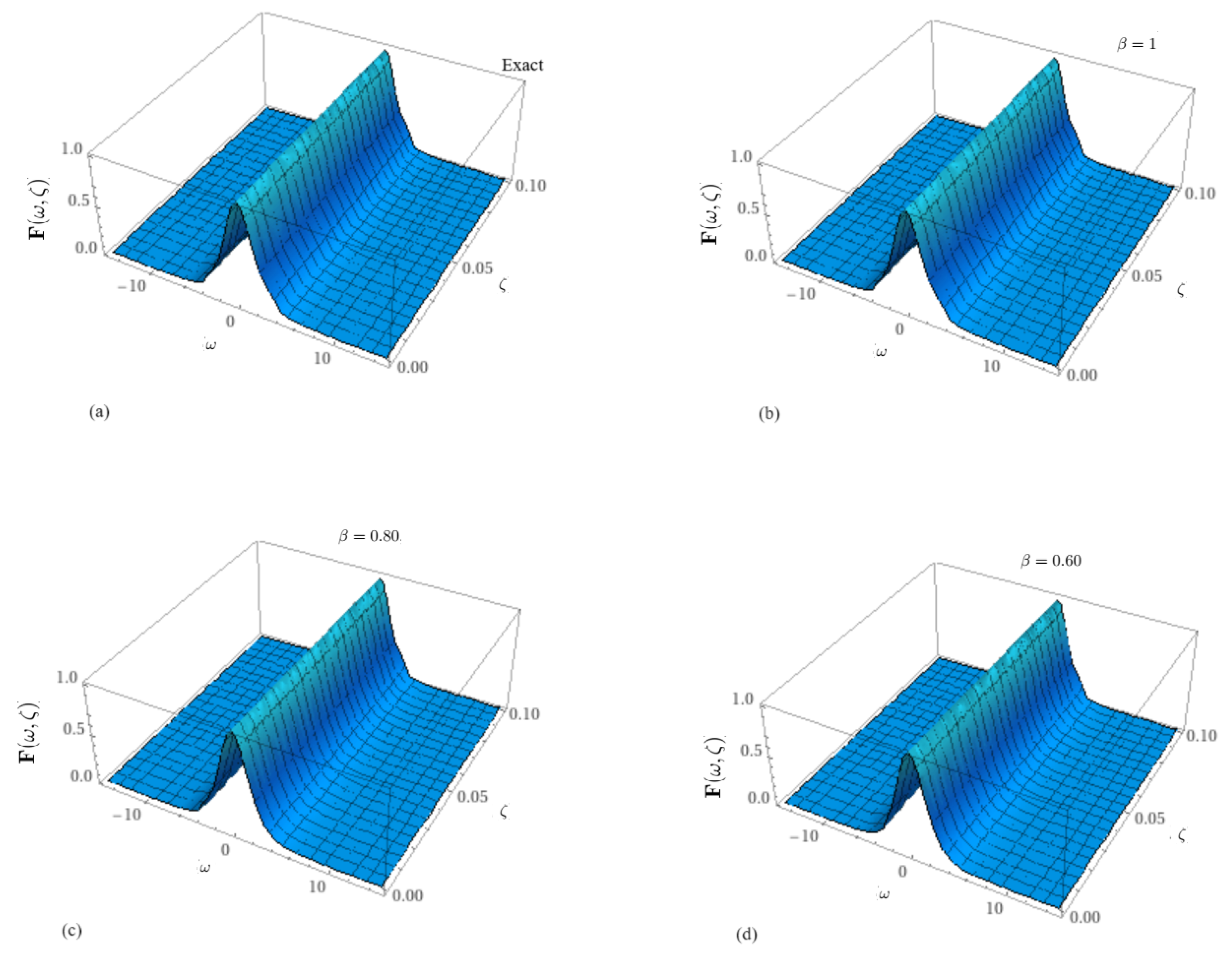
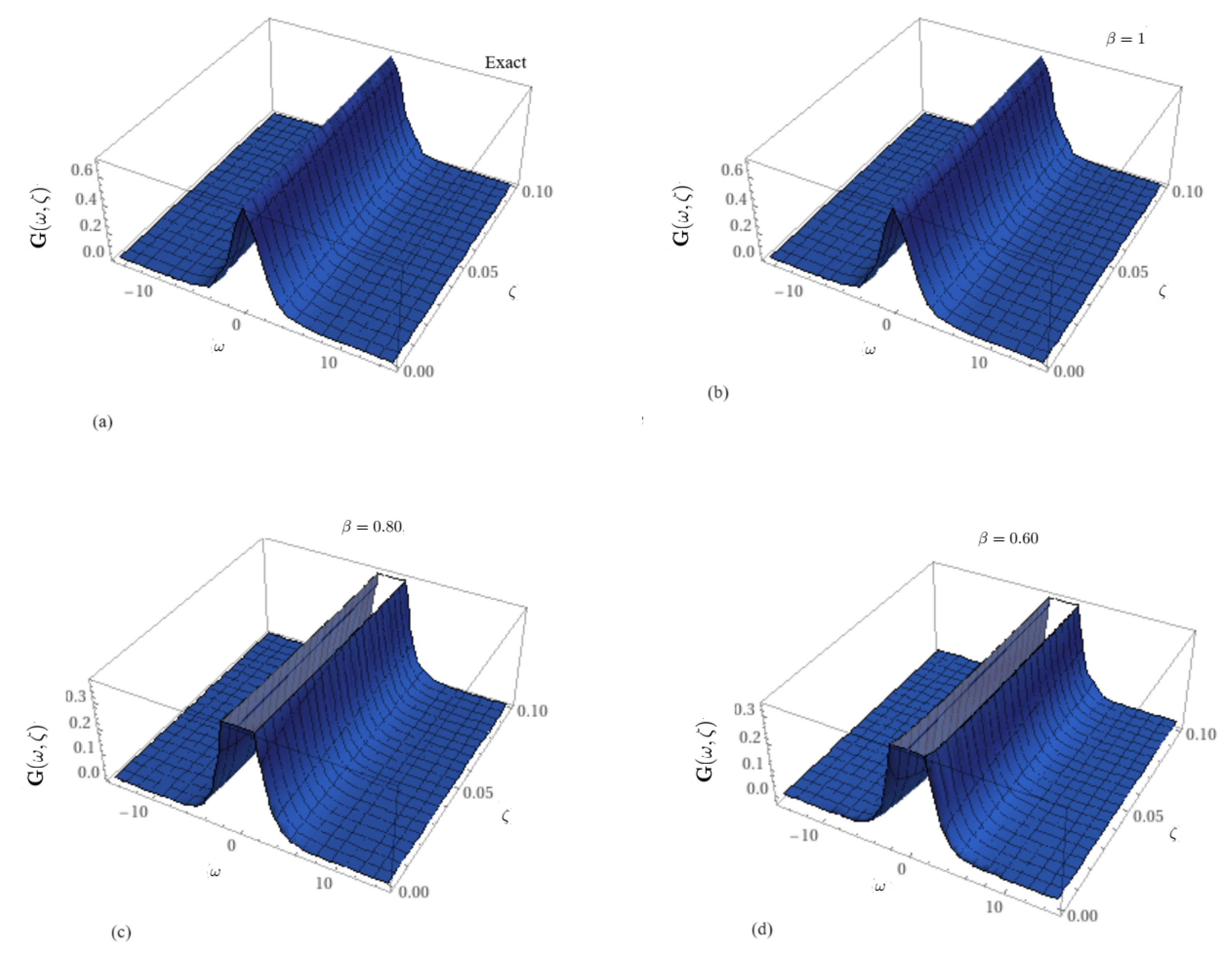
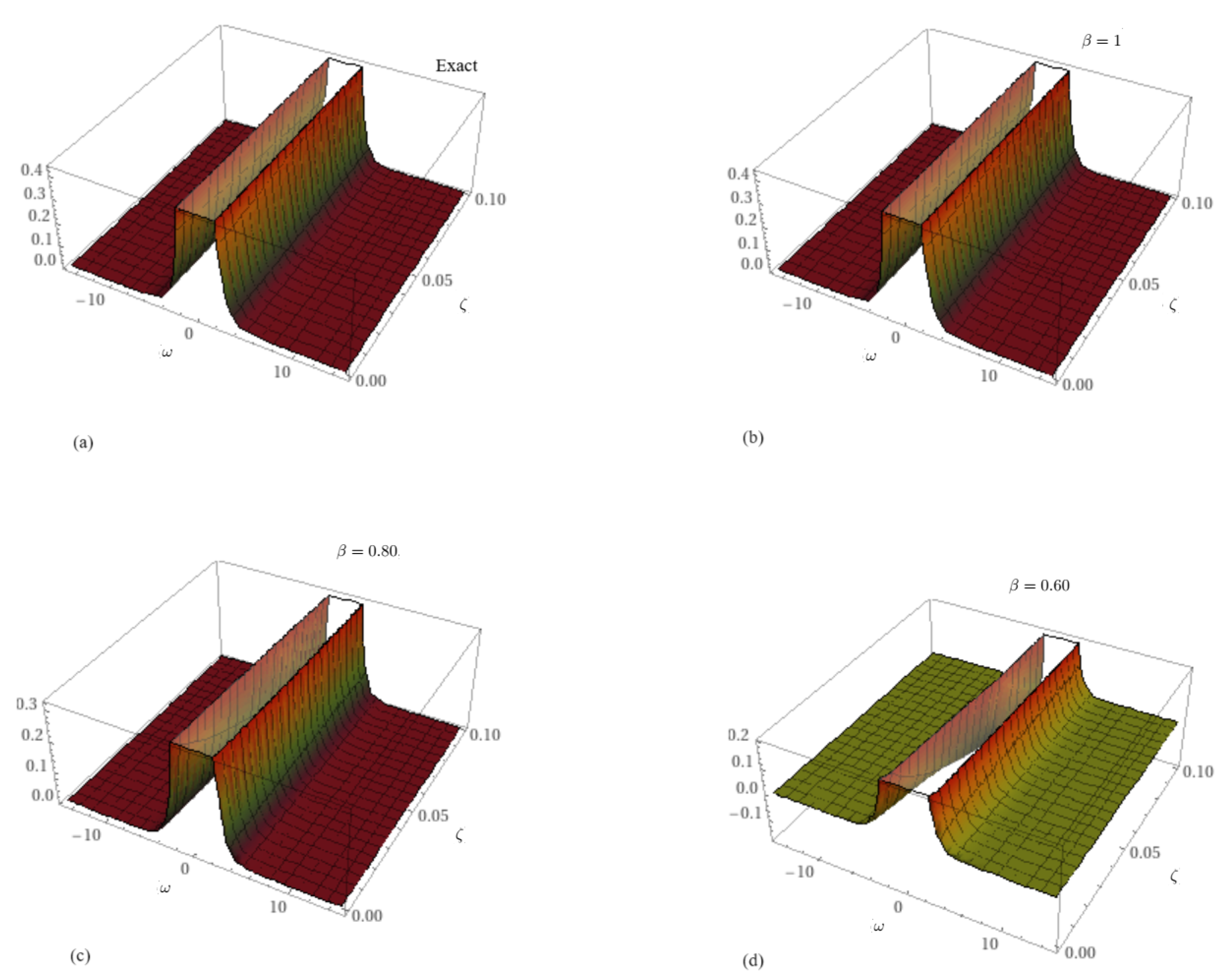
4. Numerical Results

Example 1. 

Let us assume the fractional coupled KdV Equation (1) with $\mathit{a}=-\varsigma ,\mathit{b}=-6\varsigma ,\mathit{c}=2\nu$, $\mathit{d}=-\psi ,$ and $\mathit{e}=3\psi ,$ having the initial guess

$$\mathbf{F}(\omega ,0)=\frac{\xi }{\lambda }{\left(sech\left(\frac{1}{2}\sqrt{\frac{\xi }{\lambda }}\omega \right)\right)}^2,\mathbf{G}(\omega ,0)=\frac{\xi }{\sqrt{2\lambda }}{\left(sech\left(\frac{1}{2}\sqrt{\frac{\xi }{\lambda }}\omega \right)\right)}^2.$$

In terms of NT, we obtain

$$\begin{array}{cc}\hfill & \mathbb{N}\left[D_{\zeta }^{\beta }\mathbf{F}(\omega ,\zeta )\right]=\mathbb{N}[-\lambda {\mathbf{F}}_{\omega \omega \omega }(\omega ,\zeta )-6\lambda \mathbf{F}(\omega ,\zeta ){\mathbf{F}}_{\omega }(\omega ,\zeta )+2\nu \mathbf{G}(\omega ,\zeta ){\mathbf{G}}_{\omega }(\omega ,\zeta )],\hfill \\ \hfill & \mathbb{N}\left[D_{\zeta }^{\beta }\mathbf{G}(\omega ,\zeta )\right]=\mathbb{N}[-\psi {\mathbf{F}}_{\omega \omega \omega }(\omega ,\zeta )-3\psi \mathbf{F}(\omega ,\zeta ){\mathbf{G}}_{\omega }(\omega ,\zeta )].\hfill \end{array}$$

(34)

After, we obtain

$$\begin{array}{cc}\hfill & \frac{1}{{\varsigma }^{\beta }}\mathbb{N}\left[\mathbf{F}(\omega ,\zeta )\right]-{\varsigma }^{2-\beta }\mathbf{F}(\omega ,0)=\mathbb{N}[-\lambda {\mathbf{F}}_{\omega \omega \omega }(\omega ,\zeta )-6\lambda \mathbf{F}(\omega ,\zeta ){\mathbf{F}}_{\omega }(\omega ,\zeta )+2\nu \mathbf{G}(\omega ,\zeta ){\mathbf{G}}_{\omega }(\omega ,\zeta )],\hfill \\ \hfill & \frac{1}{{\varsigma }^{\beta }}\mathbb{N}\left[\mathbf{G}(\omega ,\zeta )\right]-{\varsigma }^{2-\beta }\mathbf{F}(\omega ,0)=\mathbb{N}[-\psi {\mathbf{F}}_{\omega \omega \omega }(\omega ,\zeta )-3\psi \mathbf{F}(\omega ,\zeta ){\mathbf{G}}_{\omega }(\omega ,\zeta )],\hfill \end{array}$$

(35)

which simplifies to

$$\begin{array}{cc}\hfill & \mathbb{N}\left[\mathbf{F}(\omega ,\zeta )\right]={\varsigma }^2\left[\frac{\xi }{\lambda }{\left(sech\left(\frac{1}{2}\sqrt{\frac{\xi }{\lambda }}\omega \right)\right)}^2\right]+\frac{\beta (\varsigma -\beta (\varsigma -\beta \left)\right)}{{\varsigma }^2}\mathbb{N}[-\lambda {\mathbf{F}}_{\omega \omega \omega }(\omega ,\zeta )-6\lambda \mathbf{F}(\omega ,\zeta ){\mathbf{F}}_{\omega }(\omega ,\zeta )\hfill \\ \hfill & +2\nu \mathbf{G}(\omega ,\zeta ){\mathbf{G}}_{\omega }(\omega ,\zeta )],\hfill \\ \hfill & \mathbb{N}\left[\mathbf{G}(\omega ,\zeta )\right]={\varsigma }^2\left[\frac{\xi }{\sqrt{2\lambda }}{\left(sech\left(\frac{1}{2}\sqrt{\frac{\xi }{\lambda }}\omega \right)\right)}^2\right]+\frac{\beta (\varsigma -\beta (\varsigma -\beta \left)\right)}{{\varsigma }^2}\mathbb{N}[-\psi {\mathbf{F}}_{\omega \omega \omega }(\omega ,\zeta )-3\psi \mathbf{F}(\omega ,\zeta ){\mathbf{G}}_{\omega }(\omega ,\zeta )],\hfill \end{array}$$

(36)

By operating the inverse NT, we have

$$\begin{array}{cc}\hfill & \mathbf{F}(\omega ,\zeta )=\left[\frac{\xi }{\lambda }{\left(sech\left(\frac{1}{2}\sqrt{\frac{\xi }{\lambda }}\omega \right)\right)}^2\right]\hfill \\ \hfill & +{\mathbb{N}}^{-1}\left[\frac{\beta (\varsigma -\beta (\varsigma -\beta \left)\right)}{{\varsigma }^2}\mathbb{N}\{-\lambda {\mathbf{F}}_{\omega \omega \omega }(\omega ,\zeta )-6\lambda \mathbf{F}(\omega ,\zeta ){\mathbf{F}}_{\omega }(\omega ,\zeta )+2\nu \mathbf{G}(\omega ,\zeta ){\mathbf{G}}_{\omega }(\omega ,\zeta )\}\right],\hfill \\ \hfill & \mathbf{G}(\omega ,\zeta )=\left[\frac{\xi }{\sqrt{2\lambda }}{\left(sech\left(\frac{1}{2}\sqrt{\frac{\xi }{\lambda }}\omega \right)\right)}^2\right]\hfill \\ \hfill & +{\mathbb{N}}^{-1}\left[\frac{\beta (\varsigma -\beta (\varsigma -\beta \left)\right)}{{\varsigma }^2}\mathbb{N}\{-\psi {\mathbf{F}}_{\omega \omega \omega }(\omega ,\zeta )-3\psi \mathbf{F}(\omega ,\zeta ){\mathbf{G}}_{\omega }(\omega ,\zeta )\}\right].\hfill \end{array}$$

(37)

$ND{M}_{CF}$   solution

The solution of $\mathbf{F}(\omega ,\zeta )$ and $\mathbf{G}(\omega ,\zeta )$ are expanded in series form as

$$\mathbf{F}(\omega ,\zeta )=\sum _{l=0}^{\infty }{\mathbf{F}}_l(\omega ,\zeta )and\mathbf{G}(\omega ,\zeta )=\sum _{l=0}^{\infty }{\mathbf{F}}_l(\omega ,\zeta ).$$

(38)

The nonlinear terms according to Adomian polynomials are as follows $\mathbf{F}(\omega ,\zeta ){\mathbf{F}}_{\omega }(\omega ,\zeta )={\sum }_{m=0}^{\infty }{\mathcal{A}}_m$, $\mathbf{G}(\omega ,\zeta ){\mathbf{G}}_{\omega }(\omega ,\zeta )={\sum }_{m=0}^{\infty }{\mathcal{B}}_m$ and $\mathbf{F}(\omega ,\zeta ){\mathbf{G}}_{\omega }(\omega ,\zeta )={\sum }_{m=0}^{\infty }{\mathcal{C}}_m$; now by putting these terms in Equation (37), we obtain

$$\begin{array}{cc}\hfill & \sum _{l=0}^{\infty }{\mathbf{F}}_{l+1}(\omega ,\zeta )=\frac{\xi }{\lambda }{\left(sech\left(\frac{1}{2}\sqrt{\frac{\xi }{\lambda }}\omega \right)\right)}^2\hfill \\ \hfill & +{\mathbb{N}}^{-1}\left[\frac{\beta (\varsigma -\beta (\varsigma -\beta \left)\right)}{{\varsigma }^2}\mathbb{N}\left\{-\lambda {\mathbf{F}}_{\omega \omega \omega }(\omega ,\zeta )-6\lambda \sum _{l=0}^{\infty }{\mathcal{A}}_l+2\nu \sum _{l=0}^{\infty }{\mathcal{B}}_l\right\}\right],\hfill \\ \hfill & \sum _{l=0}^{\infty }{\mathbf{G}}_{l+1}(\omega ,\zeta )=\frac{\xi }{\sqrt{2\lambda }}{\left(sech\left(\frac{1}{2}\sqrt{\frac{\xi }{\lambda }}\omega \right)\right)}^2\hfill \\ \hfill & +{\mathbb{N}}^{-1}\left[\frac{\beta (\varsigma -\beta (\varsigma -\beta \left)\right)}{{\varsigma }^2}\mathbb{N}\left\{-\psi {\mathbf{F}}_{\omega \omega \omega }(\omega ,\zeta )-3\psi \sum _{l=0}^{\infty }{\mathcal{C}}_l\right\}\right].\hfill \end{array}$$

(39)

By equating both sides of Equation (39), we acquire

$$\begin{array}{cc}\hfill & {\mathbf{F}}_0(\omega ,\zeta )=\frac{\xi }{\lambda }{\left(sech\left(\frac{1}{2}\sqrt{\frac{\xi }{\lambda }}\omega \right)\right)}^2,\hfill \\ \hfill & {\mathbf{G}}_0(\omega ,\zeta )=\frac{\xi }{\sqrt{2\lambda }}{\left(sech\left(\frac{1}{2}\sqrt{\frac{\xi }{\lambda }}\omega \right)\right)}^2,\hfill \end{array}$$

$$\begin{array}{cc}\hfill & {\mathbf{F}}_1(\omega ,\zeta )=\left(\frac{1}{2}\xi {\left(\frac{\xi }{\lambda }\right)}^{\frac{3}{2}}\left(7-2\nu +cosh\left(\sqrt{\frac{\xi }{\lambda }}\omega \right)\right){sech}^4\left(\frac{1}{2}\sqrt{\frac{\xi }{\lambda }}\omega \right)tanh\left(\frac{1}{2}\sqrt{\frac{\xi }{\lambda }}\omega \right)\right)\left(\beta (\zeta -1)+1\right),\hfill \\ \hfill & {\mathbf{G}}_1(\omega ,\zeta )=\left(4\sqrt{2}\sqrt{\lambda }\psi {\left(\frac{\xi }{\lambda }\right)}^{\frac{5}{2}}{csch}^3\left(\sqrt{\frac{\xi }{\lambda }}\omega \right){sinh}^4\left(\frac{1}{2}\sqrt{\frac{\xi }{\lambda }}\omega \right)\right)\left(\beta (\zeta -1)+1\right),\hfill \end{array}$$

(40)

Finally, we obtain the analytical solution of $\mathbf{F}(\omega ,\zeta )$ and $\mathbf{G}(\omega ,\zeta )$ as

$$\begin{array}{cc}\hfill \mathbf{F}(\omega ,\zeta )& =\sum _{l=0}^{\infty }{\mathbf{F}}_l(\omega ,\zeta )={\mathbf{F}}_0(\omega ,\zeta )+{\mathbf{F}}_1(\omega ,\zeta )+\cdots ,\hfill \\ \hfill \mathbf{F}(\omega ,\zeta )& =\frac{\xi }{\lambda }{\left(sech\left(\frac{1}{2}\sqrt{\frac{\xi }{\lambda }}\omega \right)\right)}^2+\left(\frac{1}{2}\xi {\left(\frac{\xi }{\lambda }\right)}^{\frac{3}{2}}\left(7-2\nu +cosh\left(\sqrt{\frac{\xi }{\lambda }}\omega \right)\right){sech}^4\left(\frac{1}{2}\sqrt{\frac{\xi }{\lambda }}\omega \right)tanh\left(\frac{1}{2}\sqrt{\frac{\xi }{\lambda }}\omega \right)\right)\hfill \\ \hfill & \left(\beta \right(\zeta -1)+1)+\cdots .\hfill \\ \hfill \mathbf{G}(\omega ,\zeta )& =\sum _{l=0}^{\infty }{\mathbf{G}}_l(\omega ,\zeta )={\mathbf{G}}_0(\omega ,\zeta )+{\mathbf{G}}_1(\omega ,\zeta )+\cdots ,\hfill \\ \hfill \mathbf{G}(\omega ,\zeta )& =\frac{\xi }{\sqrt{2\lambda }}{\left(sech\left(\frac{1}{2}\sqrt{\frac{\xi }{\lambda }}\omega \right)\right)}^2+\left(4\sqrt{2}\sqrt{\lambda }\psi {\left(\frac{\xi }{\lambda }\right)}^{\frac{5}{2}}{csch}^3\left(\sqrt{\frac{\xi }{\lambda }}\omega \right){sinh}^4\left(\frac{1}{2}\sqrt{\frac{\xi }{\lambda }}\omega \right)\right)\left(\beta (\zeta -1)+1\right)+\cdots .\hfill \end{array}$$

(41)

$ND{M}_{ABC}$   solution

The solutions of $\mathbf{F}(\omega ,\zeta )$ and $\mathbf{G}(\omega ,\zeta )$ are expanded in series form as

$$\begin{array}{cc}\hfill & \mathbf{F}(\omega ,\zeta )=\sum _{l=0}^{\infty }{\mathbf{F}}_l(\omega ,\zeta ),\hfill \\ \hfill & \mathbf{G}(\omega ,\zeta )=\sum _{l=0}^{\infty }{\mathbf{G}}_l(\omega ,\zeta ),\hfill \end{array}$$

(42)

The nonlinear terms according to Adomian polynomials are $\mathbf{F}(\omega ,\zeta ){\mathbf{F}}_{\omega }(\omega ,\zeta )={\sum }_{m=0}^{\infty }{\mathcal{A}}_m$, $\mathbf{G}(\omega ,\zeta ){\mathbf{G}}_{\omega }(\omega ,\zeta )={\sum }_{m=0}^{\infty }{\mathcal{B}}_m$ and $\mathbf{F}(\omega ,\zeta ){\mathbf{G}}_{\omega }(\omega ,\zeta )={\sum }_{m=0}^{\infty }{\mathcal{C}}_m$; now by putting these terms in Equation (37), we obtain

$$\begin{array}{cc}\hfill \sum _{l=0}^{\infty }{\mathbf{F}}_{l+1}(\omega ,\zeta )& =\frac{\xi }{\lambda }{\left(sech\left(\frac{1}{2}\sqrt{\frac{\xi }{\lambda }}\omega \right)\right)}^2\hfill \\ \hfill & +{\mathbb{N}}^{-1}\left[\frac{{\kappa }^{\beta }({\varsigma }^{\beta }+\beta ({\kappa }^{\beta }-{\varsigma }^{\beta }))}{{\varsigma }^{2\beta }}\mathbb{N}\left\{-\lambda {\mathbf{F}}_{\omega \omega \omega }(\omega ,\zeta )-6\lambda \sum _{l=0}^{\infty }{\mathcal{A}}_l+2\nu \sum _{l=0}^{\infty }{\mathcal{B}}_l\right\}\right],\hfill \\ \hfill \sum _{l=0}^{\infty }{\mathbf{G}}_{l+1}(\omega ,\zeta )& =\frac{\xi }{\sqrt{2\lambda }}{\left(sech\left(\frac{1}{2}\sqrt{\frac{\xi }{\lambda }}\omega \right)\right)}^2\hfill \\ \hfill & +{\mathbb{N}}^{-1}\left[\frac{{\kappa }^{\beta }({\varsigma }^{\beta }+\beta ({\kappa }^{\beta }-{\varsigma }^{\beta }))}{{\varsigma }^{2\beta }}\mathbb{N}\left\{-\psi {\mathbf{F}}_{\omega \omega \omega }(\omega ,\zeta )-3\psi \sum _{l=0}^{\infty }{\mathcal{C}}_l\right\}\right].\hfill \end{array}$$

(43)

By equating both sides of Equation (43), we acquire

$$\begin{array}{cc}\hfill & {\mathbf{F}}_0(\omega ,\zeta )=\frac{\xi }{\lambda }{\left(sech\left(\frac{1}{2}\sqrt{\frac{\xi }{\lambda }}\omega \right)\right)}^2,\hfill \\ \hfill & {\mathbf{G}}_0(\omega ,\zeta )=\frac{\xi }{\sqrt{2\lambda }}{\left(sech\left(\frac{1}{2}\sqrt{\frac{\xi }{\lambda }}\omega \right)\right)}^2,\hfill \end{array}$$

$$\begin{array}{cc}\hfill & {\mathbf{F}}_1(\omega ,\zeta )=\left(\frac{1}{2}\xi {\left(\frac{\xi }{\lambda }\right)}^{\frac{3}{2}}\left(7-2\nu +cosh\left(\sqrt{\frac{\xi }{\lambda }}\omega \right)\right){sech}^4\left(\frac{1}{2}\sqrt{\frac{\xi }{\lambda }}\omega \right)tanh\left(\frac{1}{2}\sqrt{\frac{\xi }{\lambda }}\omega \right)\right)\left(1-\beta +\frac{\beta {\zeta }^{\beta }}{\Gamma (\beta +1)}\right),\hfill \\ \hfill & {\mathbf{G}}_1(\omega ,\zeta )=\left(4\sqrt{2}\sqrt{\lambda }\psi {\left(\frac{\xi }{\lambda }\right)}^{\frac{5}{2}}{csch}^3\left(\sqrt{\frac{\xi }{\lambda }}\omega \right){sinh}^4\left(\frac{1}{2}\sqrt{\frac{\xi }{\lambda }}\omega \right)\right)\left(1-\beta +\frac{\beta {\zeta }^{\beta }}{\Gamma (\beta +1)}\right),\hfill \end{array}$$

(44)

Finally, we obtain the analytical solution of $\mathbf{F}(\omega ,\zeta )$ and $\mathbf{G}(\omega ,\zeta )$ as

$$\begin{array}{cc}\hfill \mathbf{F}(\omega ,\zeta )& =\sum _{l=0}^{\infty }{\mathbf{F}}_l(\omega ,\zeta )={\mathbf{F}}_0(\omega ,\zeta )+{\mathbf{F}}_1(\omega ,\zeta )+\cdots ,\hfill \\ \hfill \mathbf{F}(\omega ,\zeta )& =\frac{\xi }{\lambda }{\left(sech\left(\frac{1}{2}\sqrt{\frac{\xi }{\lambda }}\omega \right)\right)}^2+\left(\frac{1}{2}\xi {\left(\frac{\xi }{\lambda }\right)}^{\frac{3}{2}}\left(7-2\nu +cosh\left(\sqrt{\frac{\xi }{\lambda }}\omega \right)\right){sech}^4\left(\frac{1}{2}\sqrt{\frac{\xi }{\lambda }}\omega \right)tanh\left(\frac{1}{2}\sqrt{\frac{\xi }{\lambda }}\omega \right)\right)\hfill \\ \hfill & \left(1-\beta +\frac{\beta {\zeta }^{\beta }}{\Gamma (\beta +1)}\right)+\cdots \hfill \\ \hfill \mathbf{G}(\omega ,\zeta )& =\sum _{l=0}^{\infty }{\mathbf{G}}_l(\omega ,\zeta )={\mathbf{G}}_0(\omega ,\zeta )+{\mathbf{G}}_1(\omega ,\zeta )+\cdots ,\hfill \\ \hfill \mathbf{G}(\omega ,\zeta )& =\frac{\xi }{\sqrt{2\lambda }}{\left(sech\left(\frac{1}{2}\sqrt{\frac{\xi }{\lambda }}\omega \right)\right)}^2+\left(4\sqrt{2}\sqrt{\lambda }\psi {\left(\frac{\xi }{\lambda }\right)}^{\frac{5}{2}}{csch}^3\left(\sqrt{\frac{\xi }{\lambda }}\omega \right){sinh}^4\left(\frac{1}{2}\sqrt{\frac{\xi }{\lambda }}\omega \right)\right)\left(1-\beta +\frac{\beta {\zeta }^{\beta }}{\Gamma (\beta +1)}\right)+\cdots \hfill \end{array}$$

(45)

At $\beta =1$, we obtain the exact solution as

$$\begin{array}{cc}\hfill & \mathbf{F}(\omega ,\zeta )=\frac{\xi }{\lambda }{\left(sech\left(\frac{1}{2}\sqrt{\frac{\xi }{\lambda }}(\omega -\xi \zeta )\right)\right)}^2,\hfill \\ \hfill & \mathbf{G}(\omega ,\zeta )=\frac{\xi }{\sqrt{2\lambda }}{\left(sech\left(\frac{1}{2}\sqrt{\frac{\xi }{\lambda }}(\omega -\xi \zeta )\right)\right)}^2,\hfill \end{array}$$

(46)

Example 2. 

Let us assume fractional coupled KdV Equation (1) with $\mathit{a}=-1,\mathit{b}=-6,\mathit{c}=3$, $\mathit{d}=-1$, and $\mathit{e}=3,$ having initial guess

$$\mathbf{F}(\omega ,0)=\frac{4{\sigma }^2{e}^{\sigma \omega }}{{(1+e^{\sigma \omega })}^2},\mathbf{G}(\omega ,0)=\frac{4{\sigma }^2{e}^{\sigma \omega }}{{(1+e^{\sigma \omega })}^2}.$$

In terms of NT, we obtain

$$\begin{array}{cc}\hfill & \mathbb{N}\left[D_{\zeta }^{\beta }\mathbf{F}(\omega ,\zeta )\right]=\mathbb{N}\left[-{\mathbf{F}}_{\omega \omega \omega }(\omega ,\zeta )-6\mathbf{F}(\omega ,\zeta ){\mathbf{F}}_{\omega }(\omega ,\zeta )+3\mathbf{G}(\omega ,\zeta ){\mathbf{G}}_{\omega }(\omega ,\zeta )\right],\hfill \\ \hfill & \mathbb{N}\left[D_{\zeta }^{\beta }\mathbf{G}(\omega ,\zeta )\right]=\mathbb{N}\left[-{\mathbf{F}}_{\omega \omega \omega }(\omega ,\zeta )-3\mathbf{F}(\omega ,\zeta ){\mathbf{G}}_{\omega }(\omega ,\zeta )\right].\hfill \end{array}$$

(47)

After, we obtain

$$\begin{array}{cc}\hfill & \frac{1}{{\varsigma }^{\beta }}\mathbb{N}\left[\mathbf{F}(\omega ,\zeta )\right]-{\varsigma }^{2-\beta }\mathbf{F}(\omega ,0)=\mathbb{N}\left[-{\mathbf{F}}_{\omega \omega \omega }(\omega ,\zeta )-6\mathbf{F}(\omega ,\zeta ){\mathbf{F}}_{\omega }(\omega ,\zeta )+3\mathbf{G}(\omega ,\zeta ){\mathbf{G}}_{\omega }(\omega ,\zeta )\right],\hfill \\ \hfill & \frac{1}{{\varsigma }^{\beta }}\mathbb{N}\left[\mathbf{G}(\omega ,\zeta )\right]-{\varsigma }^{2-\beta }\mathbf{F}(\omega ,0)=\mathbb{N}\left[-{\mathbf{F}}_{\omega \omega \omega }(\omega ,\zeta )-3\mathbf{F}(\omega ,\zeta ){\mathbf{G}}_{\omega }(\omega ,\zeta )\right],\hfill \end{array}$$

(48)

which simplifies to

$$\begin{array}{cc}\hfill & \mathbb{N}\left[\mathbf{F}(\omega ,\zeta )\right]={\varsigma }^2\left[\frac{4{\beta }^2{e}^{\beta \omega }}{{(1+e^{\beta \omega })}^2}\right]+\frac{\beta (\varsigma -\beta (\varsigma -\beta \left)\right)}{{\varsigma }^2}\mathbb{N}\left[-{\mathbf{F}}_{\omega \omega \omega }(\omega ,\zeta )-6\mathbf{F}(\omega ,\zeta ){\mathbf{F}}_{\omega }(\omega ,\zeta )+3\mathbf{G}(\omega ,\zeta ){\mathbf{G}}_{\omega }(\omega ,\zeta )\right],\hfill \\ \hfill & \mathbb{N}\left[\mathbf{G}(\omega ,\zeta )\right]={\varsigma }^2\left[\frac{4{\beta }^2{e}^{\beta \omega }}{{(1+e^{\beta \omega })}^2}\right]+\frac{\beta (\varsigma -\beta (\varsigma -\beta \left)\right)}{{\varsigma }^2}\mathbb{N}\left[-{\mathbf{F}}_{\omega \omega \omega }(\omega ,\zeta )-3\mathbf{F}(\omega ,\zeta ){\mathbf{G}}_{\omega }(\omega ,\zeta )\right].\hfill \end{array}$$

(49)

By operating the inverse NT, we have

$$\begin{array}{cc}\hfill & \mathbf{F}(\omega ,\zeta )=\left[\frac{4{\sigma }^2{e}^{\sigma \omega }}{{(1+e^{\sigma \omega })}^2}\right]\hfill \\ \hfill & +{\mathbb{N}}^{-1}\left[\frac{\beta (\varsigma -\beta (\varsigma -\beta \left)\right)}{{\varsigma }^2}\mathbb{N}\{-{\mathbf{F}}_{\omega \omega \omega }(\omega ,\zeta )-6\mathbf{F}(\omega ,\zeta ){\mathbf{F}}_{\omega }(\omega ,\zeta )+3\mathbf{G}(\omega ,\zeta ){\mathbf{G}}_{\omega }(\omega ,\zeta )\right]\},\hfill \\ \hfill & \mathbf{G}(\omega ,\zeta )=\left[\frac{4{\sigma }^2{e}^{\sigma \omega }}{{(1+e^{\sigma \omega })}^2}\right]\hfill \\ \hfill & +{\mathbb{N}}^{-1}\left[\frac{\beta (\varsigma -\beta (\varsigma -\beta \left)\right)}{{\varsigma }^2}\mathbb{N}\{-{\mathbf{F}}_{\omega \omega \omega }(\omega ,\zeta )-3\mathbf{F}(\omega ,\zeta ){\mathbf{G}}_{\omega }(\omega ,\zeta )\}\right],\hfill \end{array}$$

(50)

$ND{M}_{CF}$   solution

The solution of $\mathbf{F}(\omega ,\zeta )$ and $\mathbf{G}(\omega ,\zeta )$ are expanded in series form as

$$\mathbf{F}(\omega ,\zeta )=\sum _{l=0}^{\infty }{\mathbf{F}}_l(\omega ,\zeta )and\mathbf{G}(\omega ,\zeta )=\sum _{l=0}^{\infty }{\mathbf{F}}_l(\omega ,\zeta ).$$

(51)

The nonlinear terms according to Adomian polynomials are $\mathbf{F}(\omega ,\zeta ){\mathbf{F}}_{\omega }(\omega ,\zeta )={\sum }_{m=0}^{\infty }{\mathcal{A}}_m$, $\mathbf{G}(\omega ,\zeta ){\mathbf{G}}_{\omega }(\omega ,\zeta )={\sum }_{m=0}^{\infty }{\mathcal{B}}_m$ and $\mathbf{F}(\omega ,\zeta ){\mathbf{G}}_{\omega }(\omega ,\zeta )={\sum }_{m=0}^{\infty }{\mathcal{C}}_m$; now by putting these terms in Equation (50), we obtain

$$\begin{array}{cc}\hfill & \sum _{l=0}^{\infty }{\mathbf{F}}_{l+1}(\omega ,\zeta )=\frac{4{\sigma }^2{e}^{\sigma \omega }}{{(1+e^{\sigma \omega })}^2}\hfill \\ \hfill & +{\mathbb{N}}^{-1}\left[\frac{\beta (\varsigma -\beta (\varsigma -\beta \left)\right)}{{\varsigma }^2}\mathbb{N}\left\{-{\mathbf{F}}_{\omega \omega \omega }(\omega ,\zeta )-6\lambda \sum _{l=0}^{\infty }{\mathcal{A}}_l+3\nu \sum _{l=0}^{\infty }{\mathcal{B}}_l\right\}\right],\hfill \\ \hfill & \sum _{l=0}^{\infty }{\mathbf{G}}_{l+1}(\omega ,\zeta )=\frac{4{\sigma }^2{e}^{\sigma \omega }}{{(1+e^{\sigma \omega })}^2}\hfill \\ \hfill & +{\mathbb{N}}^{-1}\left[\frac{\beta (\varsigma -\beta (\varsigma -\beta \left)\right)}{{\varsigma }^2}\mathbb{N}\left\{-{\mathbf{F}}_{\omega \omega \omega }(\omega ,\zeta )-3\sum _{l=0}^{\infty }{\mathcal{C}}_l\right\}\right].\hfill \end{array}$$

(52)

By equating both sides of Equation (52), we acquire

$$\begin{array}{cc}\hfill & {\mathbf{F}}_0(\omega ,\zeta )=\frac{4{\sigma }^2{e}^{\sigma \omega }}{{(1+e^{\sigma \omega })}^2},\hfill \\ \hfill & {\mathbf{G}}_0(\omega ,\zeta )=\frac{4{\sigma }^2{e}^{\sigma \omega }}{{(1+e^{\sigma \omega })}^2},\hfill \end{array}$$

$$\begin{array}{cc}\hfill & {\mathbf{F}}_1(\omega ,\zeta )=\left(\frac{4{\beta }^5{e}^{\beta \omega }(-1+e^{\beta \omega })}{{(1+e^{\beta \omega })}^3}\right)\left(\beta (\zeta -1)+1\right),\hfill \\ \hfill & {\mathbf{G}}_1(\omega ,\zeta )=\left(\frac{4{\beta }^5{e}^{\beta \omega }(-1+e^{\beta \omega })}{{(1+e^{\beta \omega })}^3}\right)\left(\beta (\zeta -1)+1\right).\hfill \end{array}$$

(53)

Finally, we obtain the analytical solution of $\mathbf{F}(\omega ,\zeta )$ and $\mathbf{G}(\omega ,\zeta )$ as

$$\begin{array}{cc}\hfill \mathbf{F}(\omega ,\zeta )& =\sum _{l=0}^{\infty }{\mathbf{F}}_l(\omega ,\zeta )={\mathbf{F}}_0(\omega ,\zeta )+{\mathbf{F}}_1(\omega ,\zeta )+\cdots ,\hfill \\ \hfill \mathbf{F}(\omega ,\zeta )& =\frac{4{\sigma }^2{e}^{\sigma \omega }}{{(1+e^{\sigma \omega })}^2}+\left(\frac{4{\beta }^5{e}^{\beta \omega }(-1+e^{\beta \omega })}{{(1+e^{\beta \omega })}^3}\right)\left(\beta (\zeta -1)+1\right)+\cdots .\hfill \\ \hfill \mathbf{G}(\omega ,\zeta )& =\sum _{l=0}^{\infty }{\mathbf{G}}_l(\omega ,\zeta )={\mathbf{G}}_0(\omega ,\zeta )+{\mathbf{G}}_1(\omega ,\zeta )+\cdots ,\hfill \\ \hfill \mathbf{G}(\omega ,\zeta )& =\frac{4{\sigma }^2{e}^{\sigma \omega }}{{(1+e^{\sigma \omega })}^2}+\left(\frac{4{\beta }^5{e}^{\beta \omega }(-1+e^{\beta \omega })}{{(1+e^{\beta \omega })}^3}\right)\left(\beta (\zeta -1)+1\right)+\cdots .\hfill \end{array}$$

(54)

$ND{M}_{ABC}$   solution

The solutions of $\mathbf{F}(\omega ,\zeta )$ and $\mathbf{G}(\omega ,\zeta )$ are expanded in series form as

$$\begin{array}{cc}\hfill & \mathbf{F}(\omega ,\zeta )=\sum _{l=0}^{\infty }{\mathbf{F}}_l(\omega ,\zeta ),\hfill \\ \hfill & \mathbf{G}(\omega ,\zeta )=\sum _{l=0}^{\infty }{\mathbf{F}}_l(\omega ,\zeta ),\hfill \end{array}$$

(55)

The nonlinear terms according to Adomian polynomials are $\mathbf{F}(\omega ,\zeta ){\mathbf{F}}_{\omega }(\omega ,\zeta )={\sum }_{m=0}^{\infty }{\mathcal{A}}_m$, $\mathbf{G}(\omega ,\zeta ){\mathbf{G}}_{\omega }(\omega ,\zeta )={\sum }_{m=0}^{\infty }{\mathcal{B}}_m$ and $\mathbf{F}(\omega ,\zeta ){\mathbf{G}}_{\omega }(\omega ,\zeta )={\sum }_{m=0}^{\infty }{\mathcal{C}}_m$; now by putting these terms in Equation (50), we obtain

$$\begin{array}{cc}\hfill \sum _{l=0}^{\infty }{\mathbf{F}}_{l+1}(\omega ,\zeta )& =\frac{4{\sigma }^2{e}^{\sigma \omega }}{{(1+e^{\sigma \omega })}^2}\hfill \\ \hfill & +{\mathbb{N}}^{-1}\left[\frac{{\kappa }^{\beta }({\varsigma }^{\beta }+\beta ({\kappa }^{\beta }-{\varsigma }^{\beta }))}{{\varsigma }^{2\beta }}\mathbb{N}\left\{-{\mathbf{F}}_{\omega \omega \omega }(\omega ,\zeta )-6\lambda \sum _{l=0}^{\infty }{\mathcal{A}}_l+3\nu \sum _{l=0}^{\infty }{\mathcal{B}}_l\right\}\right],\hfill \\ \hfill \sum _{l=0}^{\infty }{\mathbf{G}}_{l+1}(\omega ,\zeta )& =\frac{4{\sigma }^2{e}^{\sigma \omega }}{{(1+e^{\sigma \omega })}^2}\hfill \\ \hfill & +{\mathbb{N}}^{-1}\left[\frac{{\kappa }^{\beta }({\varsigma }^{\beta }+\beta ({\kappa }^{\beta }-{\varsigma }^{\beta }))}{{\varsigma }^{2\beta }}\mathbb{N}\left\{-{\mathbf{F}}_{\omega \omega \omega }(\omega ,\zeta )-3\sum _{l=0}^{\infty }{\mathcal{C}}_l\right\}\right].\hfill \end{array}$$

(56)

By equating both sides of Equation (56), we acquire

$$\begin{array}{cc}\hfill & {\mathbf{F}}_0(\omega ,\zeta )=\frac{4{\sigma }^2{e}^{\sigma \omega }}{{(1+e^{\sigma \omega })}^2},\hfill \\ \hfill & {\mathbf{G}}_0(\omega ,\zeta )=\frac{4{\sigma }^2{e}^{\sigma \omega }}{{(1+e^{\sigma \omega })}^2},\hfill \end{array}$$

$$\begin{array}{cc}\hfill & {\mathbf{F}}_1(\omega ,\zeta )=\left(\frac{4{\beta }^5{e}^{\beta \omega }(-1+e^{\beta \omega })}{{(1+e^{\beta \omega })}^3}\right)\left(1-\beta +\frac{\beta {\zeta }^{\beta }}{\Gamma (\beta +1)}\right),\hfill \\ \hfill & {\mathbf{G}}_1(\omega ,\zeta )=\left(\frac{4{\beta }^5{e}^{\beta \omega }(-1+e^{\beta \omega })}{{(1+e^{\beta \omega })}^3}\right)\left(1-\beta +\frac{\beta {\zeta }^{\beta }}{\Gamma (\beta +1)}\right),\hfill \end{array}$$

(57)

Finally, we obtain the analytical solution of $\mathbf{F}(\omega ,\zeta )$ and $\mathbf{G}(\omega ,\zeta )$ as

$$\begin{array}{cc}\hfill \mathbf{F}(\omega ,\zeta )& =\sum _{l=0}^{\infty }{\mathbf{F}}_l(\omega ,\zeta )={\mathbf{F}}_0(\omega ,\zeta )+{\mathbf{F}}_1(\omega ,\zeta )+\cdots ,\hfill \\ \hfill \mathbf{F}(\omega ,\zeta )& =\frac{4{\sigma }^2{e}^{\sigma \omega }}{{(1+e^{\sigma \omega })}^2}+\left(\frac{4{\beta }^5{e}^{\beta \omega }(-1+e^{\beta \omega })}{{(1+e^{\beta \omega })}^3}\right)\left(1-\beta +\frac{\beta {\zeta }^{\beta }}{\Gamma (\beta +1)}\right)+\cdots \hfill \\ \hfill \mathbf{G}(\omega ,\zeta )& =\sum _{l=0}^{\infty }{\mathbf{G}}_l(\omega ,\zeta )={\mathbf{G}}_0(\omega ,\zeta )+{\mathbf{G}}_1(\omega ,\zeta )+\cdots ,\hfill \\ \hfill \mathbf{G}(\omega ,\zeta )& =\frac{4{\sigma }^2{e}^{\sigma \omega }}{{(1+e^{\sigma \omega })}^2}+\left(\frac{4{\beta }^5{e}^{\beta \omega }(-1+e^{\beta \omega })}{{(1+e^{\beta \omega })}^3}\right)\left(1-\beta +\frac{\beta {\zeta }^{\beta }}{\Gamma (\beta +1)}\right)+\cdots \hfill \end{array}$$

(58)

At $\beta =1$, we obtain the exact solution as

$$\begin{array}{cc}\hfill & \mathbf{F}(\omega ,\zeta )=\mathbf{G}(\omega ,\zeta )=\frac{4{\sigma }^2{e}^{\sigma (\omega -{\sigma }^2\zeta )}}{{(1+e^{\sigma (\omega -{\sigma }^2\zeta )})}^2}.\hfill \end{array}$$

(59)

5. Results Discussion

The graphical and numerical analysis presented in this section offers valuable insights into the behavior and accuracy of our proposed solution method for the coupled Korteweg–de Vries (KdV) equations using non-singular kernel operators in conjunction with the natural transform across varying values of the fractional parameter $\beta$.

In Figure 1, we depict the behavior of the exact solution of $\mathbf{F}(\omega ,\zeta )$ alongside our approach’s solutions at different values of $\beta$, including $\beta =1$, $\beta =0.80$, and $\beta =0.60$ of $\mathbf{F}(\omega ,\zeta )$ for Example 1. These graphs allow us to visually compare how well our method approximates the exact solution as $\beta$ varies. Our approach evidently provides a reasonably accurate representation of the exact solution, with deviations becoming more noticeable as $\beta$ decreases.

Figure 2 follows a similar pattern as Figure 1 but for $\mathbf{G}(\omega ,\zeta )$. We observe the behavior of the exact solution and our approach’s solutions at $\beta =1$, $\beta =0.80$, and $\beta =0.60$ of $\mathbf{G}(\omega ,\zeta )$. Again, these visualizations enable us to assess the performance of our method in approximating the exact solution. As $\beta$ decreases, some deviation from the exact solution is observed, but our approach remains a promising approximation method.

We continue our analysis in Figure 3, but now for Example 2. We explore the behavior of the exact solution and our approach’s solutions at different $\beta$ values, including $\beta =1$, $\beta =0.80$, and $\beta =0.60$ of $\mathbf{F}(\omega ,\zeta )$ and $\mathbf{G}(\omega ,\zeta )$. These graphs highlight the ability of our method to adapt to varying fractional parameters and provide reasonable approximations of the exact solution.

Table 1. Comparison between the proposed method and exact solutions for $\mathbf{F}(\omega ,\zeta )$ at numerous orders of $\beta$ of Example 1.

$(\mathit{\omega },\mathit{\zeta })$	Solution at $\mathit{\beta }=$ 0.6	Solution at $\mathit{\beta }=$ 0.8	$\left({\mathit{NTDM}}_{\mathit{ABC}}\right)$ at $\mathit{\beta }=$ 1	$\left({\mathit{NTDM}}_{\mathit{CF}}\right)$ at $\mathit{\beta }=$ 1	Exact Solution
(0.2, 0. 001)	0.99027100	0.99020853	0.99016496	0.99016496	0.99016472
(0.4, 0.001)	0.96143650	0.96131642	0.96123266	0.96123266	0.96123245
(0.6, 0.001)	0.91569002	0.91552126	0.91540355	0.91540355	0.91540338
(0.8, 0.001)	0.85631323	0.85610742	0.85596388	0.85596388	0.85596376
(0.2, 0.003)	0.99061654	0.99047022	0.99036232	0.99036232	0.99036016
(0.4, 0.003)	0.96210071	0.96181945	0.96161204	0.96161204	0.96161013
(0.6, 0.003)	0.91662353	0.91622824	0.91593673	0.91593673	0.91593519
(0.8, 0.003)	0.85745160	0.85696957	0.85661408	0.85661408	0.85661298
(0.2, 0.005)	0.99093770	0.99072253	0.99055968	0.99055968	0.99055367
(0.4, 0.005)	0.96271807	0.96230447	0.96199141	0.96199141	0.96198610
(0.6, 0.005)	0.91749119	0.91690990	0.91646991	0.91646991	0.91646564
(0.8, 0.005)	0.85850969	0.85780082	0.85726428	0.85726428	0.85726123

and

Table 2. Comparison between the exact solution and our solution for $\mathbf{G}(\omega ,\zeta )$ at numerous orders of $\beta$ of Example 1.

$(\mathit{\omega },\mathit{\zeta })$	Solution at $\mathit{\beta }=$ 0.6	Solution at $\mathit{\beta }=$ 0.8	$\left({\mathit{NTDM}}_{\mathit{ABC}}\right)$ at $\mathit{\beta }=$ 1	$\left(\mathit{N}\mathit{T}\mathit{D}{\mathit{M}}_{\mathit{C}\mathit{F}}\right)$ at $\mathit{\beta }=$ 1	Exact Solution
(0.2, 0.001)	0.70051685	0.70038434	0.70029191	0.70029191	0.70015219
(0.4, 0.001)	0.68039479	0.68014006	0.67996239	0.67996239	0.67969398
(0.6, 0.001)	0.64827277	0.64791477	0.64766507	0.64766507	0.64728793
(0.8, 0.001)	0.60645870	0.60602213	0.60571762	0.60571762	0.60525778
(0.2, 0.003)	0.70124984	0.70093946	0.70071057	0.70071057	0.70029038
(0.4, 0.003)	0.68180379	0.68120716	0.68076716	0.68076716	0.67996104
(0.6, 0.003)	0.65025304	0.64941451	0.64879612	0.64879612	0.64766398
(0.8, 0.003)	0.60887356	0.60785100	0.60709690	0.60709690	0.60571685
(0.2, 0.005)	0.70193113	0.70147470	0.70112922	0.70112922	0.70042721
(0.4, 0.005)	0.68311342	0.68223603	0.68157193	0.68157193	0.68022689
(0.6, 0.005)	0.65209362	0.65086052	0.64992717	0.64992717	0.64803907
(0.8, 0.005)	0.61111810	0.60961437	0.60847618	0.60847618	0.60617523

present a quantitative analysis of the accuracy of our method by comparing the results of our approach with the exact solutions for $\mathbf{F}(\omega ,\zeta )$ and $\mathbf{G}(\omega ,\zeta )$ at various orders of $\beta$. The comparison between

Table 3. Error comparison between our solution for $\mathbf{F}(\omega ,\zeta )$ and the results obtained in [50] of Example 1.

$\mathit{\omega }$	$\mathit{\zeta }$	Error of [50]	$\left({\mathit{NTDM}}_{\mathit{ABC}}\right)$ Error	$\left({\mathit{NTDM}}_{\mathit{CF}}\right)$ Error
−10	0.1	2.99039$\times {10}^{-8}$	1.6125789000$\times {10}^{-8}$	1.6125789000$\times {10}^{-8}$
−10	0.2	2.33335$\times {10}^{-7}$	6.1317061000$\times {10}^{-8}$	6.1317061000$\times {10}^{-8}$
−5	0.1	3.96592$\times {10}^{-6}$	4.3621745000$\times {10}^{-7}$	4.3621745000$\times {10}^{-7}$
−5	0.2	0.0000338049	1.6588950200$\times {10}^{-7}$	1.6588950200$\times {10}^{-7}$
5	0.1	3.97592$\times {10}^{-6}$	4.8456311000$\times {10}^{-7}$	4.8456311000$\times {10}^{-7}$
5	0.2	0.0000378049	2.0470878500$\times {10}^{-7}$	2.0470878500$\times {10}^{-7}$
10	0.1	2.96039$\times {10}^{-8}$	1.7918592000$\times {10}^{-8}$	1.7918592000$\times {10}^{-8}$
10	0.2	2.37335$\times {10}^{-7}$	7.5713342000$\times {10}^{-8}$	7.5713342000$\times {10}^{-8}$

and

Table 4. Error comparison between our solution for $\mathbf{G}(\omega ,\zeta )$ and the results obtained in [50] of Example 1.

$\mathit{\omega }$	$\mathit{\zeta }$	Error of [50]	${\mathit{NTDM}}_{\mathit{ABC}}$ Error	${\mathit{NTDM}}_{\mathit{CF}}$ Error
−10	0.1	2.18624$\times {10}^{-8}$	3.8791346860$\times {10}^{-9}$	3.8791346860$\times {10}^{-9}$
−10	0.2	1.64872 $\times {10}^{-7}$	7.8076524100$\times {10}^{-9}$	7.8076524100$\times {10}^{-9}$
−5	0.1	2.88312$\times {10}^{-6}$	2.7814445650$\times {10}^{-7}$	2.7814445650$\times {10}^{-7}$
−5	0.2	0.0000287824	5.5982968930$\times {10}^{-7}$	5.5982968930$\times {10}^{-7}$
5	0.1	2.98312 $\times {10}^{-6}$	2.7371653580$\times {10}^{-7}$	2.7371653580$\times {10}^{-7}$
5	0.2	0.0000247824	5.4189576320$\times {10}^{-7}$	5.4189576320$\times {10}^{-7}$
10	0.1	2.09624 $\times {10}^{-8}$	3.8173772900$\times {10}^{-9}$	3.8173772900$\times {10}^{-9}$
10	0.2	1.72872 $\times {10}^{-7}$	7.5575220640$\times {10}^{-9}$	7.5575220640$\times {10}^{-9}$

shows that the solutions obtained in this paper are more accurate than those obtained in [50].

Table 5. Comparison between the exact solution and our solution for $\mathbf{F}(\omega ,\zeta )$ and $\mathbf{G}(\omega ,\zeta )$ at numerous orders of $\beta$ of Example 2.

$(\mathit{\omega },\mathit{\zeta })$	Solution at $\mathit{\beta }=$ 0.6	Solution at $\mathit{\beta }=$ 0.8	$\left({\mathit{NTDM}}_{\mathit{ABC}}\right)$ at $\mathit{\beta }=$ 1	$\left({\mathit{NTDM}}_{\mathit{CF}}\right)$ at $\mathit{\beta }=$ 1	Exact Solution
(0.2, 0.001)	0.99027100	0.99020853	0.99016496	0.99016496	0.99016472
(0.4, 0.001)	0.96143650	0.96131642	0.96123266	0.96123266	0.96123245
(0.6, 0.001)	0.91569002	0.91552126	0.91540355	0.91540355	0.91540338
(0.8, 0.001)	0.85631323	0.85610742	0.85596388	0.85596388	0.85596376
(0.2, 0.003)	0.99061654	0.99047022	0.99036232	0.99036232	0.99036016
(0.4, 0.003)	0.96210071	0.96181945	0.96161204	0.96161204	0.96161013
(0.6, 0.003)	0.91662353	0.91622824	0.91593673	0.91593673	0.91593519
(0.8, 0.003)	0.85745160	0.85696957	0.85661408	0.85661408	0.85661298
(0.2, 0.005)	0.99093770	0.99072253	0.99055968	0.99055968	0.99055367
(0.4, 0.005)	0.96271807	0.96230447	0.96199141	0.96199141	0.96198610
(0.6, 0.005)	0.91749119	0.91690990	0.91646991	0.91646991	0.91646564
(0.8, 0.005)	0.85850969	0.85780082	0.85726428	0.85726428	0.85726123

presents a quantitative analysis of the accuracy of our method by comparing the results of our approach with the exact solutions for $\mathbf{F}(\omega ,\zeta )$ and $\mathbf{G}(\omega ,\zeta )$ at various orders of $\beta$. These tables offer numerical evidence of our method’s performance and consistency across different orders of $\beta$.

In summary, our graphical and numerical analysis demonstrates the effectiveness of our proposed method in approximating the solutions of coupled KdV equations via non-singular kernel operators within the framework of the natural transform. While some deviation from the exact solution is observed as $\beta$ decreases, our method consistently provides reasonably accurate results, making it a valuable tool for solving these equations across various fractional parameter values.

6. Conclusions

Our study presents a practical methodology for approximating solutions to the time-fractional coupled Korteweg–de Vries (KdV) equation, leveraging the power of fractional derivatives through Caputo–Fabrizio and Atangana–Baleanu formulations. We employed a natural decomposition method (NDM), which amalgamates the natural transform and Adomian decomposition methods. Initially, we utilized the natural transform to scrutinize the fractional order and derive a recurrence relation. Subsequently, the Adomian decomposition method was employed to process this recurrence relation. We derived a series solution by iteratively applying this approach and incorporating initial conditions. Our findings demonstrate that the proposed fractional model is highly accurate and robust when utilizing this method, and it remains valid even under extensive computational loads or limitations. To exemplify the technique’s performance, we provided two illustrative examples, complemented by tables and 3D graphs, showcasing the excellence of our numerical and analytical results. This method furnishes a series-based solution that significantly enhances our comprehension of the behavior of fractional models, making it a valuable tool for analyzing and interpreting their dynamics.

References

1. Baleanu, D.; Diethelm, K.; Scalas, E.; Trujillo, J.J. Fractional Calculus: Models and Numerical Methods; World Scientific: Singapore, 2012; Volume 3. [Google Scholar]
2. Ullah, I.; Ali, A.; Saifullah, S. Analysis of time-fractional non-linear Kawahara Equations with power law kernel. Chaos Solitons Fractals 2022, 9, 100084. [Google Scholar] [CrossRef]
3. Ikram, M.D.; Asjad, M.I.; Akgül, A.; Baleanu, D. Effects of hybrid nanofluid on novel fractional model of heat transfer flow between two parallel plates. Alex. Eng. J. 2021, 60, 3593–3604. [Google Scholar] [CrossRef]
4. Caputo, M.; Fabrizio, M. A new definition of fractional derivative without singular kernel. Prog. Fract. Differ. Appl. 2015, 1, 73–85. [Google Scholar]
5. Atangana, A.; Baleanu, D. New fractional derivatives with nonlocal and non-singular kernel: Theory and application to heat transfer model. arXiv 2016, arXiv:1602.03408. [Google Scholar] [CrossRef]
6. Jin, H.; Wang, Z. Boundedness, blowup and critical mass phenomenon in competing chemotaxis. J. Differ. Equ. 2016, 260, 162–196. [Google Scholar] [CrossRef]
7. Guo, C.; Hu, J.; Wu, Y.; Celikovsky, S. Non-Singular Fixed-Time Tracking Control of Uncertain Nonlinear Pure-Feedback Systems With Practical State Constraints. IEEE Trans. Circuits Syst. Regul. Pap. 2023, 70, 3746–3758. [Google Scholar] [CrossRef]
8. Guo, C.; Hu, J.; Hao, J.; Celikovsky, S.; Hu, X. Fixed-time safe tracking control of uncertain high-order nonlinear pure-feedback systems via unified transformation functions. Kybernetika 2023, 59, 342–364. [Google Scholar] [CrossRef]
9. Yang, X.; Wu, L.; Zhang, H. A space-time spectral order sinc-collocation method for the fourth-order nonlocal heat model arising in viscoelasticity. Appl. Math. Comput. 2023, 457, 128192. [Google Scholar] [CrossRef]
10. Jiang, X.; Wang, J.; Wang, W.; Zhang, H. A Predictor-Corrector Compact Difference Scheme for a Nonlinear Fractional Differential Equation. Fractal Fract. 2023, 7, 521. [Google Scholar] [CrossRef]
11. Wang, W.; Khan, M.A.; Kumam, P.; Thounthong, P. A comparison study of bank data in fractional calculus. Chaos Solitons Fractals 2019, 126, 369–384. [Google Scholar] [CrossRef]
12. Ahmad, S.; Ullah, A.; Partohaghighi, M.; Saifullah, S.; Akgül, A.; Jarad, F. Oscillatory and complex behaviour of Caputo-Fabrizio fractional order HIV-1 infection model. Aims Math 2021, 7, 4778–4792. [Google Scholar] [CrossRef]
13. Khan, A.; Ali, A.; Ahmad, S.; Saifullah, S.; Nonlaopon, K.; Akgül, A. Nonlinear Schrödinger equation under non-singular fractional operators: A computational study. Results Phys. 2022, 43, 106062. [Google Scholar] [CrossRef]
14. Rahman, F.; Ali, A.; Saifullah, S. Analysis of time-fractional ϕ4-equation with singular and non-singular kernels. Int. J. Appl. Comput. Math. 2021, 7, 192. [Google Scholar] [CrossRef]
15. Khan, A.; Akram, T.; Khan, A.; Ahmad, S.; Nonlaopon, K. Investigation of time fractional nonlinear KdV-Burgers equation under fractional operators with nonsingular kernels. AIMS Math 2023, 8, 1251–1268. [Google Scholar] [CrossRef]
16. Alaoui, M.K.; Fayyaz, R.; Khan, A.; Shah, R.; Abdo, M.S. Analytical investigation of Noyes-Field model for time-fractional Belousov-Zhabotinsky reaction. Complexity 2021, 2021, 3248376. [Google Scholar] [CrossRef]
17. Zidan, A.M.; Khan, A.; Shah, R.; Alaoui, M.K.; Weera, W. Evaluation of time-fractional Fisher’s equations with the help of analytical methods. AIMS Math. 2022, 7, 18746–18766. [Google Scholar] [CrossRef]
18. Atangana, A.; Alkahtani, B.S.T. Extension of the resistance, inductance, capacitance electrical circuit to fractional derivative without singular kernel. Adv. Mech. Eng. 2015, 7, 1687814015591937. [Google Scholar] [CrossRef]
19. Wang, K. Exact travelling wave solution for the local fractional Camassa-Holm-Kadomtsev-Petviashvili equation. Alex. Eng. J. 2023, 63, 371–376. [Google Scholar] [CrossRef]
20. Kilbas, A.A.; Srivastava, H.M.; Trujillo, J.J. Theory and Applications of Fractional Differential Equations, North-Holland Mathematics Studies; Elsevier: Amsterdam, The Netherlands, 2006. [Google Scholar]
21. Lu, S.; Ban, Y.; Zhang, X.; Yang, B.; Liu, S.; Yin, L.; Zheng, W. Adaptive control of time delay teleoperation system with uncertain dynamics. Front. Neurorobot. 2022, 16, 928863. [Google Scholar] [CrossRef]
22. Al-Sawalha, M.M.; Khan, A.; Ababneh, O.Y.; Botmart, T. Fractional view analysis of Kersten-Krasil’shchik coupled KdV-mKdV systems with non-singular kernel derivatives. AIMS Math 2022, 7, 18334–18359. [Google Scholar] [CrossRef]
23. Alijani, Z.; Shiri, B.; Perfilieva, I.; Baleanu, D. Numerical solution of a new mathematical model for intravenous drug administration. Evol. Intell. 2023, 1–17. [Google Scholar] [CrossRef]
24. Shiri, B.; Alijani, Z.; Karaca, Y. A Power Series Method for the Fuzzy Fractional Logistic Differential Equation. Fractals 2023. [Google Scholar] [CrossRef]
25. Cheng, B.; Wang, M.; Zhao, S.; Zhai, Z.; Zhu, D.; Chen, J. Situation-Aware Dynamic Service Coordination in an IoT Environment. IEEE/ACM Trans. Netw. 2017, 25, 2082–2095. [Google Scholar] [CrossRef]
26. Zheng, W.; Zhou, Y.; Liu, S.; Tian, J.; Yang, B.; Yin, L. A Deep Fusion Matching Network Semantic Reasoning Model. Appl. Sci. 2022, 12, 3416. [Google Scholar] [CrossRef]
27. Zheng, W.; Yin, L. Characterization inference based on joint-optimization of multi-layer semantics and deep fusion matching network. PeerJ Comput. Sci. 2022, 8, e908. [Google Scholar] [CrossRef]
28. Yan, L. Numerical solutions of fractional Fokker–Planck equations using iterative Laplace transform method. Abstr. Appl. Anal. 2013, 2013. [Google Scholar] [CrossRef]
29. Jafari, H.; Jassim, H.K. Local fractional Laplace variational iteration method for solving nonlinear partial differential equations on Cantor sets within local fractional operators. J. Zankoy-Sulaimani-Part A 2014, 16, 49–57. [Google Scholar]
30. El-Ajou, A.; Arqub, O.A.; Momani, S. Approximate analytical solution of the nonlinear fractional KdV Burgers equation: A new iterative algorithm. J. Comput. Phys. 2015, 293, 81–95. [Google Scholar] [CrossRef]
31. Hendi, F.A. Laplace Adomian decomposition method for solving the nonlinear Volterra integral equation with weakly kernels. Stud. Nonlinear Sci. 2011, 2, 129–134. [Google Scholar]
32. Hashmi, M.S.; Khan, N.; Iqbal, S. Optimal homotopy asymptotic method for solving nonlinear Fredholm integral equations of second kind. Appl. Math. Comput. 2012, 218, 10982–10989. [Google Scholar] [CrossRef]
33. Rawashdeh, M. Using the reduced differential transform method to solve nonlinear PDEs arises in biology and physics. World Appl. Sci. J. 2013, 23, 1037–1043. [Google Scholar]
34. Dehghan, M.; Manafian, J.; Saadatmandi, A. Solving nonlinear fractional partial differential equations using the homotopy analysis method. Numer. Methods Partial. Differ. Equ. Int. J. 2010, 26, 448–479. [Google Scholar] [CrossRef]
35. Saad Alshehry, A.; Imran, M.; Khan, A.; Shah, R.; Weera, W. Fractional View Analysis of Kuramoto-Sivashinsky Equations with Non-Singular Kernel Operators. Symmetry 2022, 14, 1463. [Google Scholar] [CrossRef]
36. El-Wakil, S.A.; Elhanbaly, A.; Abdou, M.A. Adomian decomposition method for solving fractional nonlinear differential equations. Appl. Math. Comput. 2006, 182, 313–324. [Google Scholar] [CrossRef]
37. Botmart, T.; Agarwal, R.P.; Naeem, M.; Khan, A.; Shah, R. On the solution of fractional modified Boussinesq and approximate long wave equations with non-singular kernel operators. AIMS Math. 2022, 7, 12483–12513. [Google Scholar] [CrossRef]
38. Nonlaopon, K.; Alsharif, A.M.; Zidan, A.M.; Khan, A.; Hamed, Y.S.; Shah, R. Numerical investigation of fractional-order Swift-Hohenberg equations via a Novel transform. Symmetry 2021, 13, 1263. [Google Scholar] [CrossRef]
39. Sunthrayuth, P.; Alyousef, H.A.; El-Tantawy, S.A.; Khan, A.; Wyal, N. Solving fractional-order diffusion equations in a plasma and fluids via a novel transform. J. Funct. Spaces 2022, 2022, 1899130. [Google Scholar] [CrossRef]
40. Alderremy, A.A.; Aly, S.; Fayyaz, R.; Khan, A.; Shah, R.; Wyal, N. The analysis of fractional-order nonlinear systems of third order KdV and Burgers equations via a novel transform. Complexity 2022, 2022, 4935809. [Google Scholar] [CrossRef]
41. Shah, N.A.; El-Zahar, E.R.; Akgül, A.; Khan, A.; Kafle, J. Analysis of fractional-order regularized long-wave models via a novel transform. J. Funct. Spaces 2022, 2022, 2754507. [Google Scholar] [CrossRef]
42. Korteweg, D.J.; De Vries, G. XLI. On the change of form of long waves advancing in a rectangular canal, and on a new type of long stationary waves. Lond. Edinb. Dublin Philos. Mag. J. Sci. 1895, 39, 422–443. [Google Scholar] [CrossRef]
43. Fung, M.K. KdV equation as an Euler–Poincaré equation. Chin. J. Phys. 1997, 35, 789–796. [Google Scholar]
44. El-Wakil, S.A.; Abulwafa, E.M.; Zahran, M.A.; Mahmoud, A.A. Time-fractional KdV equation: Formulation and solution using variational methods. Nonlinear Dyn. 2011, 65, 55–63. [Google Scholar] [CrossRef]
45. Rawashdeh, M.S.; Maitama, S. Solving nonlinear ordinary differential equations using the NDM. J. Appl. Anal. Comput. 2015, 5, 77–88. [Google Scholar]
46. Rawashdeh, M.; Maitama, S. Finding exact solutions of nonlinear PDEs using the natural decomposition method. Math. Methods Appl. Sci. 2017, 40, 223–236. [Google Scholar] [CrossRef]
47. Zhou, M.X.; Kanth, A.R.; Aruna, K.; Raghavendar, K.; Rezazadeh, H.; Inc, M.; Aly, A.A. Numerical solutions of time fractional Zakharov-Kuznetsov equation via natural transform decomposition method with nonsingular kernel derivatives. J. Funct. Spaces 2021, 2021, 9884027. [Google Scholar] [CrossRef]
48. Khan, Z.H.; Khan, W.A. N-transform properties and applications. NUST J. Eng. Sci. 2008, 1, 127–133. [Google Scholar]
49. Areshi, M.; Khan, A.; Shah, R.; Nonlaopon, K. Analytical investigation of fractional-order Newell-Whitehead-Segel equations via a novel transform. Aims Math. 2022, 7, 6936–6958. [Google Scholar] [CrossRef]
50. Merdan, M.; Mohyud-Din, S.T. A new method for time-fractionel coupled-KDV equations with modified Riemann–Liouville derivative. Stud. Nonlinear Sci. 2011, 2, 77–86. [Google Scholar]
Figure 1. (a ) The exact solution; (b) our approach solution at β = 1 ; (c) our approach result at β = 0.80 ; (d) our approach result at β = 0.60 , of F ( ω , ζ ) for Example 1.
Symmetry 15 02010 g001
Figure 2. (a ) The exact solution; (b) our approach solution at β = 1 ; (c) our approach solution at β = 0.80 ; (d) our approach solution at β = 0.60 , of G ( ω , ζ ) for Example 1.
Symmetry 15 02010 g002
Figure 3. (a ) The exact solution; (b) our approach solution at β = 1 ; (c) our approach solution at β = 0.80 ; (d) our approach solution at β = 0.60 , of F ( ω , ζ ) and G ( ω , ζ ) for Example 2.
Symmetry 15 02010 g003