Scheduling Scientific Workflow in Multi-Cloud: A Multi-Objective Minimum Weight Optimization Decision-Making Approach

Abstract

One of the most difficult aspects of scheduling operations on virtual machines in a multi-cloud environment is determining a near-optimal permutation. This task requires assigning various computing jobs with competing objectives to a collection of virtual machines. A significant number of NP-hard problem optimization methods employ multi-objective algorithms. As a result, one of the most successful criteria for discovering the best Pareto solutions is Pareto dominance. In this study, the Pareto front is calculated using a novel multi-objective minimum weight approach. In particular, we use particle swarm optimization (PSO) to expand the FR-MOS multi-objective scheduling algorithm by using fuzzy resource management to maximize variety and obtain optimal Pareto convergence. The competing objectives include reliability, cost, utilization of resources, risk probability, and time makespan. Most of the previous studies provide numerous symmetry or equivalent solutions as trade-offs for different objectives, and selecting the optimum solution remains an issue. We propose a novel decision-making strategy named minimum weight optimization (MWO). Multi-objective algorithms use this method to select a set of permutations that provide the best trade-off between competing objectives. MWO is a suitable choice for attaining all optimal solutions, where both the needs of consumers and the interests of service providers are taken into consideration. (MWO) aims to find the best solution by comparing alternative weights, narrowing the search for an optimal solution through iterative refinement. We compare our proposed method to five distinct decision-making procedures using common scientific workflows with competing objectives: Pareto dominance, multi-criteria decision-making (MCDM), linear normalization I, linear normalization II, and weighted aggregated sum product assessment (WASPAS). MWO outperforms these strategies according to the results of this study.

1. Introduction

The cloud environment offers a platform that enables shared access to servers in a data center when clients make service requests. [1]. The three main elements of cloud computing architecture are infrastructure as a service (IaaS), software as a service (SaaS), and platform as a service (PaaS). SaaS makes it possible for customers, software vendors, and cloud service providers to work together. A multi-cloud system is created via the cooperation of many cloud infrastructure providers who customize their computing needs utilizing a variety of cloud-based IaaS (such as Microsoft Azure, 2018, Amazon EC2, 2018, and Google Compute Engine, 2018). As one of the most appreciated methods of resource sharing between cloud providers, they charge a fee for their virtual machines (VMs), utilizing the “pay as you go” concept [2,3].

Most recent potential solutions take into account only one quality of service (QoS) requirement. For instance, when examining the makespan, the workflow completion time is taken into account. Other important QoS-related factors are cost, cloud security, reliability, and performance. Multiple QoS requirements must therefore be balanced via a task scheduling algorithm; this procedure is known as multi-objective task scheduling. Utilizing Pareto optimum algorithms, which enable users to select the best result from a collection of feasible alternatives, is one way to achieve this balance.

A Pareto optimum solution concurrently optimizes competing goals. When there are numerous candidates for the ideal solution, the group of solutions is known as the Pareto front. The Pareto front does not have a dominant solution. Given that heuristic algorithms are produced, it is challenging for service providers to select the right permutation [4].

The authors of [5] used weighted aggregated sum product assessment (WASPAS), one of the most well-known decision-making strategies. With the help of this strategy, service providers can articulate their requirements and provide particular weight to objectives in line with customer preferences. In response to a specified priority, it chooses the optimal solution from the ideal Pareto set. In this article, we present the FR-MOS-MWO algorithm, a multi-objective workflow scheduling algorithm that uses fuzzy resource utilization. A Pareto front is used to show all possible options and determine which is the best. Both the service provider’s and the client’s needs can be satisfied in this manner. The newly introduced algorithm complies with the following five requirements by using the MWO method:

• Reducing workflow time (makespan);
• Reducing cost;
• Maximizing resource utilization;
• Increasing the workflow reliability for the customer;
• Reducing the risk probability of the workflow.

Prior research has proposed several symmetrical or comparable alternatives as trade-offs for various objectives; finding the best solution remains a challenge. Real-time application customers can be concerned about makespan decrease in some cases or the cost of running VMs in others. Other consumers could be worried about the high workflow reliability in the meantime. Contrary to the concerns of these users, VM providers strive to increase resource efficiency and decrease risk. In order to find an almost optimal trade-off between these competing objectives and satisfy them all at once, a multi-objective method of optimization is required.

The FR-MOS-MWO algorithm concept focuses on choosing the best option among available solutions. It entails a comparison of the weights of each option to identify the one with the lowest weight. This approach streamlines the search, enabling ongoing iterations to attain a progressively superior solution.

The main contributions of this article are the following:

• By designing a fitness function to reduce makespan, cost, and risk probability and maximize resource utilization and reliability, service providers and users’ interests are taken into account simultaneously.
• A feasible solution is chosen and demonstrated through using the Pareto front’s optimal set utilizing a novel decision-making technique called minimum weight optimization (MWO), which takes into account user preferences.
• The performance of the MWO-based multi-objective algorithm is contrasted to that of five other conventional workflow scheduling decision-making techniques, such as Pareto optimum and WASPAS.

The remainder of this essay is organized as follows: Section 2 provides a summary of the connected works. The definition of the scheduling model, the problem formulation, and the network model are all included in Section 3. Section 4 covers the various methods for multi-objective optimization. The proposed algorithms are provided, and Section 5 describes how to put them into practice. In Section 6, the experimental findings are described, and in Section 7, the paper’s conclusion and recommendations for further study are presented.

2. Related Work

Finding the best workflow scheduling solution is an NP-hard problem. A workflow scheduling method typically aims to accomplish one particular goal or a number of goals. It strikes a balance between the trade-offs of competing goals. The aggregation method is one of these multi-objective scheduling strategies. In this approach, a multi-objective scheduling issue is solved by reducing it to a single goal. Each objective’s weight is considered, and the number of weighted objectives is optimized. Cost-conscious scheduling (CCSH) was used in [6] to reduce a multi-objective problem to a single-objective problem. The system was created to maximize efficiency and cut costs. Using the aggregation method, Dongarra et al. [7] proposed a scheduling strategy that improves performance and reliability. The dynamic level scheduling (DLS) algorithm was used to enhance the proposed reliable dynamic level scheduling (RDLS) algorithms. The task scheduling system introduced in [8] allows for task priority changes during runtime. Bi-objective dynamic level scheduling (BDLS) was proposed by Dogan et al. [9] after a genetic algorithm was used to improve the bi-objective DLS method.

In contrast to the aggregation approach, the Pareto approach forces trade-offs between desired objectives that should be maximized and undesirable objectives that should be minimized (for example, cost). The algorithms that are not using Pareto front method can get better solutions than those that use Pareto front dominance method. One of the aggregation approaches was used by Bligaiyan et al. [10] to introduce the Cat Swarm Improvement algorithm for cloud workflow scheduling. The algorithm decreases the amount of time, money, and idle time spent on the processor. The proposed algorithm outperformed the multi-objective particle swarm optimization (MOPSO) algorithm according to the authors’ comparison of the two methods.

Udomkasemsub et al. [11] proposed a multi-objective scheduling approach that combines the Pareto optimizer algorithm with the artificial bee colony (ABC) algorithm to reduce cost and makespan. An RDPSO algorithm was put forth by Wu et al. [12] for managing workflows in the cloud to cut down on costs or time. A new gray-wolf-based multi-objective scheduling method with an emphasis on cost, makespan, and resource efficiency was introduced in [13]. Yassa et al. [14] suggested another multi-objective strategy using the MODPSO algorithm to cut costs, energy use, and manufacturing time. The cost was reduced by using dynamic voltage and frequency scaling or DVFS. The heterogeneous earliest finish time (HEFT) algorithm and the suggested scheduling algorithm were contrasted.

A multi-objective Pareto-based heuristic black hole algorithm was used in [15] to account for more than two significant scheduling factors. In order to cut costs, shorten lead times, and maximize resource effectiveness, this study suggested an appropriate method for analyzing the cloud scheduling problem. When scheduling workflows, Kaur et al. [16] proposed an incremented frog slipping algorithm to lower the execution cost while still completing the task by a deadline. The proposed scheme outperformed the PSO-based approach in terms of minimizing the overall cost of workflow execution, according to the simulation performed using WorkflowSim. Khalili et al. [13] developed a multi-objective scheduling algorithm using the gray wolf optimizer (GWO) and Pareto optimizer to reduce makespan, time, and cost for satisfying the QoS requirement for service providers. The algorithm improved throughput when compared to the strength Pareto evolutionary 2 (SPEA2) algorithm, which is a fundamental service requirement.

Zhang et al. [17] suggested an adaptive multi-objective scheduling approach for workflow mapping at the IaaS level. While meeting the workflow’s deadline constraint, their objectives were to balance the loads on VMs and reduce the cost of user resources. To achieve Pareto-front and search diversity, the non-dominated sorting genetic algorithm-II (NSGA2) extension, which employs mutation and crossover operators, was used. The authors calculated the diversity and convergence of a group of Pareto solutions using inverted generational distance (IGD), which measures the minimum Euclidean distance. Singh et al. [18] proposed a new method for workflow scheduling in an effort to decrease costs, makespan time, and cloud energy use associated with the workload deadline. The authors used machine learning to classify the users, where policies based on time, money, and negotiations were taken into account. The proposed strategy’s performance was consistent with other approaches in relation to the three objectives under consideration, according to the simulation results from CloudSim.

In order to schedule multi-purpose workflows with budget and deadline constraints, Verma et al. [19] proposed a hybrid PSO (HPSO), which includes the budget and deadline-constrained heterogeneous earliest finish time algorithm (BDHEFT). During the scheduling process, MOPSO is used to cut costs and streamline the workflow. BDHEFT and other randomly chosen initial solutions can be used to generate the original solution. The Pareto front is maintained as a set of optimal (non-dominated) solutions throughout the MOPSO implementation cycle. The ultimate Pareto set is the solution. By combining control point, replication, and PTE algorithms, Dharwadkar et al. [20] introduced a novel programming approach called horizontal reduction (HR) to reduce failure, execution costs, scheduling overhead, and makespan. The results showed that the suggested strategy performed better than other strategies in terms of the three objectives examined.

In order to minimize cost and workflow makespan, Xu et al. [21] implemented a multi-objective scheduling method that trades off cost and time. The downside of this strategy is the probability that a server may fail during scheduling. Zhou et al. [22] suggested a multi-objective scheduling approach for hybrid cloud with the aim of reducing cost and makespan. Beegom et al. [23] introduced a non-dominance sorting-based multi-objective scheduling approach that was used with the PSO algorithm to reduce time and cost for cloud workflows. Crowding distance was also used to evaluate its performance. Results indicated that the suggested approach yielded the best solution when compared to the NSGA2 and NSGA3 algorithms. Alazzam et al. [24] also proposed a hybrid scheduling strategy using harmony search algorithm (HSA) and tabu search to optimize efficiency while reducing total cost and makespan.

The black hole detection algorithm was expanded upon in a brand-new multi-objective hyper-volume algorithm that was put forth in [15]. The algorithm employs a dominant strategy that boosts its adaptability and accelerates its convergence to the Pareto optimal solution. Resource cost, makespan (completion time), and resource utilization are the competing objectives that are optimized. A list-based multi-objective workflow scheduling algorithm was presented by Durillo et al. [25]. In this algorithm, the resource utilization cost and makespan are reduced using a single-objective Pareto optimizer. Multi-objective HEFT (MOHEFT) [25] is a new multi-objective scheduling method that was also introduced. The study in [26] improved the Pareto multi-objective list scheduling heuristic (PMLSH) as an enhancement of the study in [27] for estimating solutions when ranking in HEFT. To achieve a variety of goals, the crowding distance (CD) consistency metric was used. The solutions were examined in relation to a certain population of solutions as a test. One can select closer-to-optimal solutions in each algorithm iteration. The proposed algorithm was put to the test using hypervolume as a benchmark.

A multi-objective differential evolution scheduling algorithm was proposed by Tallukderi [28] for grid environments. This algorithm was intended to reduce the cost of resource utilization and makespan of the workflow. The author differentiated the new approach from the Pareto archived evaluative strategy (PAES) based on changes in objectives and hypervolume values. Tasia [29] also designed a system for scheduling and distributing cloud resources to reduce time and cost using the improved differential evolution algorithm (IDEA). In the same manner, Zhu et al. [30] developed a new meta-heuristic approach for multi-objective cloud IaaS workflow scheduling. They designed the initial population using various techniques and introduced a new coding method as well as genetic factors to reduce the search area. The NSGA2 coding system was used to implement the evolutionary multi-objective scheduling for cloud (EMS-C) algorithm. The results showed that EMS-C increased hypervolume compared to MODE differential, Pareto evolutionary algorithm, MOHEFT, and PSO (NSPSO).

A multi-objective evolutionary algorithm (MOEA) was used by Yu et al. [31] to resolve workflow planning problems. The tactic was used to resolve two competing problems: reducing the time required for implementation and the costs associated with using services. The authors also established objective functions that were in line with the restrictions. In a similar vein, Kalra et al. [32] presented a workflow scheduling technique that combined intelligent water drop and genetic algorithm (IWD-GA). The method provides a variety of solutions for reliability and time constraints while reducing makespan and execution costs. IWD-GA assists customers in making flexible solution choices in accordance with their needs.

The cloud federation can be tailored according to certain server constraints, such as the restricted number of simultaneous resources and the hourly billing intervals. Thus, Zhou et al. [22] suggested a cloud-based scheduling approach for reducing cash costs for cloud-based service infrastructures. The proposed fuzzy-dominance-sort-based HEFT (FDHEFT) algorithm combines fuzzy dominance sort with a HEFT scheduling list. The authors demonstrated the effectiveness of their method using actual workflows and real-world parameters. Yao et al. [33] implemented a multi-objective cloud scheduling strategy that uses multi-swarm multi-objective optimization (MSMO) to reduce cost, workflow makespan, and energy consumption. The best swarms are used for the modification of particle velocity and PSO parameter values, i.e., the best personal (Pbest) and the best global (Gbest) values. In this approach, the velocity of the particle, in addition to the local information, can be adjusted using the particle’s information in other swarms. Their results showed an improvement in hypervolume compared to MOHEFT.

It is evident that multi-objective workflow scheduling algorithms take a variety of objectives into account to produce efficient scheduling. In this regard, it is necessary to make an accurate choice (of objectives) in order to assign tasks to the VMs in an efficient manner. Therefore, using the minimum weight optimization process, this paper introduces a new multi-objective algorithm (FR-MOS-MWO) for scheduling scientific workflow in a multi-cloud environment. Regarding reliability constraints, this study aims to maximize reliability and resource utilization while lowering workflow costs, risk probability, and makespan.

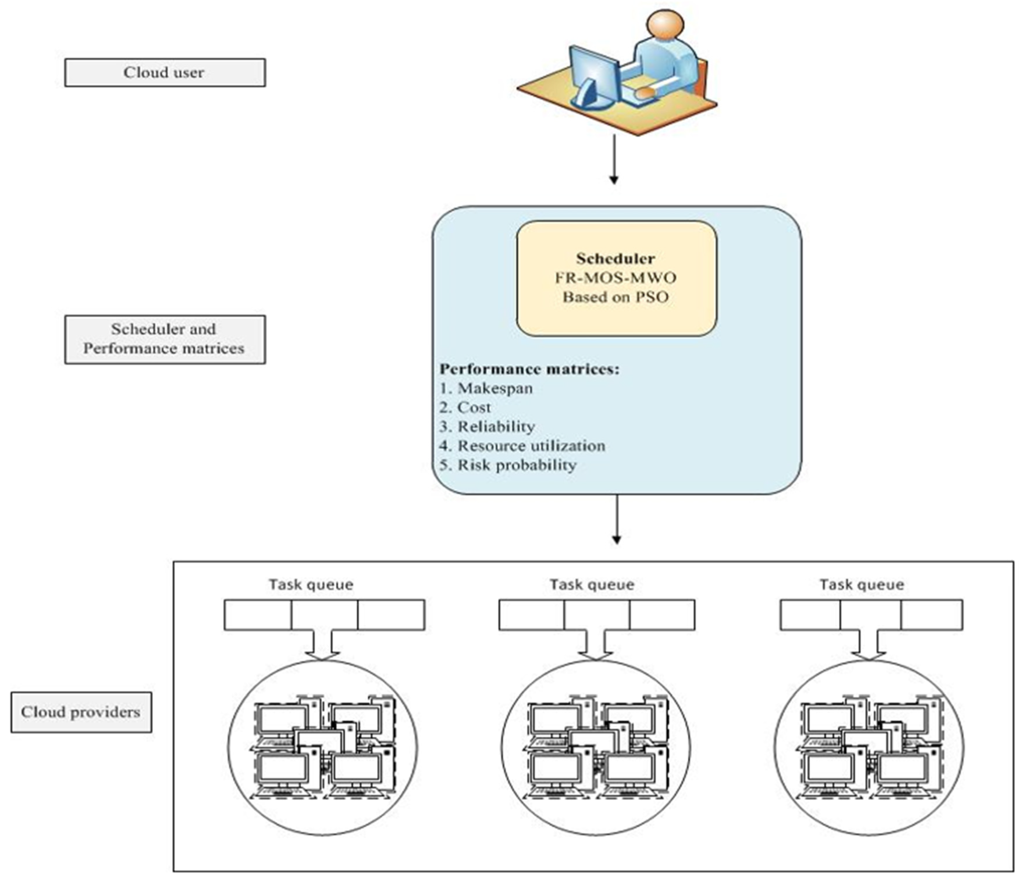
3. Scheduling Scenario

By specifically focusing on reliability, makespan, cost, workflow model, multi-cloud model, resource utilization, risk probability, and problem formulation, this section discusses the workflow scheduling model, metrics, and aspects. Five QoS requirements are taken into consideration in the proposed FR-MOS-MWO algorithm: cost, risk probability, makespan, resource utilization, and reliability. The scheduling model is shown in Figure 1, and the notations used in this study are described in Table 1 of the cited reference [34].

Designing the framework for a cloud user workflow application is part of the first phase. The distribution of workflows to a suitable cloud infrastructure should satisfy the VM types and workflow requirements. Each cloud service provider has a task queue, and tasks are carried out in accordance with the workflow hierarchy. Due to the infinite number of VM resources that cloud users have access to, simultaneous services are offered for running tasks based on dependency relationships. It is critical to understand that each cloud service provider in a multi-cloud environment has its own performance and pricing trends.

3.1. Workflow Model

To accomplish a certain goal, a workflow—a collection of scheduled activities—must be followed in any order. Workflows are collections of simple steps created to handle more complicated issues [35]. These processes must follow a consistent pattern in order to ensure coherence and increase efficiency in carrying out the desired activities. The purpose of a workflow is to specify the configuration, execution, and monitoring of several activities.

Workflow can be seen as a node-and-edge direct acyclic graph (DAG). W = (T, E) can be used to represent it, where T = {t₀, t₁,…, t_i,…, t_n−1} is the task set. The task dependencies are represented by a series of arcs E = {(t_i,t_j)|t_i,t_j $\mathsf{ϵ}$ T}. T_entry is the entry task in each workflow, and T_exit is the exit task. Furthermore, each task has a pre(t_i) and a successor set succ(t_i). Each task is carried out following the execution of its predecessor. Task t_i has an assigned weight W(t_i), which measures the workload in terms of compute units (CUs). The output data size of task t_i that needs to be transmitted to task t_j is denoted by the symbol D(t_i,t_j).

3.2. Multi-Cloud Architecture

Google Compute Engine, Amazon EC2, and Microsoft Azure are the three cloud service providers that are the focus of this study. In this section, we will examine the multi-cloud architecture, which enables users to access virtual machines (VMs) from many cloud providers with various price structures. For instance, Amazon EC2’s cost in 2018 varied depending on the service’s availability. Every incomplete clock eventually advances to full hours. Similarly, Azure subscribers in 2018 were paid per minute. After the first ten minutes of VM instance startup, Google Compute Engine prices were per minute in 2018. Reference [36] provides a comprehensive list of VM types across Tables 2 to 4.

In a multi-cloud context, various IaaS platforms can be made available for a collection of VMs, where VM(m) = {VM(m, 1),…, VM(m, k),…, VM(m, k_s)} and m = 1, 2,…, M. Let (m|m = 1, 2, and 3), where m stands for the different IaaS cloud providers (i.e., Amazon, Microsoft, and Google). The virtual machine instance that IaaS cloud provider m has specified is VM(m, k). Hourly costs are indicated by C(m, k), and CU refers to the VM CPU compute capacity. P(m, k) represents its processing power. We take for granted that the various cloud service providers can provide customers a limitless number of virtual machines. The bandwidth of cloud platform m is denoted by B_m, and the bandwidth between cloud platforms m and m′ is denoted by B_mm′.

3.3. Makespan Computation

Workflows and tasks on several IaaS platforms can be assigned and executed through a multi-cloud environment. Additionally, other VMs must wait before receiving tasks anew. This process results from VMs frequently sending their output to other VMs. The order of the tasks determines how the receiver output will be laid out. The grouping procedure of the workflow tasks within set A is described by Equation (1).

$$A=\sum _{t_j\in pre\left(t_i\right)}succ\left(t_j\right).$$

(1)

In the same manner as set A, the tasks in partial set B are completed. In the event where A = {t₁, t₃, t₄, t₂}, then B = {t₁, t₃} if t_i = t₄. In Equation (2), T_start(t_i) and T_end(t_i)are used to denote the task’s start and end times, respectively.

$$T_{start}\left(t_i\right)={max}_{t_j\in pre\left(t_i\right)}\left\{T_{end}\left(t_j\right)+T_{wait}\left(t_j, t_i\right)\right\},$$

(2)

T_wait(t_j,t_i) is the time it takes for task t_i to receive input data from task t_j. This wait time is shown as follows:

$$T_{wait}\left(t_j,t_i\right)=\sum _{t_z\in B}{T}_{trans}\left(t_j, t_z\right).$$

(3)

Observe that if t_i = t_entry, then T_start(t_i) = 0.

The transmission time has been calculated using the following equation:

$$T_{trans}\left(t_i\right)={max}_{t_j\in pre\left(t_i\right)}\left\{T_{end}\left(t_j\right)+T_{wait}\left(t_j,t_i\right)\right\}+T_{trans}\left(t_j,t_i\right),$$

(4)

where T_trans(t_j, t_i) is the transmission time between t_i and t_j.

$$T_{trans}=\left\{\begin{array}{c}D\left(t_j,t_i\right)/B_m,\\ D(t_j,t_i)/B_{mm\prime }, m\ne m\prime \end{array} \right.$$

(5)

Task t_i therefore has a receiving time provided by

$$T_{rece}\left(t_i\right)=T_{trans}\left(t_i\right)-T_{start}\left(t_i\right).$$

(6)

The size of data for each task t_i determines how long it takes to execute [30,37]. The execution time for various tasks on various VMs(m, k) can be calculated using the Equation below.

$$T_{exec}\left(t_i,VM\left(m,k\right)\right)=\frac{W\left(t_i\right)}{P\left(m,k\right)} .$$

(7)

For the completion time of each task, The VM(m,k) in CU’s processing capacity can be utilized. Therefore,

$$T_{end}\left(t_i\right)=T_{start}\left(t_i\right)+T_{rece}\left(t_i\right)+T_{exec}\left(t_i, VM\left(m,k\right)\right).$$

(8)

Then,

$$makespan=T_{end}\left(t_{exit}\right).$$

(9)

The deadline is the amount of time needed to complete the scheduling using VMs with the bare minimal processing capacity.

3.4. Cost Computation

IaaS platforms employ the multi-cloud model in their own pricing models. The time that passes between the start time and the finish time is used by the existing workflow algorithms to determine how long the VM will be rented for [30,36,37,38]. The VM terminates after the task is done, and the output is passed to the task’s successor. The priority of data transfer is impacted by the order of tasks. You can specify the sending time of task t_i as follows:

$$T_{send}\left(t_i\right)=\sum _{t_j\in succ\left(t_i\right)}{T}_{trans}(t_i, t_j).$$

(10)

Equation (11) specifies the rental time of task t_i for the VM executing on VM(m, k).

$$T_{rent}\left(t_i,VM\left(m,k\right)\right)=T_{rece}\left(t_i\right)+T_{exec}\left(t_i, VM\left(m,k\right)\right)+T_{send}\left(t_i\right).$$

(11)

Following that, the VM renting cost for task t_i on each IaaS platform is determined.

Equation (12) expresses the cost of task t_i on VM(1,k) for Amazon EC2, which charges per hour.

$$cost\left(t_i, VM\left(1,k\right)\right)=⌈T_{rent}(t_i,VM\left(1,k\right))/T_{minute}⌉ . C\left(1,k\right),$$

(12)

where T_minute = 60.

Due to Microsoft Azure’s per-minute pricing, the cost of task t_i’s execution on VM(2,k) is as shown in Equation (13).

$$cost\left(t_i, VM\left(2,K\right)\right)=T_{rent}\left(t_i,VM\left(2,k\right)\right).C(2,k)/T_{minute.}$$

(13)

After the first ten minutes, Google charges by the instance per minute. In Equation (14), these costs are shown as the task cost on VM(3,k), where T_ten = 10.

$$cost\left(t_i,VM\left(3,k\right)\right)=\left\{\begin{array}{c}{T}_{ten}.C(3,k)/T_{minute}, if T_{rent}\left(t_i,VM\left(3,K\right)\right)\le T_{ten}\\ T_{rent}\left(t_i,VM\left(3,k\right)\right).C(3,k)/T_{minute}, otherwise\end{array}\right.$$

(14)

Using Equation (15), the cost of the workflow can be determined.

$$cost=\sum _{t_i\in T}cost\left(t_i,VM\left(m,k\right)\right).$$

(15)

The highest priced VMs in the critical path can be used to identify the budget constraint when scheduling workflows.

3.5. Resource Utilization Computation

The effective allocation of resources for cloud operations depends on scheduling. In many scheduling systems, tasks are assigned to achieve a balance between cost-effectiveness, resource utilization, and makespan [39]. When compared to expensive resources, cheaper ones require more time to execute tasks, indicating that the CPU of a VM maximizes resource utilization at the expense of cost. A requested VM’s total capacity is determined by using the equation

$${VMs}_{requestedMIPS}=\sum P\left(m,k\right).$$

(16)

Each workflow’s percentage of workflow utilization can be calculated using Equation (17).

$$utilization=\frac{{VMs}_{requestedMIPS}}{{VMs}_{availableMIPS} }\times 100.$$

(17)

Because customers often expect to deal with a service provider that offers high-resource utilization, the value of max.utilization in Equation (33) is set to 100%.

3.6. Reliability Computation

Cloud computing failures are inevitable. Failures might be internal (such as software bugs, hardware problems, power issues, etc.) [40,41], or external (such as hazardous online attacks) [42,43]. Failure during task workflow can also result from short-term failures. The Poisson distribution can be used as the basis for a failure case [7,44,45]. It is calculated by finding the reliability exponent such that task t_i is successfully completed in VM(m, k):

$$rel\left(t_i\right)=\exp \left(-{\lambda }_m.T_{rent}\left(t_i,VM\left(m,k\right)\right)\right),$$

(18)

where the failure rate of the cloud service provider fulfills λm > 0 (m = 1, 2, 3).

Multi-cloud failure coefficients differ between IaaS platforms. Any issue that arises within the rental period will result in the task’s failure. The reliability of the workflow can be assessed using Equation (19), provided that the failures are independent.

$$reliability=\prod _{t_i\in T}rel\left(t_i\right).$$

(19)

If the maximum failure coefficient is specified as λ_max = max{λ_m|m = 1, 2, 3} and the minimum failure coefficient is specified as λ_min = min{λ_m|m = 1, 2, 3}, then the resulting scheduling workflow for reliability might be either maximum (rel_max) or minimal (rel_min). Additionally, based on the task scheduling procedure, various workflow results are produced in various clouds. Therefore, cloud users need to set rel_c ϵ [rel_min, rel_max] as the appropriate reliability constraint for a scientific workflow application.

3.7. Workflow Risk Probability

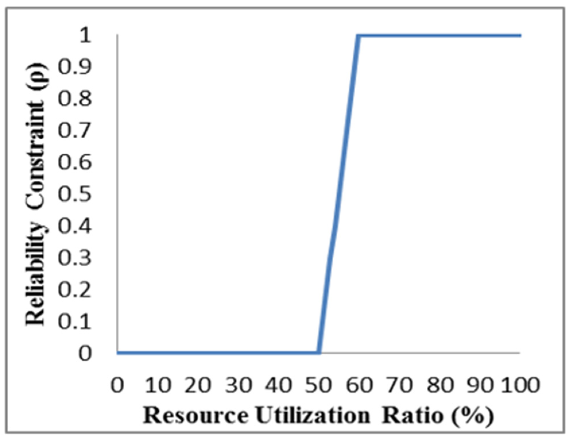
Because there are hazards to employing workflow applications in a cloud computing environment, security awareness is critical for quantitative service evaluation. During the workflow, the risk analysis model determines the risk rate [42]. The risk distribution is based on the Poisson probability distribution for each defined time, and the model assumes that the probability of risks is governed by the level of security. As shown in this section, an exponential distribution can be utilized to define the risk likelihood of the task for the last security service [46,47]

The three main cloud threats are snooping, modification, and spoofing. To safeguard scientific workflow applications, three security services—namely, authentication, integrity, and confidentiality are used [48]. Users can achieve an effective protection against different risks and attacks by dynamically integrating these security services. According to the proposed model, a typical activity will include three different types of security services with varying user-defined security rates. The collection of security requirements ${sr}_i$ for task t_i, for instance, can be expressed as a q-tuple ${sr}_i=\left[{sr}_i^1,{sr}_i^2,\dots ,{sr}_i^l,\dots ,{sr}_i^q\right],$ where ${sr}_i^l$ denotes the needed security level of the lth security service and q = 3.

$$P\left(t_i,{sl}_i^l\right)=\left\{\begin{array}{c}0, if {sr}_i^l\le {sl}_i^l\\ 1-exp\left(-{\lambda }^l\left({sr}_i^l-{sl}_i^l\right)\right), otherwise, l\in \left\{a,g,c\right\}\end{array} \right.$$

(20)

The authentication, integrity, and confidentiality services are each represented by a, g, and c, respectively.

For various cloud environments, the risk coefficient ${\lambda }^l$ varies. For instance, at the data center, 3 snooping attacks, 2.5 changes, and 1.8 spoofing attacks may be conducted in a given period of time. The negative exponent demonstrates that as the difference between ${sr}_i^l \mathrm{a}\mathrm{n}\mathrm{d} {sl}_i^l$ increases, the probability of failure rises. The risk can arise from massive network attacks or inaccessible security challenges. As a result, taking into consideration all security services, the risk probability for task t_i is as follows:

$$P\left(t_i\right)=1-\prod _{l\in \left\{a,g,c\right\}}\left(1-P\left(t_i,{sl}_i^l\right)\right).$$

(21)

The workflow risk probability P(T) with task set T can be calculated according to Equation (22).

$$P\left(T\right)=1-\prod _{t_i\in T}\left(1-P\left(t_i\right)\right).$$

(22)

This workflow risk probability will be used as a QoS constraint for problem formulation in Section 4. The algorithms for confidentiality, accessibility, and data integrity can be located in Tables 1 to 3, as outlined in reference [48,49]. Each algorithm is assigned a security rating ranging from 0.08 to 1 based on its cryptographic algorithm efficiency. Let ${sl}_i=\left[{sl}_i^1,{sl}_i^2,\dots ,{sl}_i^l,\dots ,{sl}_i^q\right]$ represent the levels of security services for task $t_i$, and ${sl}_i^l$ represent the level of the $l$th security service task $t_i$ has received.

3.8. Fuzzy Logic

In 1965, Lutfy Zadeh established the concept of fuzzy logic [50]. The principle provides a modern statistical paradigm for formalizing and evaluating collections of functions. The fuzzy logic naturally extends the common language and interprets human conduct [51].

Definition 1.

Let X be the absolute reference for an associate. Features of a typical X and its subset A, µ_A: X → {0,1} are as follows defined: ${\mu }_A\left(x\right)=\left\{\begin{array}{c}1 : x\in A\\ 0 : x\notin A \end{array}\right.$for each x $\in$ X, ${\mu }_{A\left(x\right)}$ Only one of the values from the sets 0 and 1 will be used.

Definition 2.

Each element of X is connected with a function that is assigned to a number that is within the range of [0,1] if set ${\mu }_A$is made up of two integers [0,1] that are mapped to a range between [1,0]. A is a fuzzy set as a result. If ${ \mu }_A\left(x\right)\in \left\{\mathrm{0,1}\right\}$, then set A’s membership is ambiguous. As a result, we provide a multi-objective algorithm for scheduling scientific workflows using a fuzzy approach where the reliability constraints are determined by resource utilization.

3.9. Problem Description

This study seeks to optimize resource reliability while reducing risk probability, makespan, and cost. So, WF = (T,E) is used to represent the workflow. Thus, the workflow is represented as WF = (T,E). The main objective is scheduling Γ = (Loc, Ord, R), where Loc = {loc(t₀), loc(t₁)…, loc(t_n−1)} is the task in the workflow to be executed, Ord = {ord(t₀), ord(t₁),…, ord(t_n−1)} the task’s waiting time (the task’s order must also represent dependence relations) is mostly determined by the order in which the data are transferred, and R = {R₀, R₁,…, R_i,…, R_n−1} is a group of resources that support the entire workflow with R_i = (t_i, VM(m; k), T_start(t_i), T_end(t_i)).

We then formally outline the multi-objective optimization problem.

$$\mathrm{Minimize}: F\left(\Gamma \right)=\left(makespan, cost, risk probability\right).$$

(23)

$$\mathrm{Maximize}: { F}^{\prime }\left(\Gamma \right)=\left(resource utilization, total reliability\right).$$

(24)

$$\mathrm{Subject} \mathrm{to}: reliability \ge {rel}_c .$$

(25)

Previous studies have designed task execution scheduling algorithms [30,37,42] but no priority has been given to the transmission order of the data, despite it being particularly important when developing a scheduling strategy. Therefore, we take into account the importance of data transmission.

4. Multi-Objective Optimization Methods

In this section, different approaches for obtaining the Pareto optimum set are proposed, and the effectiveness of these multi-objective optimization methods is compared. According to [36], the Pareto optimal solutions must be exact and uniformly distributed. Thus, three common efficacy metrics (distance distribution, coverage ratio, and maximum distribution ratio) are used to evaluate archive collections (Pareto front) in the suggested algorithms and additional derived algorithms.

4.1. Particle Swarm Optimization (PSO)

PSO, a computational method based on swarm intelligence and an evolutionary concept, was created by Kennedy and Eberhart in 1995 [52]. PSO, a computational method based on swarm intelligence and an evolutionary concept, was created by Kennedy and Eberhart in 1995 [52]. PSO simulates a bird’s hunting strategy. To address problems involving single-objective optimization, the PSO algorithm was initially designed. The exploration of its usage to solve a multi-objective issue solution was motivated by its superior search capabilities [53,54,55]. One of the intriguing heuristic algorithms utilized in various plans to address various issues, including cloud computing task/workflow scheduling issues, is PSO. An ideal value was discovered after generations of updates in PSO’s initial population of random solutions. Regular PSO does not use evolutionary operators like crossover and mutation, unlike some other meta-heuristic algorithms [56]. Regarding its capacity for rapid convergence, PSO has an edge over evolutionary algorithms. Furthermore, by changing some of the formulas and properties of PSO or by combining PSO with other metaheuristic algorithms, certain flaws in PSO, such as local optima, can be fixed [57]. The core element of PSO is the particle that travels through the search region. The direction and velocity of the particles determine how they move. The best historical locations are combined with random disturbances to create velocity. The velocity and position update functions are represented by Equations (26) and (27), respectively.

$${\stackrel{⃑}{v}}_i\leftarrow w.{\stackrel{⃑}{v}}_i+{\phi }_1.{rd}_1.\left({\stackrel{⃑}{p}}_i-{\stackrel{⃑}{x}}_i\right)+{\phi }_2.{rd}_2.\left({\stackrel{⃑}{g}}_i-{\stackrel{⃑}{x}}_i\right),$$

(26)

$${\stackrel{⃑}{x}}_i\leftarrow {\stackrel{⃑}{x}}_i+{\stackrel{⃑}{v}}_i,$$

(27)

If rd₁ and rd₂ ϵ [0,1] are made up values based on the random uniform distribution, w is the inertia weight and φ₁ and φ₂ are positive integers [58]. The best local position ${\stackrel{⃑}{p}}_i$, current position ${\stackrel{⃑}{x}}_i$, and velocity ${\stackrel{⃑}{v}}_i$ of each PSO particle are represented by a three-dimensional vector. A PSO algorithm-determined filter solution is indicated by position ${\stackrel{⃑}{ x}}_i$. Every time the fitness value for the current position ${\stackrel{⃑}{x}}_i$ is higher than the fitness value for the previous position, the current position is put in the vector ${\stackrel{⃑}{p}}_i$. Eventually, the communication between the particles determines the best global position ${\stackrel{⃑}{g}}_i$ for all particles [59].

4.2. Multi-Objective Pareto Optimal Approach

Multi-objective optimization issues are frequently solved using the Pareto optimality approach. This approach gives every objective the same weight and simultaneously optimizes them. the Pareto optimality principle states that solution X prevails over another solution Y if both of these conditions are true:

• In all objectives, solution X is not worse than solution Y.
• X is simply superior to Y in at least one objective.

Thus, the transition from Y to X optimizes all objectives without affecting others. The optimal or ideal Pareto reflects the best balance between objectives. These solutions (representing the Pareto frontier) are also defined as non-dominant because there is no existing alternative that improves objective achievement without hindering other objectives. The downside of this strategy is that it does not give an optimum solution, but it proffers an equally effective set of configurations. Although the final decision appears to have been taken, the relation between the optimization objectives can be analyzed without including highly inefficient configurations. This step can be achieved by identifying the optimum solution in the Pareto front [60].

Pareto Optimality Method

Harmonizing competing objectives is a key component of multi-objective optimization. This process is mathematically expressed in Equation (28).

Minimize:

$$F\left(\stackrel{⃑}{x}\right)=\left(f_1\left(\stackrel{⃑}{x}\right),f_2\left(\stackrel{⃑}{x}\right),\dots ,f_k\left(\stackrel{⃑}{x}\right)\right),$$

(28)

where k represents the number of objectives, $\stackrel{⃑}{x}\in X$ is the decision variables’ vector, and X is the decision space. Multi-objective optimization typically leads to many solutions, but researchers find the Pareto optimal solution during analysis.

For ${\stackrel{⃑}{x}}_1,{\stackrel{⃑}{x}}_2\in X,$ ${\stackrel{⃑}{x}}_1$ is considered to dominate ${\stackrel{⃑}{x}}_2$ only if

$$\forall i:f_i\left({\stackrel{⃑}{x}}_1\right)\le f_i\left({\stackrel{⃑}{x}}_2\right)˄\exists j:f_j\left({\stackrel{⃑}{x}}_1\right)<f_j\left({\stackrel{⃑}{x}}_2\right).$$

(29)

If another solution ${\stackrel{⃑}{x}}^{*}$ does not outperform it, then it meets the criteria for being a Pareto optimum solution in this study. The Pareto front set is used to display the optimal results of workflow scheduling in a multi-cloud environment within the addressed objective space. Γ* schedule dominates Γ if (a) cost, makespan, and risk probabilities (or at least one of them) are less than those in Γ, and (b) if both reliability and resource utilization (or at least one of them) are more than those in Γ. Workflow scheduling problems are NP-complete problems. As such, an approach that converges to sub-optimal solutions is considered. However, evolutionary algorithms (EAs) [30,34,53,54,61,62,63,64,65] have shown to be effective in resolving these issues.

4.3. Weighted Sum Function

Using weighted sum factors, the weighted sum function approach is used to aggregate the features of a multi-objective issue into a single feature. The weighted sum approach is more efficient and easier to use than Pareto optimality. Prior knowledge of the connections between the derived objectives, however, is essential. Furthermore, this strategy does not define how the variable affects certain design objectives.

4.3.1. Minimum Weight Optimization (MWO) Method

The proposed method can yield results indicating a variety of cost-makespan trade-offs and reliability-resource utilization relationships from which cloud clients can select. As the first stage, the weighting of each possibility is decided. If x_ij is considered to be a beneficial metric, we apply Equation (30) to normalize the values of each attribute, and if it is not, we use Equation (31). The concept of MWO revolves around selecting the optimal alternative from a pool of solutions. This is achieved by comparing the weights of all alternatives and identifying the one with the minimum weight. This process effectively narrows down the search, allowing for continuous iterations in pursuit of an increasingly superior solution.

$${\overline{x}}_{ij}=1-\frac{x_{ij}}{Max{x}_{ij}}$$

(30)

$${\overline{x}}_{ij}=\frac{x_{ij}}{Max{x}_{ij}}$$

(31)

The weighted sum model (WSM) is calculated using Equation (32) for all alternatives.

$$W=\sum _{j=1}^n{\overline{x}}_{ij}$$

(32)

The W-values indicate that the potential alternatives are weighed. Among the group members, a higher priority is given to the member with the lowest W-value. In contrast to the multi-criteria decision-making (MCDM) method, MWO does not require users or experts to assign a weight to each attribute. The makespan, cost, utilization of resources, reliability, and risk probability can all be normalized using Equation (33). We normalize the execution cost by (cost/budget), the makespan by (makespan/deadline), the resource utilization by (1—utilization/maximum utilization), the reliability by (1—reliability/maximum reliability), and the risk probability by (risk probability/maximum risk probability) for the case with different constraints. After normalization, if all values meet their individual constraints, they should not all be bigger than one. The alternate particle or schedule can then be simply determined using the optimal solution.

$$W=\frac{cost}{budget}+\frac{makespan}{deadline}+\frac{risk.prob}{max.risk.prob}+\left(1-\frac{utilization}{max.utilization}\right)+\left(1-\frac{reliability}{max.reliability}\right)$$

(33)

Let $budget$, $deadline$, $max.risk.prob$, $max.utilization$, and $max.reliability$ denote the budget, deadline, maximum risk probability, maximum utilization, and maximum reliability constraints, respectively. The constraints (cost, $espan$, $risk.prob$, $utilization$, and $reliability)$ are characterized as scheduling objectives. If and only if the workflow fits the following criteria, it is considered to be a feasible schedule:

$$\begin{gathered} cost\le budget\wedge makespan\le deadline\wedge risk.prob\le max.risk.prob\wedge utilization \\ \hspace{0.33em}\hspace{0.33em}\hspace{0.33em}\le max.utilization\wedge totalreliability\le max.reliability \end{gathered}$$

(34)

PSO multi-cloud workflow scheduling difficulties are solved by the FR-MOS algorithm. As a result, we compare our proposed method to other decision-making methods that employ multi-objective scheduling algorithms. (such as MCDM, WASPAS, and linear normalization I & II) in a multi-cloud environment. Comparatively, the MWO method outperforms other methods with respect to optimizing scheduling processes with the FR-MOS algorithm.

4.3.2. Weighted Aggregated Sum Product Assessment (WASPAS) Method

WASPAS’s primary processes are the identification of attributes and alternatives, the estimation of attribute weights, decision-making, and the selection of the final solution [5].

• Decision-Making and Selecting a Definitive Solution

The ranking of each possibility for making decisions is necessary for the WASPAS’s final steps. The normalizer function is applied to determine the rank of each alternative mapped to the values of each attribute according to Equation (35) if the maximum $x_{ij}$ is preferable or Equation (36) if otherwise.

$${\overline{x}}_{ij}=\frac{x_{ij}}{\mathit{Max}{x}_{ij}}.$$

(35)

$${\overline{x}}_{ij}=\frac{\mathit{Min}{x}_{ij}}{x_{ij}}$$

(36)

The WASPAS method combines two famous MCDM approaches. The first optimal criterion (i.e., Equation (37)) calculates the weighted sum model (WSM) of all alternatives, while the other (Equation (38)) is a WPM (weighted product model).

$$Q^1=\sum _{j=1}^n{\overline{x}}_{ij}\times w_j$$

(37)

$$Q^2=\prod _{j=1}^n{\left({\overline{x}}_{ij}\right)}^{w_j}$$

(38)

where w_j is the weight of the jth attribute. The degree of importance of the attributes determined by w_j is defined by the user. Equation (39) constitutes the final step used in WASPAS.

$$Q_i=0.5Q^1+0.5Q^2$$

(39)

Now that the candidate options have been ranked by Q-values, the group member with the greatest Q-value is given top priority.

4.3.3. Multi-Criteria Decision-Making (MCDM) Method

A strategy for multi-objective problems is the multi-criteria decision-making approach. It has been developed and applied widely to resolve complex decision-making problems [66]. Many approaches and theories to solve decision-making problems with multiple criteria have been developed over the years [67]. Through an analysis of numerous criteria, MCDM approaches can assist in identifying the best among a number of possibilities. This identification is accomplished by weighing the advantages and disadvantages of various adaption possibilities [68]. There are many MCDM methods, such as COPRAS, WSM, TOPSIS, AHP, and VIKOR. In our study, we use WSM because it is more stable when compared to COPRAS [69] and is an intuitive decision-making process; The calculating process is very simple, this approach combines the weights and values of the variables into a single magnitude. Normalized evaluation values help in visually calculating the differences between alternatives. This approach is ideal for evaluating one alternative [70]. According to Chakravarthi et al. (2020), when combined with other criteria, TOPSIS is particularly tough to weigh and preserves consistency of judgment. Furthermore, Euclidean distance implementation does not consider attribute correlation [71].

The normalizer function will be used to transform the value of each attribute in the initial step of determining the rank of each alternative according to Equation (35) if $x_{ij}$ is a required metric or Equation (36) if otherwise. For all alternatives, MCDM uses WSM, as expressed in Equation (40).

$$W=\sum _{j=1}^n{\overline{x}}_{ij}\times w_j$$

(40)

where $w_j$ is the weight of the jth attribute.

This characteristic is one of the cons of MCDM. In our experiment, we use an equal weight for all attributes. The alternative candidates are classified according to the W-values, and among the group members, the individual with the highest W-value is given a higher priority.

4.3.4. Linear Normalization

We apply the normalizer to each attribute in linear normalization in accordance with Equation (35) if $x_{ij}$ is beneficial or Equation (41) if it is not.

$${\overline{x}}_{ij}=1-\frac{x_{ij}}{\mathit{Max}{x}_{ij}}$$

(41)

The normalizer function and WSM (Equation (42)) are applied to each alternative.

$$W=\sum _{j=1}^n{\overline{x}}_{ij}$$

(42)

The W-values are used to rank the candidate alternatives, and the group member with the greatest W-value is given priority over the others. This study adopts linear normalization II. We use Equation (43) instead of Equation (41), and the difference between their results is detailed in the Results section.

$${\overline{x}}_{ij}=\frac{\mathit{Min}{x}_{ij}}{x_{ij}}$$

(43)

5. The Proposed Algorithms

In this article, we propose two PSO-based methods for scheduling optimization with multi-attribute consideration. The first algorithm combines our previous FR-MOS algorithm with a novel method of decision-making called MWO to produce a superior collection of Pareto front solutions. The second algorithm creates a multi-objective Pareto optimization by combining the FR-MOS algorithm and the Pareto optimization method.

5.1. The Five-Objective Case Study

We explore a situation with five crucial real-life objectives: cost, makespan, resource utilization, reliability, and risk probability. The resource provider is concerned with resource utilization and risk probability, whereas the users are concerned with the remaining objectives. Regarding numerous crucial classification criteria, these objectives are different [72,73], as summarized in

Table 1. Classification of objective functions.

Objective	Aggregation	Direction
Makespan	Additive	Min
Cost	Additive	Min
Resource Utilization	Additive	Max
Reliability	Multiplicative	Max
Risk Probability	Multiplicative	Min

.

5.2. Determining Attributes and Alternatives

The following decision matrix is used to start any decision-making problem with various criteria:

$$\mathrm{A}=\left[\begin{array}{cccc}{\mathrm{x}}_{11}& {\mathrm{x}}_{12}& \dots & {\mathrm{x}}_{1\mathrm{n}}\\ {\mathrm{x}}_{21}& {\mathrm{x}}_{22}& \dots & {\mathrm{x}}_{2\mathrm{n}}\\ {\mathrm{x}}_{31}& {\mathrm{x}}_{32}& \dots & {\mathrm{x}}_{3\mathrm{n}}\\ {\mathrm{x}}_{\mathrm{m}1}& {\mathrm{x}}_{\mathrm{m}2}& \dots & {\mathrm{x}}_{\mathrm{m}\mathrm{n}}\end{array}\right],$$

where n is the number of attributes that should be optimized and m is the number of candidate alternatives (in this study, the members of the Pareto front set) from which one should be chosen (for example, in our case, we have five objectives: cost, makespan, risk probability, reliability, and utilization).

5.3. FR-MOS-MWO Algorithm

For multi-cloud applications, a PSO-based FR-MOS-MWO algorithm has been proposed (detailed in Algorithm 1). The initialization process begins with initializing the PSO and scheduling parameters (lines 1–6). The output parameter evaluation occurs during workflow scheduling (lines 17–28). In order to choose the feasible solution, there are then two reliability restrictions [62]. According to the following description, (1) the best solution (lines 31–34) is one of the alternatives and (2) the most suitable selection with the lowest reliability constraint shall be selected if all possible solutions are not feasible [74]. Therefore, only solutions that are feasible (lines 38–43) are saved. In order to identify several optimal solutions for multi-objective issues, the method that is selected is utilized to assess the optimal location (line 46). The algorithm continues to execute until the final criteria is fulfilled (line 7).

Algorithm 1: FR-MOS-MWO

$\mathit{B}\mathit{E}\mathit{G}\mathit{I}\mathit{N}$ 1: $Set the number of particles Np;$ 2: $Set A=\varnothing ;/$/$initially empty archive, record non-dominated solution$ 3: ${initialize \{ {\stackrel{⃑}{v}}_{i }, {\overrightarrow{x}}_i ,{\overrightarrow{p}}_i , {\overrightarrow{g}}_i \} }_{i=1}^N ; /$/$random location and velocity$ 4: $initialize \{reliability=makespan=cost=utilization=0\};$ 5: ${Set \{{\overrightarrow{p}}_i={\overrightarrow{x}}_i, {\overrightarrow{g}}_i=, {\overrightarrow{x}}_i \}}_{i=1}^N ;$  6: $calculate{ \left\{p_i, g_i\right\}}_{i=1}^N;$  7: $\mathit{W}\mathit{h}\mathit{i}\mathit{l}\mathit{e} \mathit{idx}<N_{IT }$//$N_{IT} is the number of iteration time$ 8: $\mathit{f}\mathit{o}\mathit{r} each particle i to N_P$ 9: ${\overrightarrow{v}}_i\leftarrow w.{\overrightarrow{v}}_i+{\phi }_1. {rd}_{1 }.\left({\overrightarrow{p}}_i-{\overrightarrow{x}}_i\right)+{\phi }_2.{rd}_2.\left({\overrightarrow{g}}_i-{\overrightarrow{x}}_i\right);$//$update velocity$ 10: ${\overrightarrow{x}}_i \leftarrow {\overrightarrow{x}}_i+{\overrightarrow{v}}_i;$ //update position 11: $\mathit{f}\mathit{o}\mathit{r} task t_i in Ord$ //$traverse tasks in order$ 12: $\mathit{if} t_i=t_0$ //$entry task$ 13: $Set T_{start}\left(t_i\right)=0;$ //$this is also the start time of workflow$ 14: $\mathit{e}\mathit{l}\mathit{s}\mathit{e}$ 15: $Set T_{start}\left(t_i\right) according to Equation \left(2\right);$ 16: end if 17: $Compute T_{rece}\left(t_i\right) based on Equation \left(6\right);$ 18: $Compute T_{exec}\left(t_i\right) based on Equation \left(7\right);$  19: $Compute T_{end}\left(t_i\right) based on Equation \left(8\right);$ 20: $Compute Task risk probability P\left(t_i\right)based on Equation \left(21\right)$ 21: $Compute the rel\left(t_i\right) based on Equation \left(18\right);$ 22: end for 23: $Calculate makespan according to Equation \left(9\right);$ 24: $Calculate cost according to Equation \left(15\right);$ 25: $Calculate resource utilization according to Equation \left(17\right);$ 26: $Calculate workflow risk probability according to Equation \left(22 \right);$ 27: $Set reliability coefficient \rho according to Equation \left(47\right);$ 28: $Calculate reliability according to Equation \left(19\right);$ 29: $Calculate workflow weight according to Equation \left(33\right);$ 30: $Define \theta \left({\overrightarrow{x}}_i\right)=max( 0 , {rel}_c-reliability$) 31: If $\theta \left({\overrightarrow{x}}_i\right)==0 \wedge \theta \left({\overrightarrow{p}}_i\right)==0$ //${\overrightarrow{x}}_i and {\overrightarrow{p}}_i are all feasible solutions$ 32: If $W_{{\overrightarrow{x}}_i}<W_{{\overrightarrow{p}}_i}$//$update personal {\overrightarrow{p}}_i$ 33: $Set {\overrightarrow{p}}_i={\overrightarrow{x}}_i;$ 34: end if 35: else 36: $Set {\overrightarrow{p}}_i={\overrightarrow{x}}^{\prime }=argmin\left\{\theta \left({\overrightarrow{x}}_i\right), \theta \left({\overrightarrow{p}}_i\right)\right\};$ 37: end if 38: If $\theta \left({\overrightarrow{x}}_i\right)==0$ //$only the feasible solution will be added to A$ 39: for $\forall \overrightarrow{x}\in A \wedge W_{{\overrightarrow{x}}_i}<W_{\overrightarrow{x}} /$/update A 40: $A=\{ \overrightarrow{x}\in A| W_{\overrightarrow{x}}{>W}_{{\overrightarrow{x}}_i}\};$ //$remove points from A$ 41: $A=A\cup {\overrightarrow{x}}_i;$ //$add {\overrightarrow{x}}_i to A$ 42: end for 43: end if 44: $\hspace{1em}\hspace{1em}\hspace{1em}idx++$ 45: end for 46: $\hspace{1em}\hspace{1em} Randomly select global optimal position {\overrightarrow{g}}_i;$ 47: end while $\mathit{E}\mathit{N}\mathit{D}$

The fitness of each particle is estimated via the FR-MOS-MWO scheduling algorithm. The particle location Γ_c is converted into the workflow Γ by this estimation. The makespan for each task must be determined using the start time (lines 12–16). Following that, the calculation of the data receiving time T_rece(t_i), task execution time T_exec(t_i), and end time T_end(t_i) is done (lines 17–19). The task’s reliability and risk probability are then determined (lines 20–21). Finally, the cost, reliability, utilization of resources, risk probability, and makespan of workflow scheduling are determined (lines 23–28) [34].

5.4. FR-MOS-PARETO Algorithm

PSO is also used in the proposed FR-MOS-PARETO algorithm (detailed in Algorithm 2) for a multi-cloud scenario. First, the scheduling and PSO settings are initialized (lines 1–6). The performance characteristics are then evaluated as part of the workflow scheduling procedure (lines 17–28). For selecting a feasible solution, two reliability restrictions are considered [62]: (a) The most suitable solution is chosen from a set of feasible alternatives (lines 30–33). (b) Unless all alternatives are feasible, the best solution with the lowest violations of the restriction is chosen [40]. Only feasible solutions (lines 37–42) are saved. (Line 45) describes how the selection approach is utilized to determine the best position for an optimal multi-objective problem solution. (Line 7) indicates that the algorithm will continue until the final condition is met.

Algorithm 2: FR-MOS-PARETO

$\mathbf{B}\mathbf{E}\mathbf{G}\mathbf{I}\mathbf{N}$ 1: $Set the number of particles Np;$ 2: $Set A=\varnothing ;$ //$initially empty archive, record non-dominated solution$ 3: ${initialize \{ {\stackrel{⃑}{v}}_{i }, {\overrightarrow{x}}_i ,{\overrightarrow{p}}_i , {\overrightarrow{g}}_i \} }_{i=1}^N ; /$/$random location and velocity$ 4: $initialize \{reliability=makespan=cost=utilization=0\};$ 5: ${Set \{{\overrightarrow{p}}_i={\overrightarrow{x}}_i, {\overrightarrow{g}}_i=, {\overrightarrow{x}}_i \}}_{i=1}^N ;$  6: $calculate{ \left\{p_i, g_i\right\}}_{i=1}^N;$  7: $\mathit{W}\mathit{h}\mathit{i}\mathit{l}\mathit{e} \mathit{idx}<N_{IT }$//$N_{IT} is the number of iteration time$ 8: $\mathit{f}\mathit{o}\mathit{r} each particle i to N_P$ 9: ${\overrightarrow{v}}_i\leftarrow w.{\overrightarrow{v}}_i+{\phi }_1. {rd}_{1 }.\left({\overrightarrow{p}}_i-{\overrightarrow{x}}_i\right)+{\phi }_2.{rd}_2.\left({\overrightarrow{g}}_i-{\overrightarrow{x}}_i\right);$//$update velocity$ 10: ${\overrightarrow{x}}_i \leftarrow {\overrightarrow{x}}_i+{\overrightarrow{v}}_i;$ //update position 11: $\mathit{f}\mathit{o}\mathit{r} task t_i in Ord$ //$traverse tasks in order$ 12: $\mathit{if} t_i=t_0$ //$entry task$ 13: $Set T_{start}\left(t_i\right)=0;$ //$this is also the start time of workflow$ 14: $\mathit{e}\mathit{l}\mathit{s}\mathit{e}$ 15: $\mathrm{S}et T_{start}\left(t_i\right) according to Equation \left(2\right);$ 16: end if 17: $Compute T_{rece}\left(t_i\right) based on Equation \left(6\right);$ 18: $Compute T_{exec}\left(t_i\right) based on Equation \left(7\right);$  19: $Compute T_{end}\left(t_i\right) based on Equation \left(8\right);$ 20: $Compute Task risk probability P\left(t_i\right) based on Equation \left(21\right)$ 21: $Compute the rel\left(t_i\right) based on Equation \left(18\right);$ 22: end for 23: $Calculate makespan according to Equation \left(9\right);$ 24: $Calculate cost according to Equation \left(15\right);$ 25: $Calculate resource utilization according to Equation \left(17\right);$ 26: $Calculate workflow risk probability according to Equation \left(22 \right);$ 27: $Set reliability coefficient \rho according to Equation \left(47\right);$ 28: $Calculate reliability according to Equation \left(19\right);$ 29: $Define \theta \left({\overrightarrow{x}}_i\right)=max(0 , {rel}_c-reliability$) 30: If $\theta \left({\overrightarrow{x}}_i\right)==0 \wedge \theta \left({\overrightarrow{p}}_i\right)==0$ //${\overrightarrow{x}}_i and {\overrightarrow{p}}_i are all feasible solutions$ 31: If ${\overrightarrow{x}}_i\preccurlyeq {\overrightarrow{p}}_i \vee ({\overrightarrow{x}}_i\nprec {\overrightarrow{p}}_i \wedge {\overrightarrow{p}}_i \nprec {\overrightarrow{x}}_i)$ //$update personal {\overrightarrow{p}}_i$ 32: $Set {\overrightarrow{p}}_i={\overrightarrow{x}}_i;$ 33: end if 34: else   35: $Set {\overrightarrow{p}}_i={\overrightarrow{x}}^{\prime }=argmin\left\{\theta \left({\overrightarrow{x}}_i\right), \theta \left({\overrightarrow{p}}_i\right)\right\};$ 36: end if 37: If $\theta \left({\overrightarrow{x}}_i\right)==0$ //$only the feasible solution will be added to A$ 38: for $\forall \overrightarrow{x}\in A \wedge {\overrightarrow{x}}_i\nprec \overrightarrow{x} /$/update A 39: $A=\{ \overrightarrow{x}\in A| \overrightarrow{x}\nprec {\overrightarrow{x}}_i\};$ //$remove points dominated by {\overrightarrow{x}}_i$ 40: $A=A\cup {\overrightarrow{x}}_i;$ //$add {\overrightarrow{x}}_i to A$ 41: end for 42: end if 43: $\hspace{1em}\hspace{1em}idx++$ 44: end for 45: $\hspace{1em}\hspace{1em}Randomly select global optimal position {\overrightarrow{g}}_i;$ 46: end while $\mathbf{E}\mathbf{N}\mathbf{D}$

5.5. Coding Strategy

In Equation (44), the coding strategy is shown. The multi-objective scheduling problem is resolved by deciding the order of each task and allocating each task to the location that will transmit data most effectively. The three IaaS platforms taken into consideration in this study are listed in Table 5 in [36] along with their respective search spaces for various VM types.

$${\Gamma }_c=\left(loc\left(t_0\right), loc\left(t_1\right), \dots ,loc\left(t_{n-1}\right), ord\left(t_0\right), ord\left(t_1\right), \dots ,ord\left(t_{n-1}\right)\right).$$

(44)

The number of parameters in Γ_c in Equation (44) illustrates the particle’s dimension, i.e., Ω = 2⋅n. The 0 to n − 1 positions specify the types of VMs assigned to the tasks. For each task, loc(t_i) considers the VM type and the execution location. The waiting time of tasks is affected by the order of tasks ord(t_i). Figure 2 depicts the workflow encoding plan.

Since task t₁ must be completed before task t₂ if it comes before task t₂ in the string Ord, Algorithm 3 determines the tasks’ order based on their dependencies. The scheduled tasks are first initialized, i.e., $\alpha$= {t₀} (line 2). Two groups of scheduled tasks are designated as $\gamma$ and β in line 3. The flag (line 4) captures the position of the search area, and waiting tasks are configured to be empty. Line 5 uses $space=\left[\mathrm{0,0}\right]$ to denote an unaltered entering task location. In lines 11 through 15, the Euclidean distance is utilized, and in line 16 the ideal answer is chosen from the search space. Finally, the tasks are evaluated and assigned to the schedulable set α (lines 20–24). To guarantee a more constrained search space for each task in the current schedulable task α, the search space is updated sequentially (line 26). Our suggested method provides a better trade-off than FR-MOS-PARETO, which is viewed as an innovative approach to adopting the PSO coding strategy for workflow management. To provide nearly optimum multi-objective solutions, Algorithms 1 and 3 are integrated.

Algorithm 3: Order tasks

$\mathbf{B}\mathbf{E}\mathbf{G}\mathbf{I}\mathbf{N}$ 1. Initialize 2. $\alpha =\left\{t_i\right\};$ //$schedulable entry task t_0$ 3. $\gamma =\beta =\varnothing ;$ //$the set of scheduled tasks and temporary tasks$ 4. $flag=0;$ //$record location in search space$ 5. $space=\left[\mathrm{0,0}\right]$ //$search space$ 6. end Initialize 7. $\mathit{w}\mathit{h}\mathit{i}\mathit{l}\mathit{e} \alpha \ne \varnothing$ 8. $flag=flag+\left|\alpha \right|;$ 9. $\mathit{f}\mathit{o}\mathit{r} t_{i }in \alpha$ 10. $Put all successors of task t_i into \beta ;$ 11. ${\overrightarrow{v}}_i\leftarrow w.{\overrightarrow{v}}_i+{\phi }_1. {rd}_{1 }.\left({\overrightarrow{p}}_i-{\overrightarrow{x}}_i\right)+{\phi }_2.{rd}_2.\left({\overrightarrow{g}}_i-{\overrightarrow{x}}_i\right);$ 12. ${\overrightarrow{x}}_i \leftarrow {\overrightarrow{x}}_i+{\overrightarrow{v}}_i;$  13. $\mathit{i}\mathit{f} x_{i }\notin space$ 14. $x_i=(x_i^{\prime }:min(\left|x_i^{\prime }-x_i\right|,x_i space)$ 15. $\mathit{e}\mathit{n}\mathit{d} \mathit{i}\mathit{f}$ 16. $space=space-\left\{x_i\right\};$ 17. $\gamma =\gamma +\left\{t_i\right\};$ //$add task to the set of scheduled tasks$ 18. $\alpha =\alpha -\left\{t_i\right\};$//$remove task from \alpha$ 19. $\mathit{e}\mathit{n}\mathit{d} \mathit{f}\mathit{o}\mathit{r}$ 20. $\mathit{f}\mathit{o}\mathit{r} t_{i }in\beta$ 21. $\mathit{i}\mathit{f} pre\left(t_{i }\right)\in \gamma$ 22. $\alpha =\alpha +\left\{t_i\right\};$ //$add new task to \alpha$ 23. $\mathit{e}\mathit{n}\mathit{d} \mathit{i}\mathit{f}$ 24. $\mathit{e}\mathit{n}\mathit{d} \mathit{f}\mathit{o}\mathit{r}$ 25. $Clear \beta ;$ 26. $space=\left[flag, flag+\left|\alpha \right|-1\right];$ //$update the search space$ 27. $\mathit{e}\mathit{n}\mathit{d} \mathit{w}\mathit{h}\mathit{i}\mathit{l}\mathit{e}$ $\mathbf{E}\mathbf{N}\mathbf{D}$

6. Experimental Setup and Simulation Results

The structures of the scientific workflows are shown in Figure 3. A 16 GB RAM processor with an i7 6-core was used for the experiments. SIPHT, Montage, LIGO, and CyberShake are four real-world scientific workflows that were used in WorkflowSim 1.0 to apply the suggested methodology. With [1,32] compute units, a uniform distribution was used to generate random values for rd₁ and rd₂. The cloud failure coefficients for Amazon EC2, Google Compute Engine, and Microsoft Azure were λ1 = 0.001, λ2 = 0.003, and λ3 = 0.002, respectively. The bandwidth was set to 0.1 G/s if the VMs were in the same cloud and to 0.05 G/s if they were in different clouds. In the multi-objective problem, the reliability of the workflow should be equal to or greater than the reliability constraint, according to Equation (25). For determining the highest reliability, Equation (19) was employed.

$$\prod _{i=1}^n{rel}^{max}\left(t_i\right)={rel}^{max}.$$

(45)

Particle number N_P = 50, w = 0.5, and φ₁ = φ₂ = 2.05 in FR-MOS-MWO. The FR-MOS-MWO method had 10 repeat programming, N_IT = 1000 repeat times, and N_S = 15 compensation solutions. We measured the minimal workflow reliability (rel^min) in addition to the maximum workflow reliability to ensure adequate reliability. The workflow’s reliability can be set by users as follows:

$${rel}_c={rel}^{min}+\rho .\left({rel}^{max}-{rel}^{min}\right)$$

(46)

where ρ ϵ [0,1].

In our proposed algorithm, Equation (47) shows the reliability constraint coefficient obtained after the result of the resource utilization is done via fuzzy logic [36,75].

$$\rho =\left\{\begin{array}{c}0 if\left(utilization\le 50\right) \\ \frac{utilization-50}{10}if\left(utilization>50 \&\& utilization<60\right)\\ 1 otherwise \end{array}\right.$$

(47)

The reliability constraints have to be within the proper range [rel^min, rel^max] according to Equation (46). We discovered that the non-consistency between 50 and 60 gave a better makespan-cost trade-off than MOS when we evaluated the performance of the FR-MOS-MWO method for workflow scheduling. The relationship between utilization of resources and the reliability constraint (ρ) coefficient is shown in Figure 4.

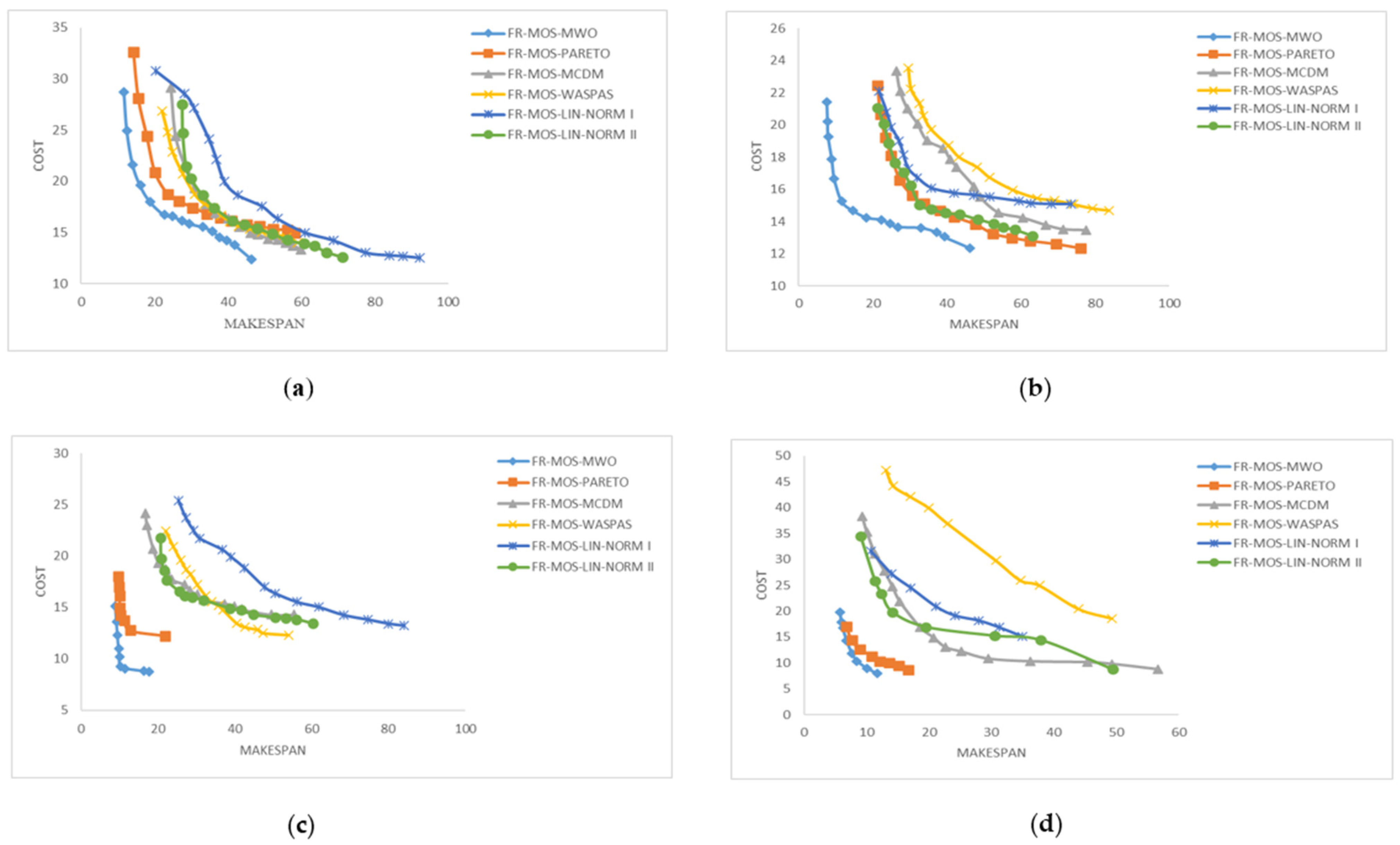
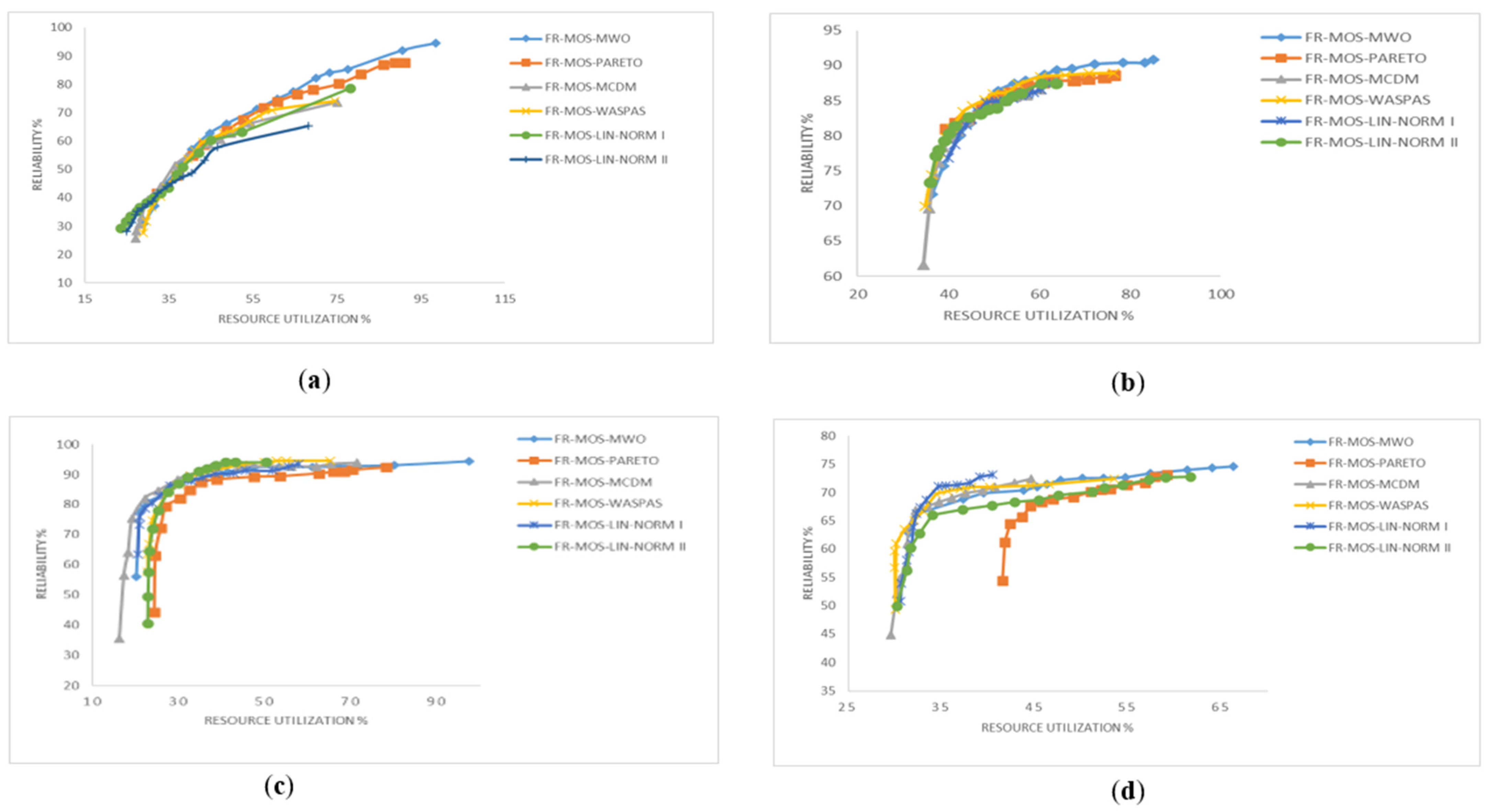
6.1. Simulation Results

The findings of the experiments are described in this section. Figure 5 displays the outcomes of various decision-making techniques used to optimize the FR-MOS algorithm for various scientific workflows. Results from the Montage workflow (Figure 5a) demonstrate that when compared to the other approaches, the FR-MOS-MWO algorithm produced the best makespan-cost trade-off. Additionally, Figure 5b demonstrates that for the makespan-cost trade-off on LIGO, FR-MOS-MWO generated the best set of alternatives. Figure 5c’s comparison of the various approaches used on CyberShake reveals that FR-MOS-MWO created solutions with the best makespan-cost trade-off. The FR-MOS-PARETO algorithm generated the second-best outcomes. The SIPHT workflow’s graphs (Figure 5d), which show similar results, can also be observed. Deductively, FR-MOS-MWO and FR-MOS-PARETO outperformed the other methods that applied the Pareto front.

The relation between resource utilization and reliability is depicted in Figure 6. The FR-MOS algorithm was employed with a variety of decision-making techniques in diverse scientific workflows. Similar to Figure 5, the results demonstrate that when compared to the other approaches, the FR-MOS-MWO achieved the best performance (i.e., high resource utilization and reliability). These outcomes show how effective our new method for decision-making is. The reliability of the workflow is determined as the product of the exponentially distributed task reliabilities, which leads to a smaller workflow reliability, according to Equation (19). For this reason, the workflow dependability was represented by the mean reliability of each workflow.

Table 2. The scheduling results of different objectives.

Workflow	Methods	Makespan (H)	Cost ($)	Resource Utilization %	Reliability %	Risk Probability %
Montage	MWO	20.10096	18.16248	98.41	94.39949675	0
	MCDM	25.28155	19.07311	74.958	73.40873522	3.68121 × 10−18
	NORMALIZATION1	24.53447	17.74348	77.902	78.49092802	1.2674 × 10−128
	NORMALIZATION2	28.57465	20.19869	67.804	64.99937426	3.67288 × 10−48
	WASPAS	36.61334	18.17652	74.189	73.70053177	6.27629 × 10−60
	PARETO	27.20506	18.12757	89.439	86.92925785	0
CyberShake	MWO	13.41054064	18.15663683	97.50642857	94.0787519	0
	MCDM	42.10671	20.40252	71.40428571	94.3438238	0.005376047
	NORMALIZATION1	25.03879	25.24809	57.87071429	93.0850308	0
	NORMALIZATION2	20.89159132	18.427447	50.08142857	90.5211898	3.3656 × 10−229
	WASPAS	45.4625	19.15031	64.28714286	95.869359	0.117599759
	PARETO	22.14941565	20.74585587	77.915	93.7694293	2.4616 × 10−167
LIGO	MWO	18.62719	19.31839	88.51	90.98273739	0
	MCDM	34.33421	22.35154	79.558	83.59184932	4.21224 × 10−79
	NORMALIZATION1	51.65373	21.31771	56.254	85.39737027	0
	NORMALIZATION2	70.20769	14.59921	63.872	87.23663633	8.716 × 10−238
	WASPAS	33.1888	21.82187	68.448	86.43662257	1.72212 × 10−11
	PARETO	45.40331	25.88293	79.322	86.90678744	0
SIPHT	MWO	5.602056079	6.79905612	66.675	73.9875787	0
	MCDM	11.24748374	11.45402866	44.59333333	71.3080864	0.471667852
	NORMALIZATION1	19.30668	36.79846	40.76166667	73.4901905	8.3689 × 10−130
	NORMALIZATION2	16.32143348	11.75497218	61.68916667	71.3719201	6.6051 × 10−126
	WASPAS	30.47000992	12.64217567	52.97416667	71.7378019	6.4918 × 10−240
	PARETO	16.05690635	13.80430791	58.17333333	73.5531058	7.61767 × 10−46

displays the outcomes of the various decision-making techniques examined in this article. In light of the competing attributes (makespan, cost, risk probability, reliability, and resource utilization), the table demonstrates that when using the Montage workflow, FR-MOS-MWO produced the best results in terms of makespan, resource utilization, and reliability; however, it had the same risk probability and high cost as FR-MOS-PARETO. FR-MOS-MWO outperformed the other algorithms for the remaining three workflows (CyberShake, LIGO, and Sipht) across all attributes. When compared to the other FR-MOS-based algorithms investigated, FR-MOS-MWO produced the best result.

6.2. Performance Measurement

Considering just one of the efficiency aspects is unlikely to be sufficient to test multi-purpose solutions, three metrics were used: Q-metric, S-metric, and FS-metric. Using these metrics is important when evaluating the Pareto front quality produced by various algorithms [54]. To assess the level of convergence of multi-objective algorithms A and B, Q-metric can be used [76,77], as stated in Equation (48).

$$Q\left(A,B\right)=\left|\Psi \right|/\left|Y\right|.$$

(48)

Y is the set of SA ∪ SB, and Ψ = Υ ∩ SA. SA and SB denote the two sets of Pareto optimal solutions for the two multi-objective algorithms A and B. Only when Q(A, B) > Q(B, A) or Q(A, B) > 0.5 is Algorithm A superior to Algorithm B. The FS measure determines the Pareto front space size. It is calculated using Equation (49) [78].

$$FS=\sqrt{\sum _{i=1}^m\underset{(x_0,x_1)\in \mathit{SA}\times \mathit{SA}}{\min }{(f_i\left(x_0\right)-f_i\left(x_1\right))}^2, }$$

(49)

Because f_i(x₀) and f_i(x₁) are two different values of the same objective function, ahigher FS value indicates greater diversity in the Pareto front. To determine the amount of uniformity of solutions, we use the S-metric as calculated in Equation (50) [36].

$$s=\sqrt{\sum _{i=1}^{N_P}{(d_i^{\prime }-\overline{d^{\prime }})}^2/N_P},$$

(50)

where N_P is the number of Pareto solutions and $d_i^{\prime }$ is the distance between the Pareto front set members.

$$\overline{d^{\prime }}=(\sum _{i=1}^{N_P}{d}_i^{\prime })/N_P.$$

(51)

While a larger value is preferable for the FS-metric and Q-metric, a smaller S-metric indicates that the algorithm has discovered a uniform solution.

For all FR-MOS-based algorithms, the relation between reliability, resource usage, and makespan-cost trade-offs is depicted in Figure 5 and Figure 6. Notably, when compared to other FR-MOS-based algorithms, the FR-MOS-MWO algorithm produced the best results for all objectives taken into account.

Table 3. Multi-objective performance metrics.

Workflow	Q-Metric	FR-MOS-MWO	FR-MOS-PARETO	FR-MOS-MCDM	FR-MOS-WASPAS	FR-MOS-LIN-NORM I	FR-MOS-LIN-NORM II
Montage	FR-MOS-MWO	-	True	True	True	True	True
	FS-metric	1.38	0.3	0.4	0.6	0.2	0.5
	S-metric	0.08	0.23	0.17	0.074	0.26	0.13
LIGO	FR-MOS-MWO	-	True	True	True	True	True
	FS-metric	0.69	0.26	0.064	0.127	0.003	0.38
	S-metric	0.022	0.107	0.153	0.119	0.121	0.038
SIPHT	FR-MOS-MWO	-	True	True	True	True	True
	FS-metric	1.01	0.839	1.0	1.84	1.72	2.59
	S-metric	0.07	0.16	0.24	0.32	0.11	0.84
CyberShake	FR-MOS-MWO	-	True	True	True	True	True
	FS-metric	0.244	0.063	0.0001	0.2	0.19	0.385
	S-metric	0.073	0.214	0.170	0.22	0.16	0.084

provides an illustration of the multi-objective performance metrics shown in Figure 5 and Figure 6. The performance of FR-MOS-MWO is superior to other FR-MOS-based algorithms if the Q-metric is set to true. Table 3 demonstrates that for all scientific workflows, the value of the Q-metric was true Q (FR-MOS-MWO, FR-MOS-based). This result demonstrates that FR-MOS-MWO’s solutions are superior to those of the other algorithms, proving that this algorithm offers the best multi-objective convergence outcome. In terms of the Montage workflow, the FS-metric value for FR-MOS-MWO was 1.38, which was higher than those of other algorithms, showing that FR-MOS-MWO produces a better level of diversity in comparison to those other algorithms. It can be shown that FR-MOS-MWO provides more uniformity in the Pareto front than other FR-MOS-based algorithms because its S-metric, which was 0.08, was less than those of the other algorithms. Regarding the LIGO workflow, FR-MOS-MWO’s FS-metric was 0.69, greater than that of the other algorithms, showing that it is more diverse than the other algorithms. The uniformity in the Pareto front of FR-MOS-MWO is better than that of the other algorithms, as evidenced by the S-metric of the algorithm being smaller for FR-MOS-MWO (0.022) than for the other algorithms. Table 3 demonstrates that using FR-MOS-MWO on SIPHT resulted in a better FS-metric value of 1.01 than FR-MOS-PARETO and FR-MOS-MCDM. FR-MOS-LIN-NORM II, in contrast, generated an FS-metric value of 2.59, showing that it offers a greater diversity than the other FR-MOS-based algorithms. The best uniformity was achieved by FR-MOS-MWO, as evidenced by the algorithm’s S-metric of 0.07, which was lower than that of the other algorithms.

FR-MOS-MWO’s FS-metric was 0.244, which was better than all other FR-MOS-based algorithms when compared to FR-MOS-LIN-NORM II’s FS-metric of 0.385, according to the CyberShake results. This result implies that FR-MOS-LIN-NORM II produced a better diversity compared to all other algorithms. FR-MOS-MWO’s S-metric value was 0.073, which was lower than that of other algorithms. As a result, when compared to other algorithms, FR-MOS-MWO generates the best uniformity. Our investigation showed that, in some instances, (MCDM) strategies outperformed the WASPAS strategy in terms of results. For instance, different MCDM techniques showed more efficacy than WASPAS in the context of the SIPHT workflow. Notably, our proposed method, MWO, consistently delivered the best results. This success can be attributed to its approach of narrowing down the research process through the use of the minimum weight criterion. Additionally, some other MCDM methods produced multiple equivalent results, which can complicate the selection of the optimum solution or leave the choice up to users, as seen with the Pareto method in prior research. To aid researchers in selecting the most suitable method for their work, we have included all equations for each method in our article.

7. Conclusions

This study introduces a new metaheuristic algorithm that solves workflow scheduling problems using a novel decision-making method. It takes into account the quality-of-service requirements for both users and service providers in multi-cloud systems. A multi-objective FR-MOS-MWO algorithm that combines FR-MOS and the minimum weight optimization method is what we propose. The proposed method provides better solutions in comparison to the expanded Pareto dominance and other decision-making methods that apply the FR-MOS algorithm. MWO proffers optimal solutions from the Pareto front set according to the particles’ weights. The comparison between MWO and other methods based on FR-MOS shows that MWO outperforms the other methods. Future work can consider working with more than five QoS parameters to optimize the workflow scheduling process. To reduce energy consumption, we will extend our strategy to achieve fault tolerance while scheduling the workflow in a hybrid environment.

References

1. Ebadifard, F. Dynamic task scheduling in cloud computing based on Naïve Bayesian classifier. In Proceedings of the International Conference for Young Researchers in Informatics, Mathematics, and Engineering, Kaunas, Lithuania, 28 April 2017; Volume 1852. [Google Scholar]
2. Lin, B.; Guo, W.; Chen, G.; Xiong, N.; Li, R. Cost-Driven Scheduling for Deadline-Constrained Workflow on Multi-clouds. In Proceedings of the 2015 IEEE International Parallel and Distributed Processing Symposium Workshop (IPDPSW), Hyderabad, India, 25–29 May 2015; pp. 1191–1198. [Google Scholar] [CrossRef]
3. Sooezi, N.; Abrishami, S.; Lotfian, M. Scheduling data-driven workflows in multi-cloud environment. In Proceedings of the 2015 IEEE 7th International Conference on Cloud Computing Technology and Science (CloudCom), Vancouver, BC, Canada, 30 November–3 December 2015; pp. 163–167. [Google Scholar] [CrossRef]
4. Liu, L.; Zhang, M. Multi-objective optimization model with AHP decision-making for cloud service composition. KSII Trans. Internet Inf. Syst. 2015, 9, 3293–3311. [Google Scholar] [CrossRef]
5. Ebadifard, F.; Babamir, S.M. A Multi-Objective Approach With WASPAS Decision-Making for Workflow Scheduling in Cloud Environment. Int. J. Web Res. 2018, 1, 1–10. [Google Scholar]
6. Li, J.; Su, S.; Cheng, X.; Huang, Q.; Zhang, Z. Cost-conscious scheduling for large graph processing in the cloud. In Proceedings of the 2011 IEEE International Conference on High Performance Computing and Communications, Banff, AB, Canada, 2–4 September 2011; pp. 808–813. [Google Scholar] [CrossRef]
7. Jeannot, E.; Saule, E.; Trystram, D. Optimizing performance and reliability on heterogeneous parallel systems: Approximation algorithms and heuristics. J. Parallel Distrib. Comput. 2012, 72, 268–280. [Google Scholar] [CrossRef]
8. Sih, G.C.; Lee, E.A. A Compile-Time Scheduling Heuristic for Interconnection-Constrained Heterogeneous Processor Architectures. IEEE Trans. Parallel Distrib. Syst. 1993, 4, 175–187. [Google Scholar] [CrossRef]
9. Doǧan, A.; Özgüner, F. Biobjective scheduling algorithms for execution time-reliability trade-off in heterogeneous computing systems. Comput. J. 2005, 48, 300–314. [Google Scholar] [CrossRef]
10. Bilgaiyan, S.; Sagnika, S.; Das, M. A Multi-objective Cat Swarm Optimization Algorithm for Workflow Scheduling in Cloud Computing Environment. Fortune 2015, 167, 62–66. [Google Scholar] [CrossRef]
11. Udomkasemsub, O.; Xiaorong, L.; Achalakul, T. A multiple-objective workflow scheduling framework for cloud data analytics. In Proceedings of the 9th International Joint Conference on Computer Science and Software Engineering, Bangkok Thailand, 30 May–1 June 2012; pp. 391–398. [Google Scholar] [CrossRef]
12. Wu, Z.; Ni, Z.; Gu, L.; Liu, X. A revised discrete particle swarm optimization for cloud workflow scheduling. In Proceedings of the 2010 International Conference on Computational Intelligence and Security, Nanning, China, 11–14 December 2010; pp. 184–188. [Google Scholar] [CrossRef]
13. Khalili, A.; Babamir, S.M. Optimal scheduling workflows in cloud computing environment using Pareto-based Grey Wolf Optimizer. Concurr. Comput. 2017, 29, 1–11. [Google Scholar] [CrossRef]
14. Yassa, S.; Chelouah, R.; Kadima, H.; Granado, B. Multi-objective approach for energy-aware workflow scheduling in cloud computing environments. Sci. World J. 2013, 2013, 350934. [Google Scholar] [CrossRef]
15. Ebadifard, F.; Babamir, S.M. Scheduling scientific workflows on virtual machines using a Pareto and hypervolume based black hole optimization algorithm. J. Supercomput. 2020, 76, 7635–7688. [Google Scholar] [CrossRef]
16. Kaur, P.; Mehta, S. Resource provisioning and work flow scheduling in clouds using augmented Shuffled Frog Leaping Algorithm. J. Parallel Distrib. Comput. 2017, 101, 41–50. [Google Scholar] [CrossRef]
17. Zhang, M.; Li, H.; Liu, L.; Buyya, R. An adaptive multi-objective evolutionary algorithm for constrained workflow scheduling in Clouds. Distrib. Parallel Databases 2018, 36, 339–368. [Google Scholar] [CrossRef]
18. Singh, V.; Gupta, I.; Jana, P.K. An Energy Efficient Algorithm for Workflow Scheduling in IaaS Cloud. J. Grid Comput. 2019, 18, 357–376. [Google Scholar] [CrossRef]
19. Verma, A.; Kaushal, S. A hybrid multi-objective Particle Swarm Optimization for scientific workflow scheduling. Parallel Comput. 2017, 62, 1–19. [Google Scholar] [CrossRef]
20. Dharwadkar, N.V.; Poojara, S.R.; Kadam, P.M. Fault Tolerant and Optimal Task Clustering for Scientific Workflow in Cloud. Int. J. Cloud Appl. Comput. 2018, 8, 1–19. [Google Scholar] [CrossRef]
21. Xu, H.; Yang, B.; Qi, W.; Ahene, E. A multi-objective optimization approach to workflow scheduling in clouds considering fault recovery. KSII Trans. Internet Inf. Syst. 2016, 10, 976–995. [Google Scholar] [CrossRef]
22. Zhou, X.; Zhang, G.; Sun, J.; Zhou, J.; Wei, T.; Hu, S. Minimizing cost and makespan for workflow scheduling in cloud using fuzzy dominance sort based HEFT. Futur. Gener. Comput. Syst. 2019, 93, 278–289. [Google Scholar] [CrossRef]
23. Ajeena Beegom, A.S.; Rajasree, M.S. Non-dominated sorting based PSO algorithm for workflow task scheduling in cloud computing systems. J. Intell. Fuzzy Syst. 2019, 37, 6801–6813. [Google Scholar] [CrossRef]
24. Alazzam, H.; Alhenawi, E.; Al-Sayyed, R. A hybrid job scheduling algorithm based on Tabu and Harmony search algorithms. J. Supercomput. 2019, 75, 7994–8011. [Google Scholar] [CrossRef]
25. Durillo, J.J.; Fard, H.M.; Prodan, R. MOHEFT: A multi-objective list-based method for workflow scheduling. In Proceedings of the 4th IEEE International Conference on Cloud Computing Technology and Science Proceedings (CloudCom 2012), Taipei, Taiwan, 3–6 December 2012; pp. 185–192. [Google Scholar] [CrossRef]
26. Durillo, J.J.; Prodan, R. Multi-objective workflow scheduling in Amazon EC2. Cluster Comput. 2014, 17, 169–189. [Google Scholar] [CrossRef]
27. Durillo, J.J.; Prodan, R.; Barbosa, J.G. Pareto tradeoff scheduling of workflows on federated commercial Clouds. Simul. Model. Pract. Theory 2015, 58, 95–111. [Google Scholar] [CrossRef]
28. Talukder, A.K.M.K.A.; Kirley, M.; Buyya, R. Multiobjective differential evolution for scheduling workflow applications on global Grids. Concurr. Comput. Pract. Exp. 2009, 21, 1742–1756. [Google Scholar] [CrossRef]
29. Tsai, J.T.; Fang, J.C.; Chou, J.H. Optimized Task Scheduling and Resource Allocation on Cloud Computing Environment Using Improved Differential Evolution Algorithm; Elsevier: Amsterdam, The Netherlands, 2013; Volume 40, ISBN 8868721503. [Google Scholar] [CrossRef]
30. Zhu, Z.; Zhang, G.; Li, M.; Liu, X. Evolutionary Multi-Objective Workflow Scheduling in Cloud. IEEE Trans. Parallel Distrib. Syst. 2016, 27, 1344–1357. [Google Scholar] [CrossRef]
31. Yu, J.; Buyya, R.; Ramamohanarao, K. Workflow scheduling algorithms for grid computing. Stud. Comput. Intell. 2008, 146, 173–214. [Google Scholar] [CrossRef]
32. Kalra, M.; Singh, S. Multi-criteria workflow scheduling on clouds under deadline and budget constraints. Concurr. Comput. 2019, 31, e5193. [Google Scholar] [CrossRef]
33. Yao, G.; Ding, Y.; Hao, K. Multi-objective workflow scheduling in cloud system based on cooperative multi-swarm optimization algorithm. J. Cent. South Univ. 2017, 24, 1050–1062. [Google Scholar] [CrossRef]
34. Farid, M.; Latip, R.; Hussin, M.; Asilah Wati Abdul Hamid, N. Weighted-adaptive Inertia Strategy for Multi-objective Scheduling in Multi-clouds. Comput. Mater. Contin. 2022, 72, 1529–1560. [Google Scholar] [CrossRef]
35. Casas, I.; Taheri, J.; Ranjan, R.; Zomaya, A.Y. PSO-DS: A scheduling engine for scientific workflow managers. J. Supercomput. 2017, 73, 3924–3947. [Google Scholar] [CrossRef]
36. Farid, M.; Latip, R.; Hussin, M.; Abdul Hamid, N.A.W. Scheduling scientific workflow using multi-objective algorithm with fuzzy resource utilization in multi-cloud environment. IEEE Access 2020, 8, 24309–24322. [Google Scholar] [CrossRef]
37. Rodriguez, M.A.; Buyya, R. Deadline Based Resource Provisioning and Scheduling Algorithm for Scientific Workflows on Clouds. IEEE Trans. Cloud Comput. 2014, 2, 222–235. [Google Scholar] [CrossRef]
38. Li, Z.; Ge, J.; Hu, H.H.; Song, W.; Hu, H.H.; Luo, B. Cost and Energy Aware Scheduling Algorithm for Scientific Workflows with Deadline Constraint in Clouds. IEEE Trans. Serv. Comput. 2015, 11, 713–726. [Google Scholar] [CrossRef]
39. Zhang, C.; Green, R.; Alam, M. Reliability and utilization evaluation of a cloud computing system allowing partial failures. In Proceedings of the 2014 IEEE 7th International Conference on Cloud Computing, Anchorage, AK, USA, 27 June–2 July 2014; pp. 936–937. [Google Scholar] [CrossRef]
40. Kianpisheh, S.; Charkari, N.M.; Kargahi, M. Reliability-driven scheduling of time/cost-constrained grid workflows. Futur. Gener. Comput. Syst. 2016, 55, 1–16. [Google Scholar] [CrossRef]
41. Poola, D.; Ramamohanarao, K.; Buyya, R. Enhancing reliability of workflow execution using task replication and spot instances. ACM Trans. Auton. Adapt. Syst. 2016, 10, 1–21. [Google Scholar] [CrossRef]
42. Li, Z.; Ge, J.; Yang, H.; Huang, L.; Hu, H.; Hu, H.; Luo, B. A security and cost aware scheduling algorithm for heterogeneous tasks of scientific workflow in clouds. Futur. Gener. Comput. Syst. 2016, 65, 140–152. [Google Scholar] [CrossRef]
43. Zeng, L.; Veeravalli, B.; Li, X. SABA: A security-aware and budget-aware workflow scheduling strategy in clouds. J. Parallel Distrib. Comput. 2015, 75, 141–151. [Google Scholar] [CrossRef]
44. Fard, H.M.; Prodan, R.; Fahringer, T. Multi-objective list scheduling of workflow applications in distributed computing infrastructures. J. Parallel Distrib. Comput. 2014, 74, 2152–2165. [Google Scholar] [CrossRef]
45. Zhang, L.; Li, K.K.; Li, C.; Li, K.K. Bi-objective workflow scheduling of the energy consumption and reliability in heterogeneous computing systems. Inf. Sci. 2017, 379, 241–256. [Google Scholar] [CrossRef]
46. Tang, X.; Li, K.; Zeng, Z.; Veeravalli, B. A novel security-driven scheduling algorithm for precedence-constrained tasks in heterogeneous distributed systems. IEEE Trans. Comput. 2011, 60, 1017–1029. [Google Scholar] [CrossRef]
47. Xie, T.; Qin, X. Performance evaluation of a new scheduling algorithm for distributed systems with security heterogeneity. J. Parallel Distrib. Comput. 2007, 67, 1067–1081. [Google Scholar] [CrossRef]
48. Xie, T.; Qin, X. Scheduling security-critical real-time applications on clusters. IEEE Trans. Comput. 2006, 55, 864–879. [Google Scholar] [CrossRef]
49. Wang, Y.; Guo, Y.; Guo, Z.; Liu, W.; Yang, C. Securing the Intermediate Data of Scientific Workflows in Clouds with ACISO. IEEE Access 2019, 7, 126603–126617. [Google Scholar] [CrossRef]
50. Zadeh, L.A. Fuzzy Sets. Inf. Control 1965, 8, 338–353. [Google Scholar] [CrossRef]
51. Mendel, J.M. Fuzzy Logic Systems for Engineering: A Tutorial. Proc. IEEE 1995, 83, 345–377. [Google Scholar] [CrossRef]
52. Eberhart, R.; Kennedy, J. A New Optimizer Using Particle Swarm Theory. In Proceedings of the Sixth International Symposium on Micro Machine and Human Science, Nagoya, Japan, 4–6 October 1995; pp. 39–43. [Google Scholar] [CrossRef]
53. Alvarez-Benitez, J.E.; Everson, R.M.; Fieldsend, J.E. A MOPSO Algorithm Based Exclusively on Pareto Dominance Concepts. In Evolutionary Multi-Criterion Optimization; Springer: Berlin/Heidelberg, Germany, 2005; pp. 459–473. [Google Scholar] [CrossRef]
54. Wei, J.; Zhang, M. A memetic particle swarm optimization for constrained multi-objective optimization problems. In Proceedings of the IEEE Congress on Evolutionary Computation, CEC 2011, New Orleans, LA, USA, 5–8 June 2011; pp. 1636–1643. [Google Scholar] [CrossRef]
55. Leong, W.F.; Yen, G.G. PSO-based multiobjective optimization with dynamic population size and adaptive local archives. IEEE Trans. Syst. Man, Cybern. Part B Cybern. 2008, 38, 1270–1293. [Google Scholar] [CrossRef]
56. Masdari, M.; Salehi, F.; Jalali, M.; Bidaki, M. A Survey of PSO-Based Scheduling Algorithms in Cloud Computing. J. Netw. Syst. Manag. 2017, 25, 122–158. [Google Scholar] [CrossRef]
57. Farid, M.; Latip, R.; Hussin, M.; Abdul Hamid, N.A.W. A Survey on QoS Requirements Based on Particle Swarm Optimization Scheduling Techniques for Workflow Scheduling in Cloud Computing. Symmetry 2020, 12, 551. [Google Scholar] [CrossRef]
58. Dai, H.P.; Chen, D.D.; Zheng, Z.S. Effects of random values for particle swarm optimization algorithm. Algorithms 2018, 11, 23. [Google Scholar] [CrossRef]
59. del Valle, Y.; Venayagamoorthy, G.K.; Mohagheghi, S.; Hernandez, J.-C.; Harley, R.G. Particle Swarm Optimization: Basic Concepts, Variants and Applications in Power Systems. IEEE Trans. Evol. Comput. 2008, 12, 171–192. [Google Scholar] [CrossRef]
60. Cappelletti, F.; Penna, P.; Prada, A.; Gasparella, A. Development of algorithms for building retrofit. In Start-Up Creation Smart Eco-Efficient Built Environ; Woodhead Publishing: Sawston, UK, 2016; pp. 349–373. [Google Scholar] [CrossRef]
61. Cafaro, M.; Aloisio, G.; Juve, G.; Deelman, E. Grids, Clouds and Virtualization; Springer: Berlin/Heidelberg, Germany, 2011; pp. 71–91. [Google Scholar] [CrossRef]
62. Deb, K. An efficient constraint handling method for genetic algorithms. Comput. Methods Appl. Mech. Eng. 2000, 186, 311–338. [Google Scholar] [CrossRef]
63. Li, H.; Zhang, Q. Multiobjective Optimization Problems With Complicated Pareto Sets, MOEA/D and NSGA-II. IEEE Trans. Evol. Comput. 2009, 13, 284–302. [Google Scholar] [CrossRef]
64. Li, M.; Yang, S.; Liu, X. Shift-based density estimation for pareto-based algorithms in many-objective optimization. IEEE Trans. Evol. Comput. 2014, 18, 348–365. [Google Scholar] [CrossRef]
65. Zhang, Z.; Cherkasova, L.; Loo, B.T. Optimizing cost and performance trade-offs for MapReduce job processing in the cloud. In Proceedings of the 2014 IEEE Network Operations and Management Symposium (NOMS), Krakow, Poland, 5–9 May 2014. [Google Scholar] [CrossRef]
66. Park, J.; Jeong, H.Y. The QoS-based MCDM system for SaaS ERP applications with Social Network. J. Supercomput. 2013, 66, 614–632. [Google Scholar] [CrossRef]
67. Liu, D.; Stewart, T.J. Integrated object-oriented framework for MCDM and DSS modelling. Decis. Support Syst. 2004, 38, 421–434. [Google Scholar] [CrossRef]
68. Qin, X.S.; Huang, G.H.; Chakma, A.; Nie, X.H.; Lin, Q.G. A MCDM-based expert system for climate-change impact assessment and adaptation planning—A case study for the Georgia Basin, Canada. Expert Syst. Appl. 2008, 34, 2164–2179. [Google Scholar] [CrossRef]
69. Kraujalienė, L. Comparative Analysis of Multicriteria Decision-Making Methods Evaluating the Efficiency of Technology Transfer. Bus. Manag. Educ. 2019, 17, 72–93. [Google Scholar] [CrossRef]
70. Rauf, M.; Guan, Z.; Sarfraz, S.; Mumtaz, J.; Shehab, E.; Jahanzaib, M.; Hanif, M. A smart algorithm for multi-criteria optimization of model sequencing problem in assembly lines. Robot. Comput. Integr. Manuf. 2020, 61, 101844. [Google Scholar] [CrossRef]
71. Chakravarthi, K.K.; Shyamala, L.; Vaidehi, V. TOPSIS inspired cost-efficient concurrent workflow scheduling algorithm in cloud. J. King Saud Univ. Comput. Inf. Sci. 2020, 34, 2359–2369. [Google Scholar] [CrossRef]
72. Fard, H.M.; Prodan, R.; Barrionuevo, J.J.D.; Fahringer, T. A multi-objective approach for workflow scheduling in heterogeneous environments. In Proceedings of the 2012 12th IEEE/ACM International Symposium on Cluster, Cloud and Grid Computing (CCGrid 2012), Ottawa, ON, Canada, 13–16 May 2012; pp. 300–309. [Google Scholar] [CrossRef]
73. Ambursa, F.U.; Latip, R.; Abdullah, A.; Subramaniam, S. A particle swarm optimization and min–max-based workflow scheduling algorithm with QoS satisfaction for service-oriented grids. J. Supercomput. 2017, 73, 2018–2051. [Google Scholar] [CrossRef]
74. Hu, H.; Li, Z.; Hu, H.; Chen, J.; Ge, J.; Li, C.; Chang, V. Multi-objective scheduling for scientific workflow in multicloud environment. J. Netw. Comput. Appl. 2018, 114, 108–122. [Google Scholar] [CrossRef]
75. Shayeghi, H.; Jalili, A.; Shayanfar, H.A. Multi-stage fuzzy load frequency control using PSO. Energy Convers. Manag. 2008, 49, 2570–2580. [Google Scholar] [CrossRef]
76. Jing, W.; Yongsheng, Z.; Haoxiong, Y.; Hao, Z. A Trade-off Pareto Solution Algorithm for Multi-objective Optimization. In Proceedings of the 2012 Fifth International Joint Conference on Computational Sciences and Optimization, Harbin, China, 23–26 June 2012; pp. 123–126. [Google Scholar] [CrossRef]
77. Hartmanis, J.; Van Leeuwen, J. Advances in Natural Computation. In Proceedings of the First International Conference, ICNC 2005, Changsha, China, 27–29 August 2005; Volume 3. [Google Scholar] [CrossRef]
78. Garg, R.; Singh, A.K. Multi-objective workflow grid scheduling using ε -fuzzy dominance sort based discrete particle swarm optimization. J. Supercomput. 2014, 68, 709–732. [Google Scholar] [CrossRef]
Figure 1. Scheduling model.
Symmetry 15 02047 g001
Figure 2. Encoding approach for the workflow.
Symmetry 15 02047 g002
Figure 3. Structures of scientific workflows.
Symmetry 15 02047 g003
Figure 4. The correlation between reliability constraint coefficient and resource utilization (ρ).
Symmetry 15 02047 g004
Figure 5. Real-world scientific Workflows and the makespan-cost trade-off. (a) Montage; (b) LIGO; (c) CyberShake; (d) SIPHT.
Symmetry 15 02047 g005
Figure 6. The relation between resource utilization and reliability. (a) Montage; (b) LIGO; (c) CyberShake; (d) SIPHT.
Symmetry 15 02047 g006