Abstract
Digital images are widely used for informal information sharing, but the rise of fake photos spreading misinformation has raised concerns. To address this challenge, image forensics is employed to verify the authenticity and trustworthiness of these images. In this paper, an efficient scheme for detecting commonly used image smoothing operators is presented while maintaining symmetry. A new lightweight deep-learning network is proposed, which is trained with three different optimizers to avoid downsizing to retain critical information. Features are extracted from the activation function of the global average pooling layer in three trained deep networks. These extracted features are then used to train a classification model with an SVM classifier, resulting in significant performance improvements. The proposed scheme is applied to identify averaging, Gaussian, and median filtering with various kernel sizes in small-size images. Experimental analysis is conducted on both uncompressed and JPEG-compressed images, showing superior performance compared to existing methods. Notably, there are substantial improvements in detection accuracy, particularly by 6.50% and 8.20% for 32 × 32 and 64 × 64 images when subjected to JPEG compression at a quality factor of 70.
1. Introduction
Digital images are frequently employed for informal information sharing, offering a simple means to convey personal experiences, news, and other content. However, counterfeit images can disseminate misinformation on various subjects, encompassing politics, current events, and public health. Image forensics serves as a crucial tool for scrutinizing the intricate processing history of digital images, with the primary aim of ensuring the trustworthiness and authenticity of these visual representations. In a world where even the most inexperienced users can readily manipulate image content using readily available editing software, the need for robust image forensics is more evident than ever. To this end, various techniques have been developed to detect specific image operations that could potentially indicate tampering. These operations encompass a wide range of manipulations, including image resampling [1], contrast enhancement [2], histogram equalization [3], and median filtering, among others. By addressing this gap in the existing literature, our research contributes to the broader field of image forensics, aiming to enhance our ability to unearth subtle traces of manipulation in digital images, thus bolstering the credibility and reliability of visual information in our increasingly digital world. This paper proposes a novel scheme for detecting three specific smoothing filters: median, Gaussian, and averaging. These smoothing filters are of particular interest because they are sometimes employed to obscure the traces of image forgery and generate deceptively realistic fake images. While a significant portion of previous research has primarily concentrated on the detection of median filtering, relatively few techniques have explored the equally pertinent aspects of averaging and Gaussian filtering detection. The median filter is defined here. The median filter replaces each pixel in the image with the median value of the neighboring pixels. The median filter of a 2D image G is as follows:
where G(p, q) is the pixel value at the output image’s coordinate (p, q), d is the kernel size, and G(p + i, q + i) is the input image’s pixel value at the coordinate (p + i, q + j).
G(p, q) = median{G(p + i, q + j) | i = −d, …, d; j = −d, …, d}
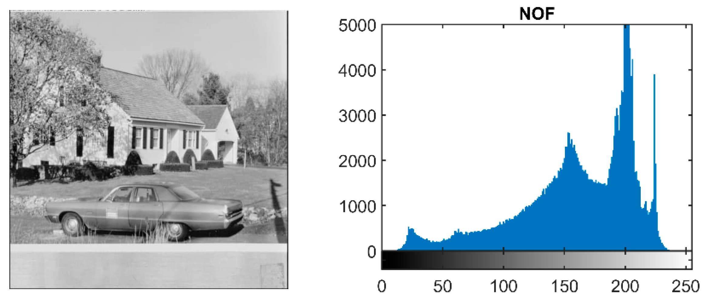
Here, the effect of filtering using their respective histograms is discussed. Figure 1 displays a non-filtered (NOF) grayscale image of 512 × 512 pixels with its histogram. The x-axis represents 256 gray levels from 0 to 255, and the y-axis represents the number of pixels of each gray level in the image.

Figure 1.
Non-filtered image and its histogram.
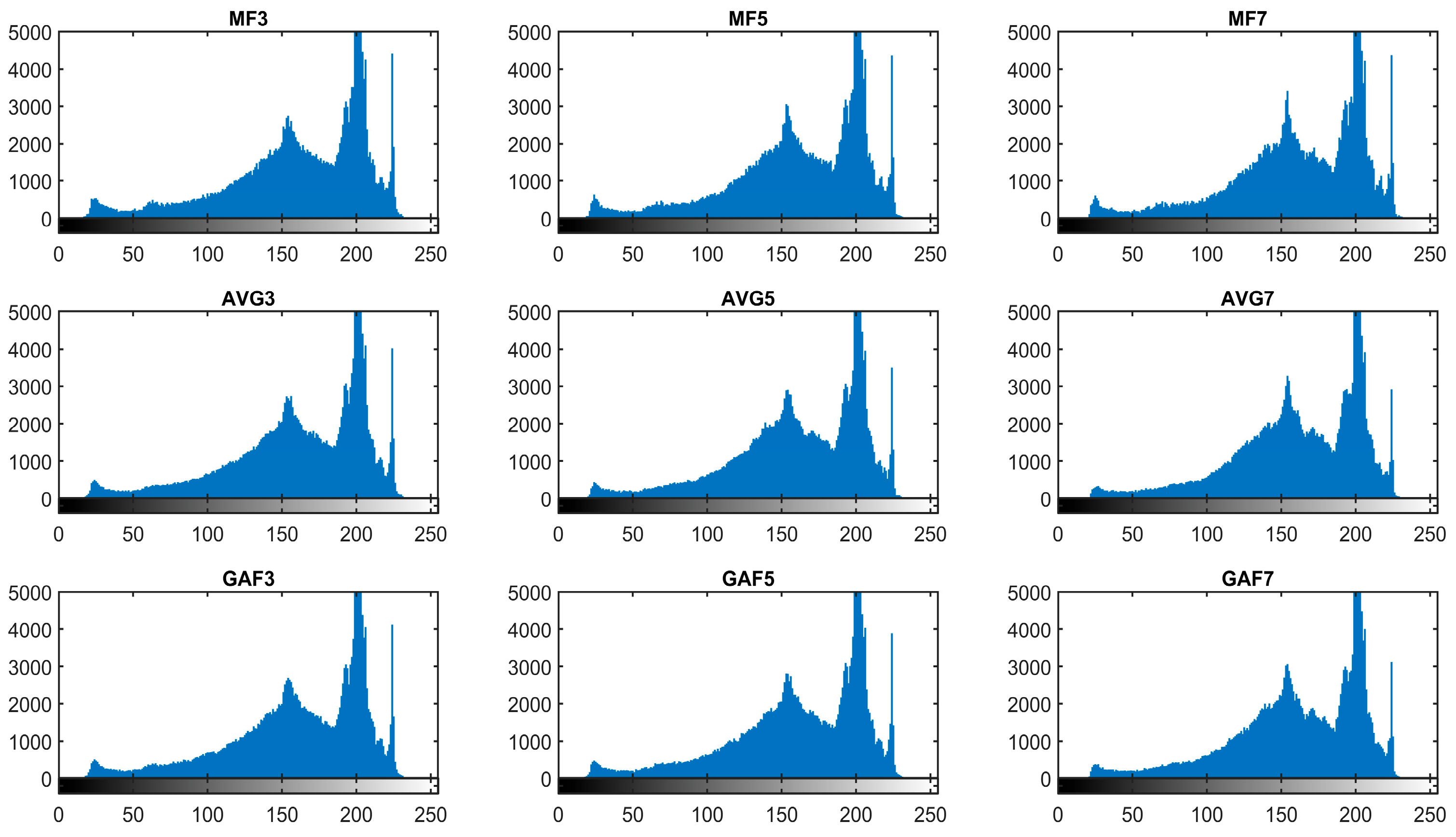
In Figure 2, histograms of the median, averaging, and Gaussian-filtered images are displayed. Median filters are represented as MEF3, MEF5, and MEF7 according to the filter’s window size, i.e., 3 × 3, 5 × 5, and 7 × 7, respectively. Similarly, according to the filter window size, Gaussian and averaging filters are abbreviated as GAF3, GAF5, GAF7, and AVF3, AVF5, and AVF7. There is no big visual difference in histograms; still, the peaks of histograms are comparatively smoother for averaging and Gaussian-filtered images.
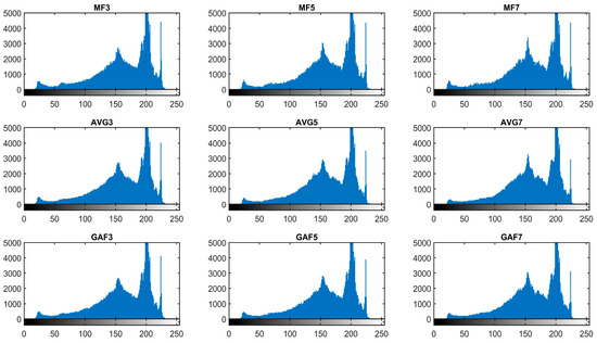
Figure 2.
Histograms of filtered images.
The unmodified elements of the residual arrays of fifteen thousand non-filtered images and filtered images of size 64 × 64 pixels are shown in Table 1. The number of unmodified elements decreases as the filter window size increases while revealing an intriguing symmetry in the modification patterns. The median filter has a higher number of unmodified elements compared to averaging and Gaussian filters. Furthermore, it is evident from Table 1 that detecting filtering with small kernel sizes presents a greater challenge compared to detecting filtering with larger kernel sizes. However, this fact is overruled in multiclass classification, especially on the small size and compressed images. The smoothing filter multiclass classification issue analysis is addressed in the next section. Further, some notable previous schemes of smoothing filtering are discussed.

Table 1.
Unmodified elements in non-filtered and filtered images residual arrays.
Some notable schemes to detect smoothing filtering are discussed here. Kirchner and Fridrich [4] analyzed the histogram bins in uncompressed images. They applied the Markov model in compressed images to detect the median filtering. This scheme works well on uncompressed images. To improve the detection performance on JPEG-compressed images, Chen et al. [5] suggested the popular scheme known as GLF (global and local feature set). Global features are extracted using the Markov model. Local features are considered pixel correlation. Agarwal et al. [6] further improved the performance by considering the first-, second-, and third-order difference arrays for better outcomes. The Markov model is applied to difference arrays to detect median filtering. Scheme [7] considered the higher significant bit-plane (HSB) from an 8-bit image to calculate co-occurrence statistics. This scheme is effective for the median, Gaussian, and averaging filtering detection. Gupta and Singhal [8] converted the spatial images into the DCT domain. Mean, variance, skewness, and kurtosis features classify non-filtered and median-filtered images. However, the scheme’s performance is not satisfactory. Kang and colleagues [9] applied the Autoregressive model of order ten to identify median filtering. Yang et al. [10] applied the 2D Autoregressive model on multiple residual arrays for robust performance. Rhee [11] used the Autoregressive model on each bit plane of an image separately to identify mean filtering, Gaussian filtering, and image resampling. The Autoregressive model results are found to be inferior to Markov-based schemes.
Chen et al. [12] first applied the CNN model to identify median filtering with marginal outcomes. Five convolutional layers are utilized in the network. Median filter residual images are used to train the network. Liu and researchers [13] applied their proposed CNN model after converting the image to the frequency domain using a discrete Fourier transform to detect median, Gaussian, and averaging filtering. In their CNN, there are only two convolutional layers and pooling layers, which may be the reason for inferior performance. Zhang et al. [14] suggested the CNN model to detect median, Gaussian, and averaging filtering. Two types of squeeze and excitation blocks are considered, i.e., Inception and ResNet. However, the computational cost is comparatively high. Yu and colleagues [15] conducted image pre-processing using various high-pass kernels. The proposed deep network contains four convolutional layers to detect median filtering. The existing scheme broadly followed two approaches. The first approach extracts features manually using the Markov or autoregressive models. Deep networks are exploited with different arrangements of layers with or without pre-processing steps in the second type of approach. Papers [16,17] utilized a Quaternion Convolutional Neural Network (QCNN) to detect median filtering in color images. The approach involves image pre-processing with median filter residual, expanding the output into four channels for QCNN input, utilizing quaternion convolution for multi-channel integration, and implementing a quaternion pooling layer to enhance feature extraction from an image’s three color channels effectively. In [18], the AlexCaps network is introduced, combining AlexNet with Capsule network elements. A shallow conventional convolutional neural network extracts essential features from input images. The capsule network layer also employs dynamic routing for precise spatial information capture and accurate predictions.
A deep network-based scheme outperforms the manual approach because deep networks can learn more complex relationships between the images’ features, allowing them to better distinguish between smoothed and non-smoothed images. In this paper, a deep network-based method is proposed, which has a better detection capability and moderate computational cost, accentuating the significance of symmetry in refining the discernment between different image smoothing effects. The main contributions of this paper are as follows:
- A hybrid scheme based on the deep network and feature extraction is proposed to detect median, Gaussian, and averaging filtering.
- A reduced number of kernels are utilized in the convolutional layers to minimize computational overhead.
- Accumulating trained deep network features by applying three distinct optimizers enhances detection accuracy.
- The global average pooling layer is considered in the network to extract promising features. No downsizing is performed in the CNN to exploit the whole statistical fingerprints of filtering.
- Support vector machine multiclass classifiers with linear and quadratic kernels are applied to classify from combined feature vectors.
- The proposed scheme yields superior outcomes to current methods for small-sized and compressed images.
2. The Proposed Scheme
Digital images are a quick representation of information. Fake images are created to spread false information rapidly. The memories of fake images also have long-term traces in the brain, like real images. Fake images are produced using many operations to fool people. In this paper, smoothing operations, i.e., median filtering, Gaussian filtering, and averaging filtering, are detected using a lightweight deep network. Three filter window sizes are considered, i.e., 3 × 3, 5 × 5, and 7 × 7. Overall, ten classes need to be classified as non-filtered and filtered images. Commonly, peak signal-to-noise ratio (PSNR) and structural similarity index measure (SSIM) [19] are used to evaluate the quality of images. The SSIM can be defined as follows:
where and are the two images being compared.
and are the means of and .
and are the standard deviations of and .
is the cross-covariance between and .
and are small constants to prevent division by zero.
To simplify the details, normalized SSIM is considered with the SSIM value ranging from 0 to 1. The higher value of SSIM is assumed for a good-quality image. In our study, it is found that SSIM is more suitable for understanding the effect of different types of filtering. Figure 3 displays non-filtered and filtered uncompressed images with their corresponding SSIM value. A non-filtered color image and its corresponding grayscale image are displayed in the first row. The second image in the first row is considered as the reference image for calculating the SSIM value. Second-, third-, and fourth-row images are median filtered, averaging filtered, and Gaussian filtered. The visible effect on the averaging and median filtered image is more apparent than the Gaussian-filtered image. SSIM values are higher for Gaussian-filtered images. Averaging filtered image processed with 7 × 7 window size mean filter has least SSIM value, i.e., 0.8047. Figure 4 displays the mean value of SSIM for uncompressed and compressed 1000 images. It can be seen in Figure 4 that the SSIM value of Gaussian-filtered images is highest. Also, the SSIM value of uncompressed images is more elevated than that of compressed images. The experimental results also reflect the SSIM value behavior on filtered images.
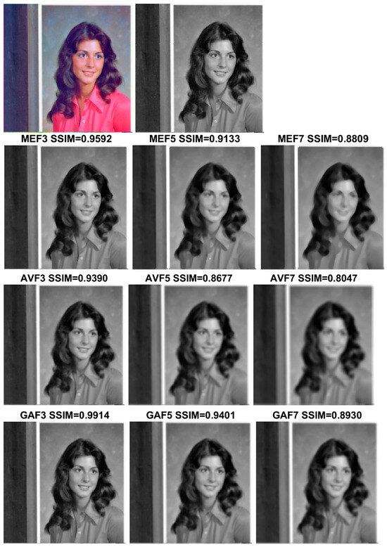
Figure 3.
Non-filtered and filtered images with their respective SSIM.

Figure 4.
SSIM values of filtered images.
The mean value of entropy and the standard deviation are displayed in Table 2 for one thousand uncompressed and compressed images. However, entropy and standard deviation values cannot distinguish between non-filtered and filtered images. SSIM is better able to identify image filtering effects.
Table 2.
Entropy and standard deviation of images.
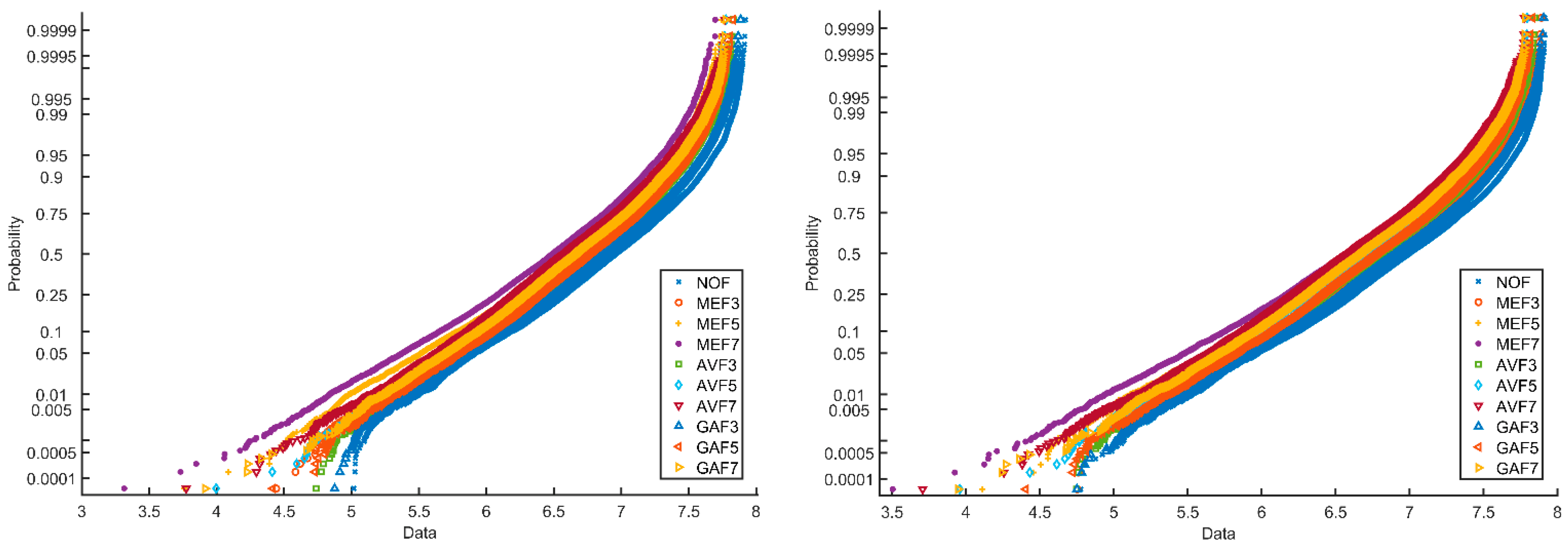
Figure 5 shows the probability plot of entropy normal distribution for one thousand images of size of 64 × 64. Ten categories of images, i.e., non-filtered (NOF) images, median filtered images, averaging filtered images, and Gaussian filtered images processed by filter sizes, 3 × 3, 5 × 5, and 7 × 7, are considered. There is some overlapping in the distribution of entropy values of uncompressed images in the first figure. This is due to the small image sizes, particularly 64 × 64. The gap between the curves is decreased, and overlapping is increased while considering JPEG compression, as seen in the second plot of Figure 5. The characteristics of these plots are reflected in the experimental analysis.
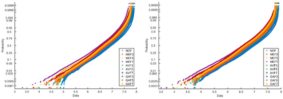
Figure 5.
Probability plot of entropy normal distribution of images.
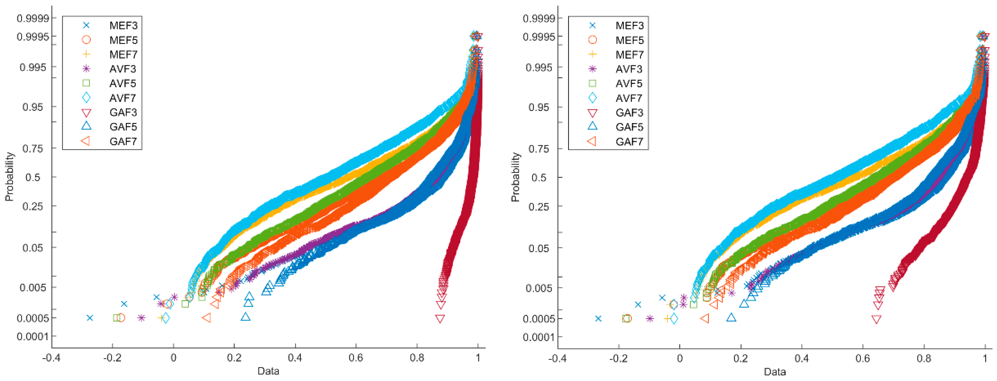
While considering SSIM values, the difference between uncompressed and compressed filtered images can be better visualized. In Figure 6, a probability plot of SSIM value normal distribution is displayed of 64 × 64 uncompressed (left figure) and compressed images (right figure). Convolutional neural networks with different optimizers and traditional SVM classifiers are utilized to overcome this issue.
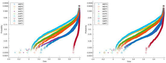
Figure 6.
Probability plot of SSIM value normal distribution of images.
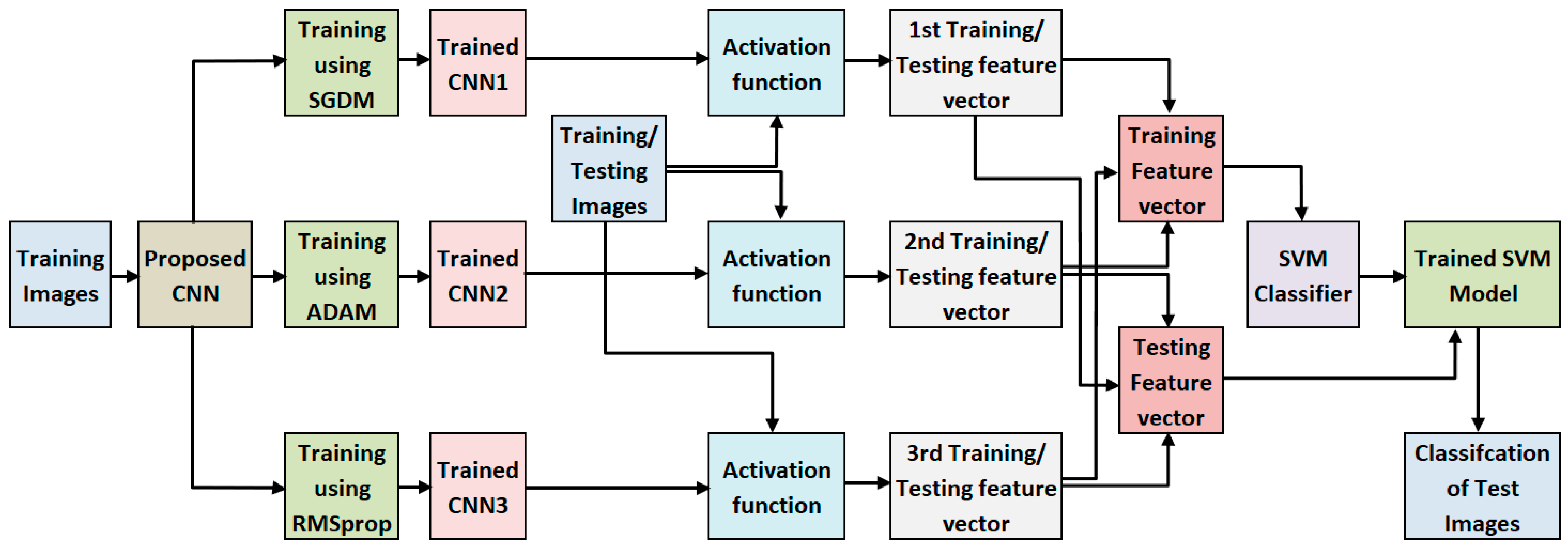
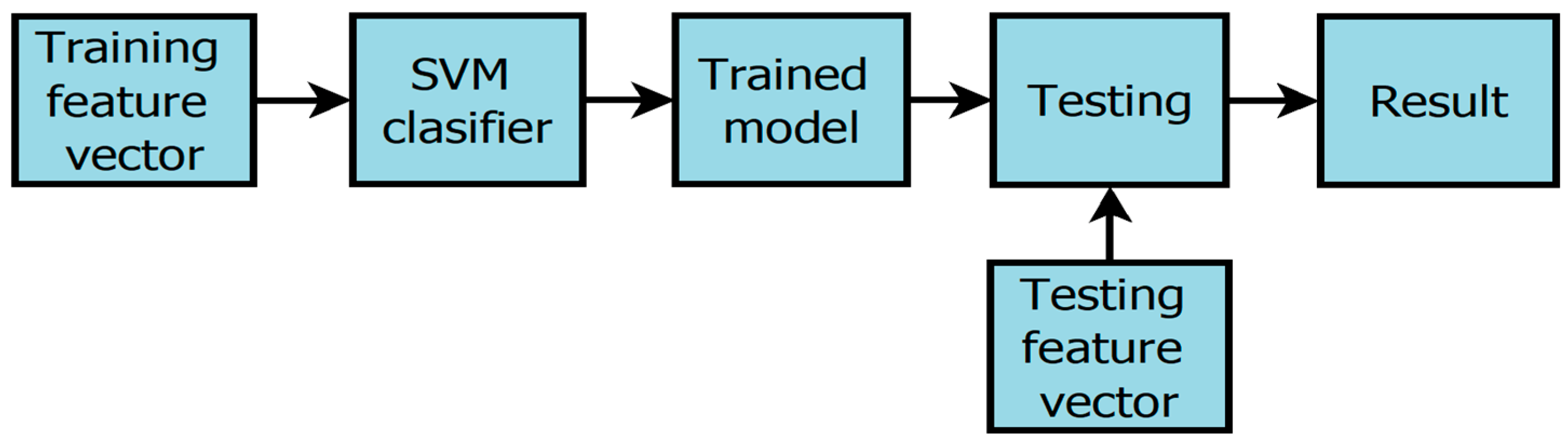
The framework of the suggested approach is depicted in Figure 7. To train the proposed CNN, a set of training images is utilized with three distinct optimizers. Subsequently, features are extracted using an activation function. Training feature vectors are obtained from the training images while testing feature vectors are derived from the testing images. Furthermore, we employ an SVM classifier to categorize various classes within the testing images. The subsequent sections delve into a comprehensive discussion on CNN, feature vector extraction, and the classification process.
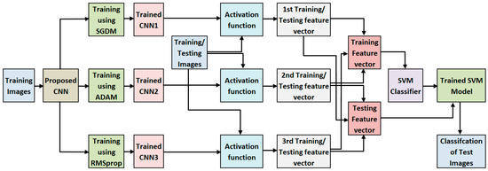
Figure 7.
Framework of proposed Scheme.
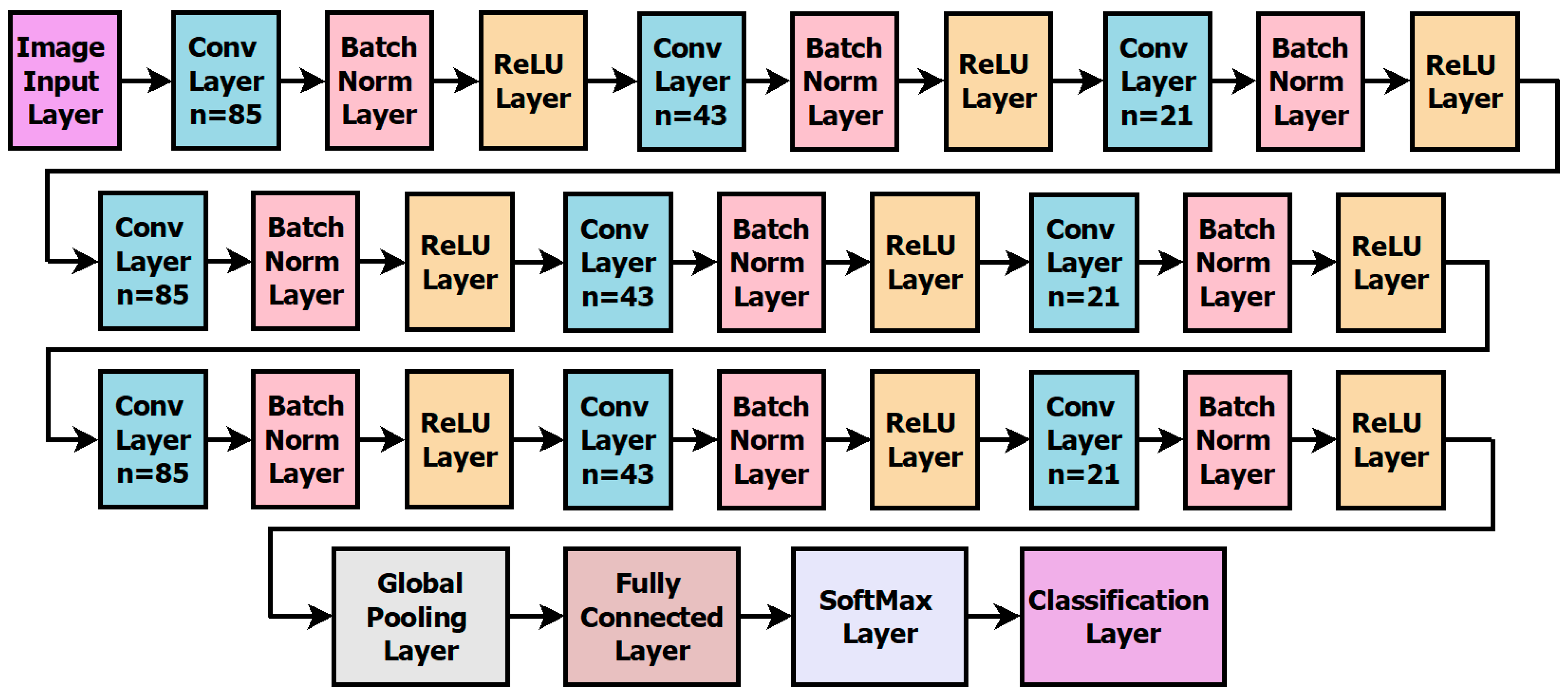
The proposed Convolutional Neural Network (CNN) is illustrated in Figure 8; a total of nine convolutional layers are employed. Following each convolutional layer is a batch normalization layer and a rectifier linear unit (ReLU) layer. The specific configurations for the kernels in these convolutional layers are as follows: 85, 45, 21, 85, 45, 21, 85, 45, and 21 for the first to ninth convolutional layers, respectively. Extensive experimental analysis has been conducted by exploring configurations with more than nine convolutional layers and a more significant number of kernels. Surprisingly, this exploration did not yield any improvement in detection accuracy; in fact, it decreased detection accuracy. The final ReLU layer of the CNN is succeeded by a global average pooling layer, a fully connected layer, a softmax layer, and a classification layer. Compared to previous approaches, the proposed CNN offers a computational advantage due to the reduced number of network elements. The training process involves thirty-five epochs. Furthermore, different mini-batch sizes are considered based on the image size, with 200 for 64 × 64 size images and 100 for 32 × 32 size images.
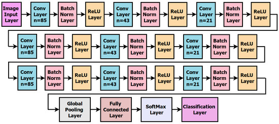
Figure 8.
Layout of proposed deep network.
Additionally, the proposed network undergoes training using three distinct optimization methods: stochastic gradient descent with momentum (SGDM) optimization, adaptive moment (Adam) optimization, and root mean squared propagation (RMSprop) optimization. Interestingly, when we compare the performance of these three optimization methods, there is no substantial difference in network performance. However, the network’s performance is significantly enhanced when we combine the outputs from these three networks. This is achieved by extracting features from the trained networks, thereby harnessing the advantages of all three optimization methods. A similar phenomenon has been observed in the context of two-operator series manipulation detection [20]. The activation function is applied to extract these features from the global average pooling layer of the trained network, as depicted in Figure 9.
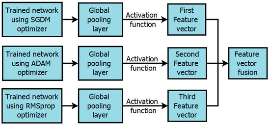
Figure 9.
Features extraction process from three trained networks.
Learned features are derived from all three of the trained networks. These extracted features are then concatenated, creating a feature vector, which possesses a dimensionality of 63 for each image. This process is systematically applied to all images within the training dataset. Subsequently, a Support Vector Machine (SVM) classifier is employed on these training feature vectors to generate a well-trained classification model. It is worth noting that numerous classifiers were evaluated, but the SVM with a quadratic kernel emerged as the most effective choice. This trained SVM model is subsequently utilized to classify images within the testing dataset, as depicted in Figure 10. The collective feature set’s performance significantly improved compared to a single-trained network. A more detailed experimental analysis is presented in the following section for a comprehensive understanding of these findings.

Figure 10.
SVM model training and testing layout.
The proposed scheme underwent testing on a computer equipped with MATLAB software and GPU capabilities, featuring the following hardware configuration: NVIDIA GeForce RTX3070, Intel(R) Core (TM) i7-10700K CPU @ 3.80 GHz, and 32.0 GB of RAM. To gauge the training efficiency of the proposed CNN, as illustrated in Figure 8, the training times are documented in Table 3. These training times were recorded while employing three optimization methods: SGDM, Adam, and RMSprop. Notably, the information content of compressed images is inherently lower than that of uncompressed images. Consequently, the training times for compressed images are significantly reduced compared to their uncompressed counterparts. Similarly, smaller image sizes result in shorter training times. When using the Adam and RMSprop optimizers during training, the training time for 32 × 32 compressed images falls below one hour. The overall execution time of the proposed scheme, including feature extraction and SVM model training and testing, amounts to 173.8 min for 32 × 32 size compressed images, utilizing fifteen thousand training images for each class.
Table 3.
Network training time in minutes.
3. Experimental Analysis
Image forensics is a profound concern as images are primarily used in communication. The dissemination of erroneous information can easily mislead users. This study focuses on detecting smoothing filters, commonly employed to diminish the traces of image forgery. Four distinct datasets are utilized in our experimental analysis to ensure an impartial evaluation of our proposed approach: BOSSBase 1.01 [21], the NRCS [22], the UCID [23], and the Dresden [24]. A total of 5000 images were gathered from these datasets, with 2000 pictures taken from BOSSBase 1.01 and Dresden and 500 photos from NRCS and UCID. The focus was placed on the central elements of the 5000 images to standardize image sizes at 192 × 192 and 96 × 96 pixels. An additional set of 45,000 images, each measuring 64 × 64 pixels, was generated from the 192 × 192 images. Likewise, 45,000 images, each 32 × 32 pixels in size, were extracted from the 96 × 96 images. A random selection of 35,000 images was made from both sets of images. This research encompasses a total of ten classes, including NOF (non-filtered), MEF3, MEF5, MEF7 (median filtered), GAF3, GAF5, GAF7 (Gaussian filtered), and AVF3, AVF5, AVF7 (averaging filtered), with each class comprising 35,000 images. Fifteen thousand images are designated for training, five thousand for validation, and the remaining 15,000 for testing. The training dataset images are distinct from the testing dataset images. The results presented encompass both uncompressed images and JPEG-compressed images.
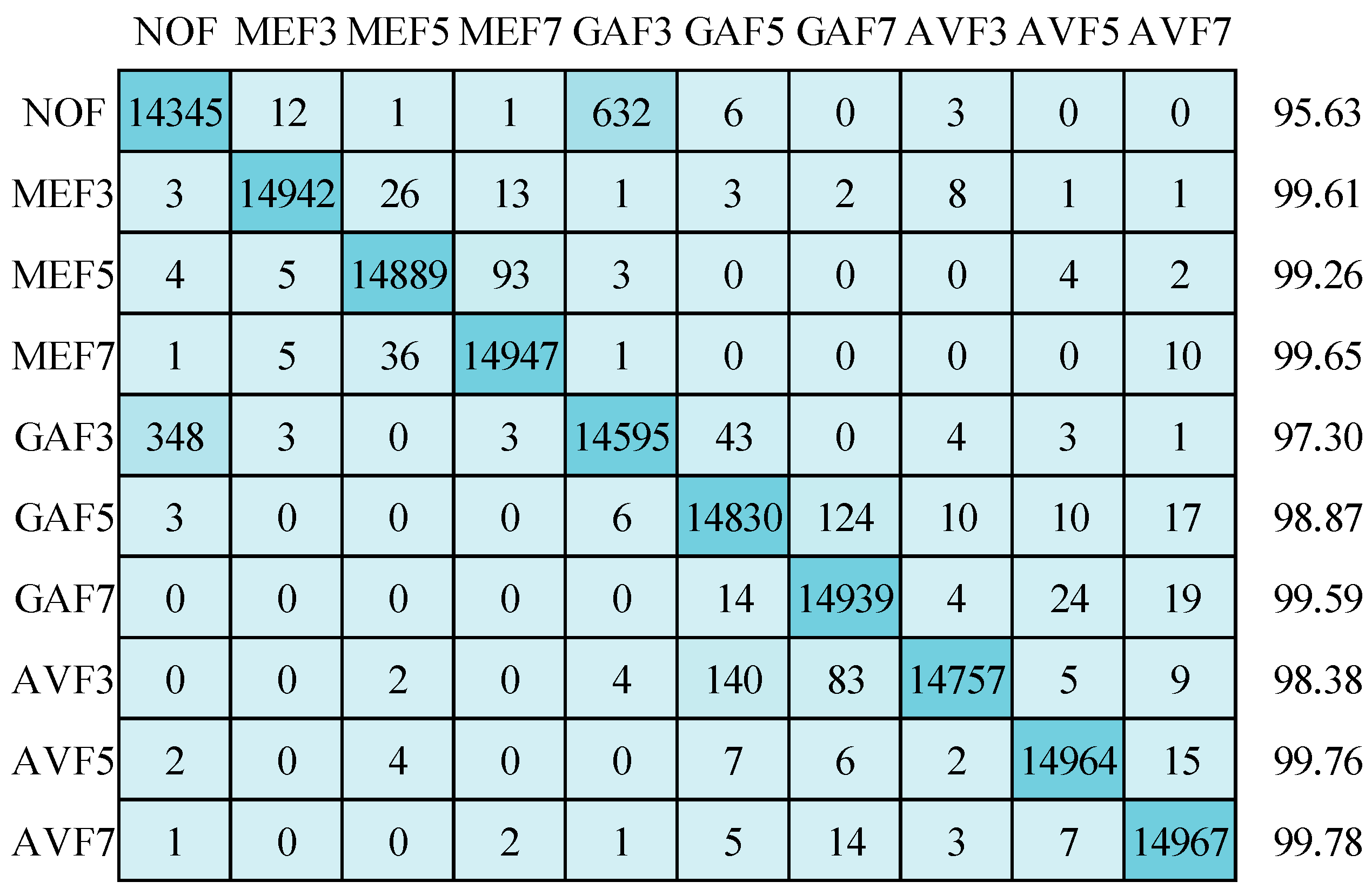
Now, the emphasis is on the results achieved by applying the suggested CNN depicted in Figure 8. These outcomes were attained using three distinct optimizers while operating on images standardized to a resolution of 64 × 64 pixels: Stochastic Gradient Descent with Momentum (SGDM), Adam, and RMSprop. Starting with the SGDM optimizer, the corresponding confusion matrix and detection accuracy for ten classes are showcased in Figure 11. Impressively, the mean detection accuracy stands at a notable 98.78%. However, it is essential to highlight the predominant issue of misclassification, primarily occurring between “non-filtered” (NOF) images and “Gaussian filtered 3 × 3 window size” (GAF3) images. Shifting our attention to the Adam optimizer, Figure 12 illustrates a mean detection accuracy of 98.39%. Within this context, a noteworthy observation is a misclassification within the NOF class, where 721 images are erroneously categorized as GAF3.
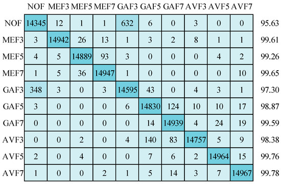
Figure 11.
Confusion matrix for image size 64 × 64 using SGDM optimizer.
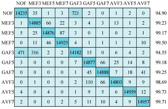
Figure 12.
Confusion matrix for image size 64 × 64 using Adam optimizer.
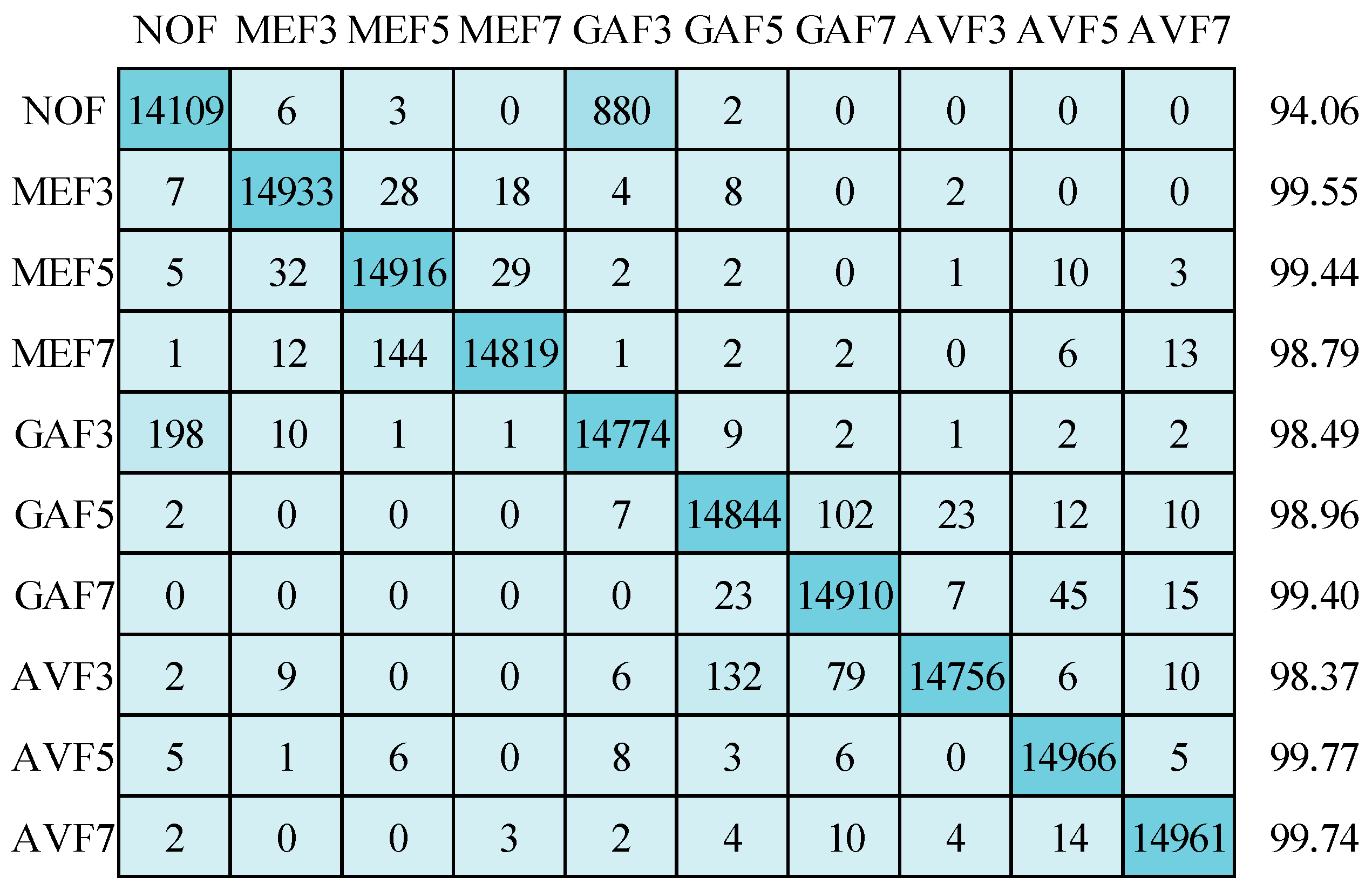
Conversely, the GAF3 class exhibits misclassification issues, with 471 images being misidentified as NOF and an additional 316 images incorrectly classified as MEF3. Figure 13 introduces the results obtained by applying the RMSprop optimizer, showcasing an impressive detection accuracy of 98.66% on 64 × 64 size testing set images. Once more, a significant misclassification concern emerges, with 880 images from the NOF class being inaccurately assigned to the GAF3 category. Lastly, it is worth noting that standard deviations for the detection accuracies across the ten categories are as follows: 1.36 for SGDM, 1.96 for Adam, and 1.69 for RMSprop optimizers. These standard deviations offer insights into the variation and consistency of the detection performance when employing different optimization techniques.
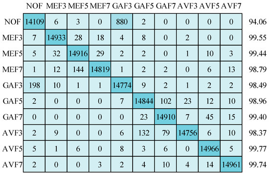
Figure 13.
Confusion matrix for image size 64 × 64 using RMSprop optimizer.
Figure 14 presents the confusion matrix and corresponding detection accuracy for the ten classes within the 32 × 32 size image testing dataset. When employing the SGDM optimizer, a mean detection accuracy of 96.53% is achieved. Notably, this accuracy, while commendable, is slightly lower than the results obtained with the 64 × 64 size image testing set. As in the case of the 64 × 64 testing set, the primary misclassifications are concentrated within the “non-filtered” (NOF) and “Gaussian filtered 3 × 3 window size” (GAF3) classes. It is worth highlighting that 309 images from the GAF5 class are erroneously assigned to the GAF7 class. In comparison, 256 images from the GAF5 class are misclassified as the AVF3 class.

Figure 14.
Confusion matrix for image size of 32 × 32 using SGDM optimizer.
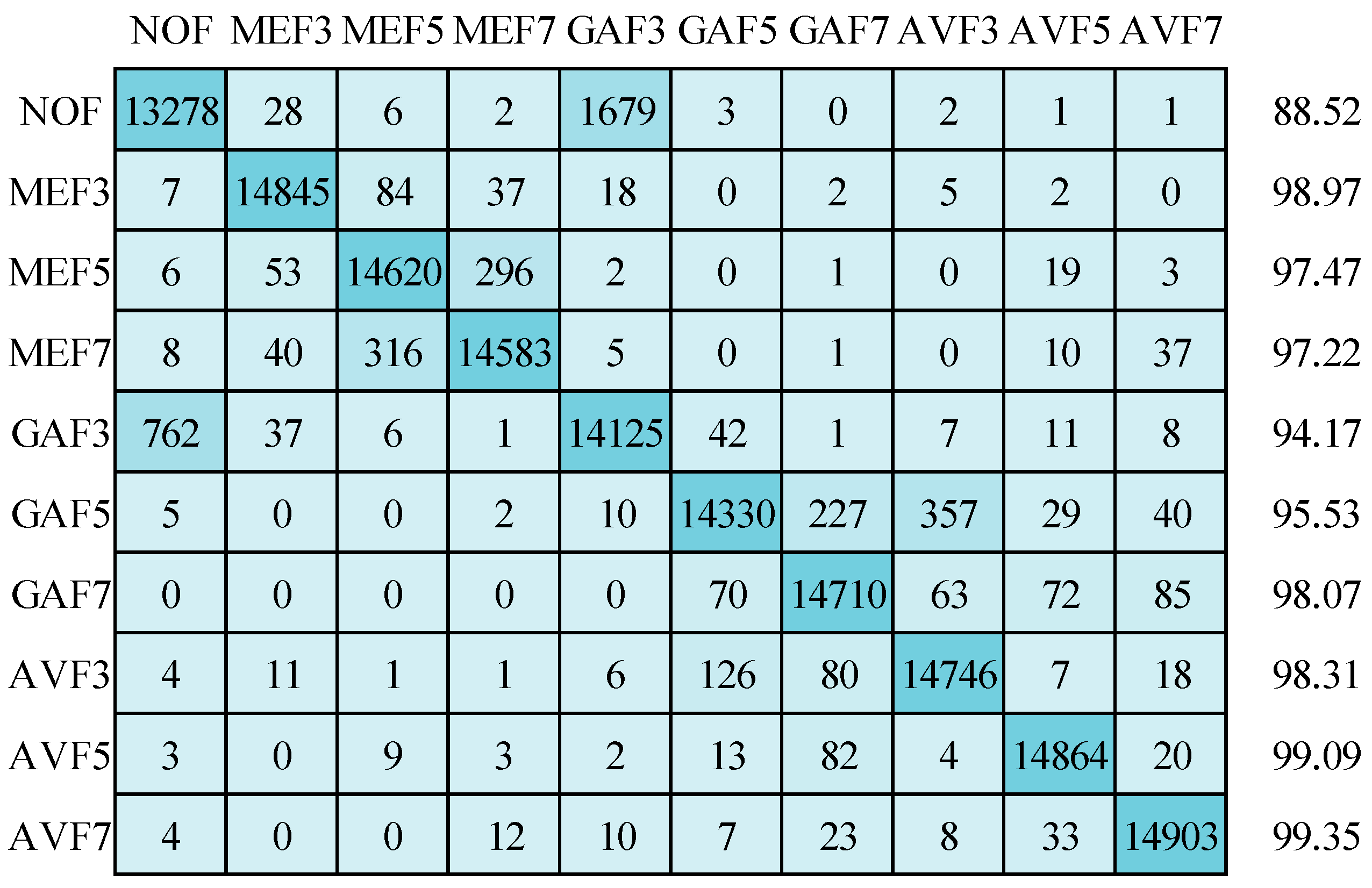
Moving on to the results obtained with the Adam optimizer, as depicted in Figure 15, a mean detection accuracy of 96.67% is achieved. The NOF class presents a significant challenge within this context, with 1679 images being misclassified as GAF3. Additionally, there is notable misclassification in the GAF5 class, with 227 and 357 images being incorrectly placed in the GAF7 and AVF3 classes, respectively. The NOF category exhibits the lowest detection accuracy, standing at 88.52%. It is primarily attributed to the close similarity in quality values between the NOF and GAF3 classes, as discussed in Figure 4. Notably, the Structural Similarity Index (SSIM) value is highest for the GAF3 class, indicating a close alignment with non-filtered images. Remarkably, the detection accuracy exceeds 99% for the AVF5 and AVF7 categories.
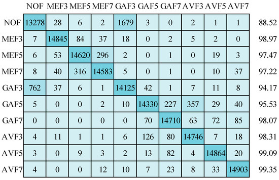
Figure 15.
Confusion matrix for image size 32 × 32 using Adam optimizer.
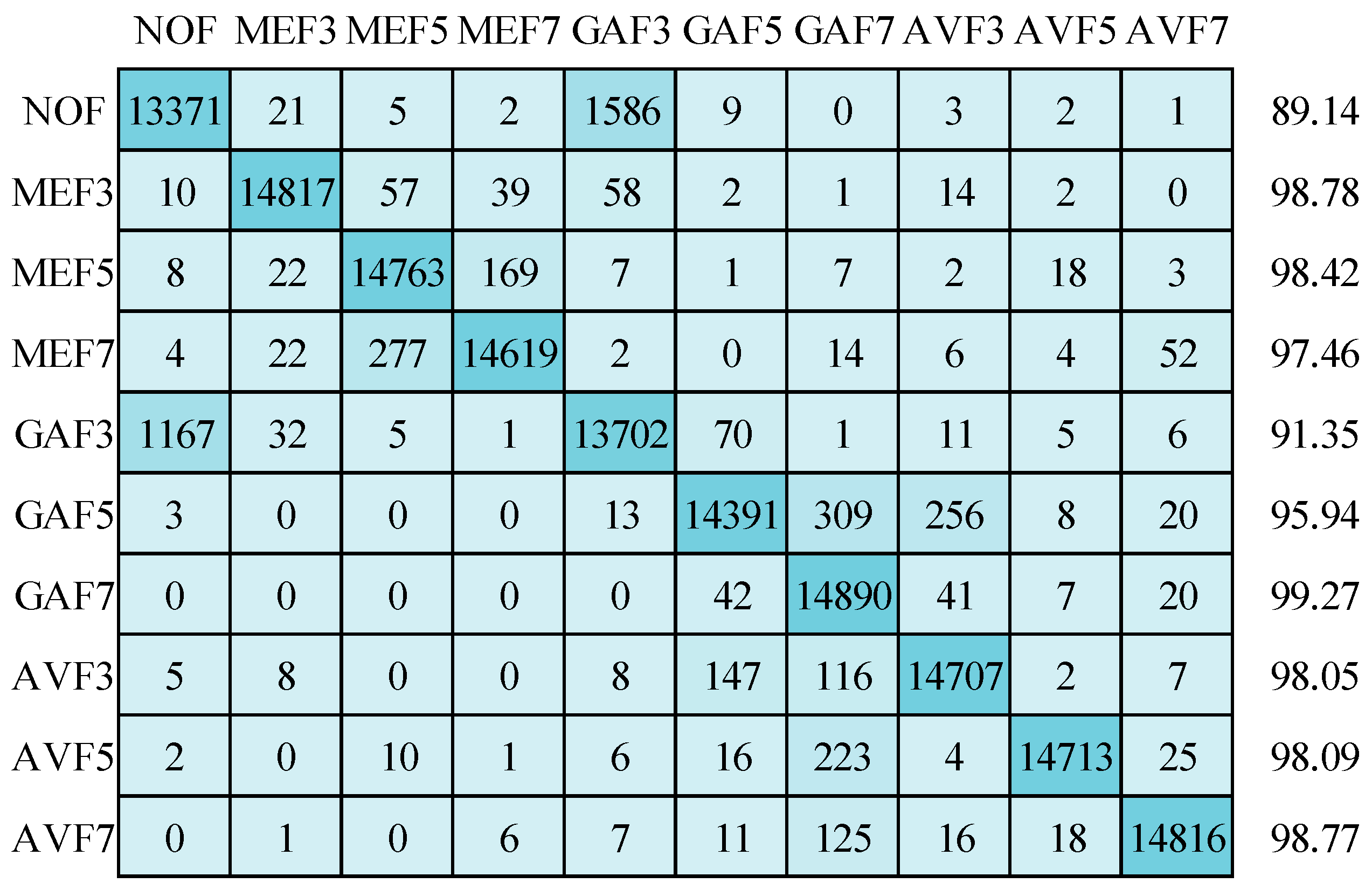
Figure 16 shows an average accuracy of 95.92% when employing the RMSprop optimizer. While this accuracy is slightly lower than what was achieved with the other two optimizers, the pattern of misclassifications differs from that observed with the Adam optimizer, particularly within the GAF7 and AVF3 categories.
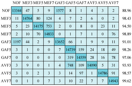
Figure 16.
Confusion matrix for image size of 32 × 32 using RMSprop optimizer.
Lastly, it is essential to consider the standard deviations for the detection accuracies across the ten categories, which are 3.47 for SGDM, 3.29 for Adam, and 3.67 for RMSprop optimizers. These standard deviations offer insights into the level of variation and consistency in detection performance when utilizing different optimization techniques.
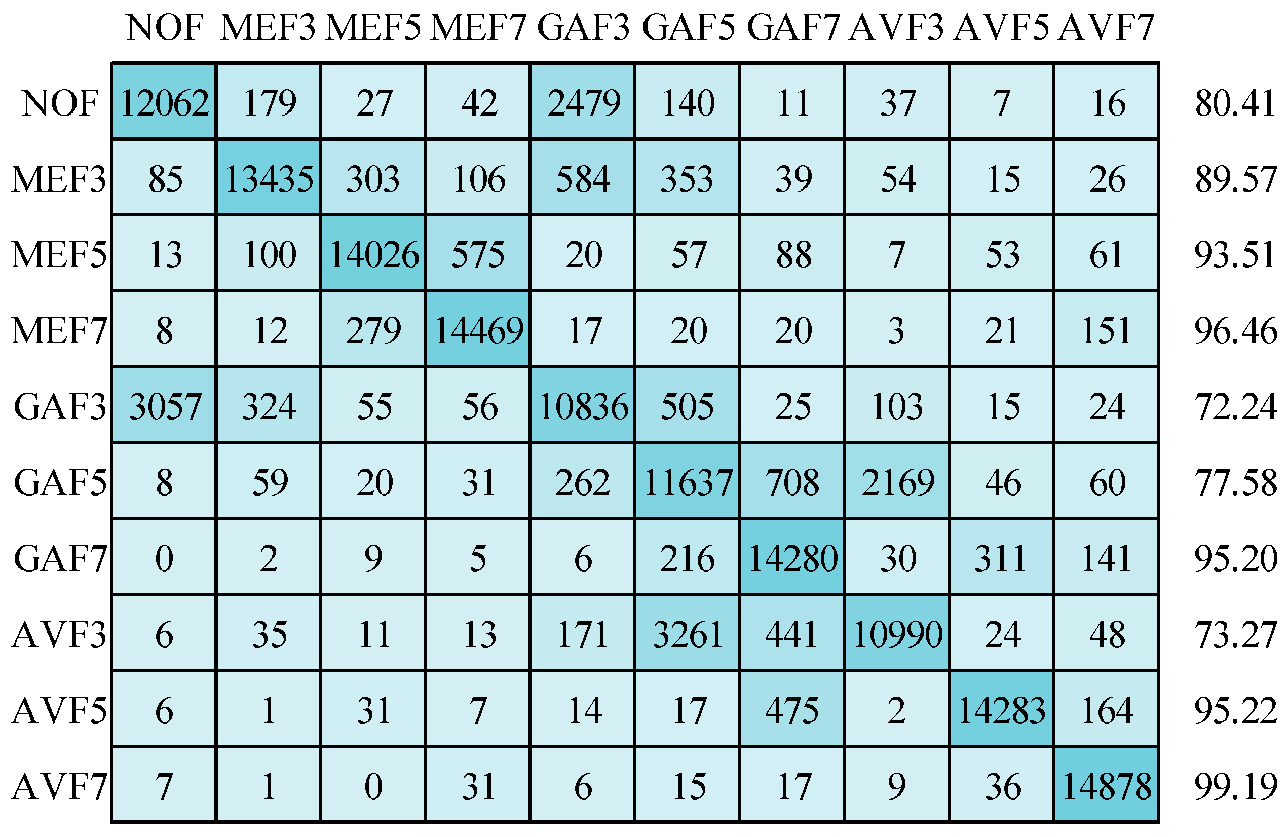
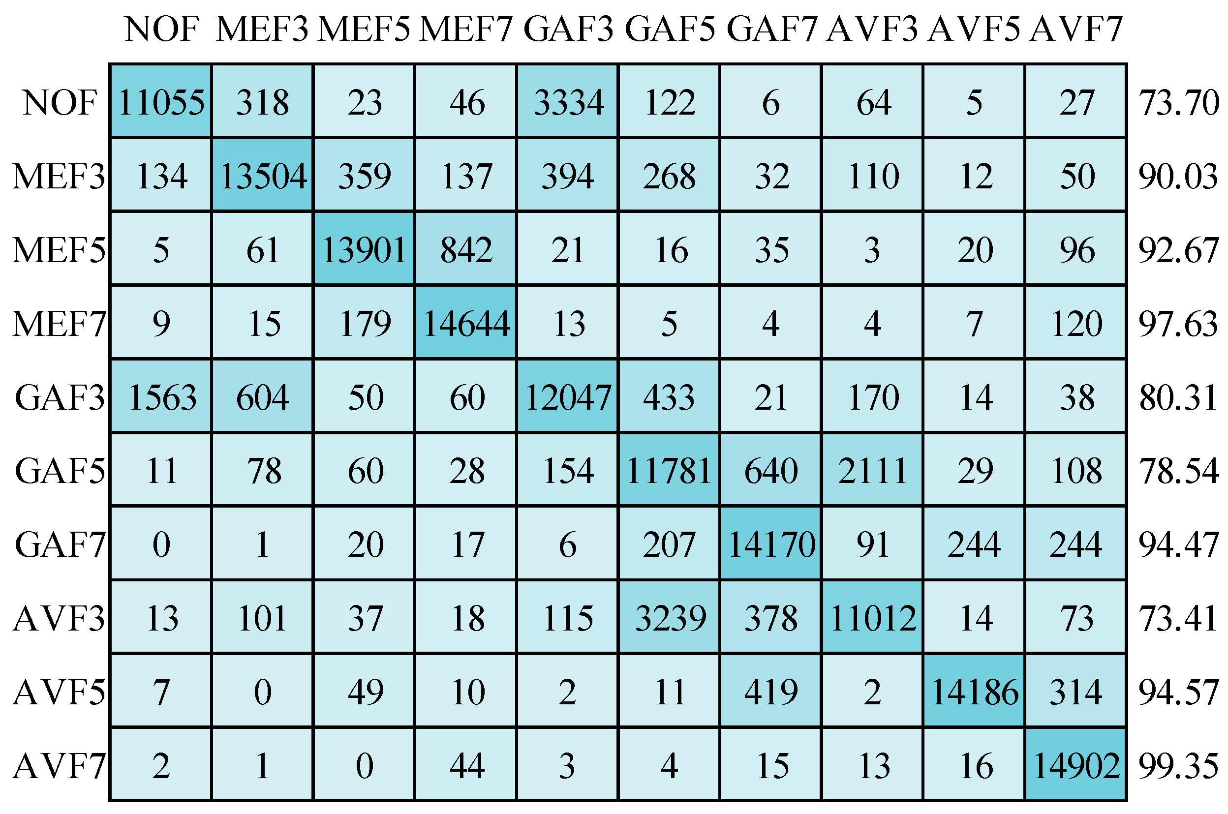
Now, the results are discussed on compressed image datasets. First, image sizes of 64 × 64 pixels are considered with JPEG compression quality 70. The mean detection accuracy is 87.26% while using the SGDM optimizer in training the deep network, as displayed in Figure 17. All classes are affected due to the compression artifacts. AVF7 class has the most minor compression effect and achieves 99.19% detection accuracy. GAF3 and AVF3 classes are highly affected, with detection accuracies of 72.24% and 73.27%, respectively. In Figure 18, the Adam optimizer provides 87.98% mean detection accuracy, slightly higher than the SGDM optimizer. Although, the confusion matrix pattern is similar to the SGDM optimizer confusion matrix. In Figure 19, the mean detection accuracy is 87.47% using the RMSprop optimizer in training. Here, 73.41% and 73.70% for the AVF3 and NOF categories are the least detection accuracies. AVF7 class has the best accuracy, i.e., 99.35%. The standard deviations for detection accuracies of ten types are 10.32, 9.92, and 9.97 for SGDM, Adam, and RMSprop optimizers, respectively. The standard deviation increases when the image size decreases, and compression is applied.
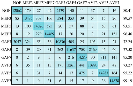
Figure 17.
Confusion matrix for image size of 64 × 64 with JC = 70 using SGDM optimizer.
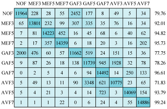
Figure 18.
Confusion matrix for image size of 64 × 64 with JC = 70 using Adam optimizer.
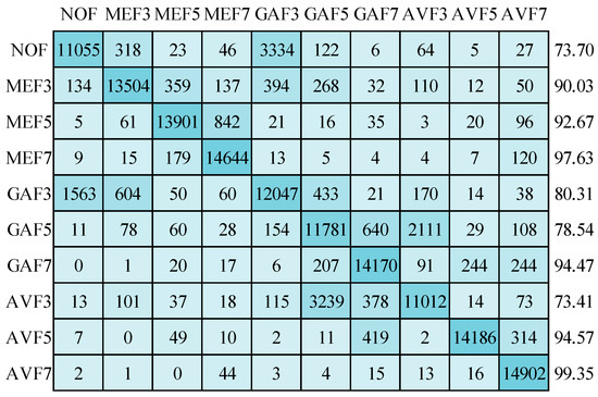
Figure 19.
Confusion matrix for image size of 64 × 64 with JC = 70 using RMSprop optimizer.
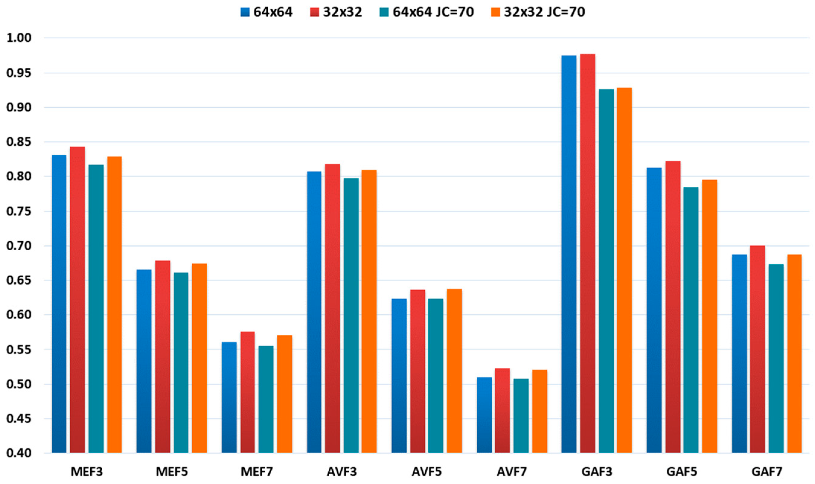
The results for small images of size 32 × 32 pixels JPEG compressed (JC = 70) are displayed in Table 4. The mean detection accuracies (MDAC) are 77.02%, 77.21%, and 77.33% while using SGDM, Adam, and RMSprop optimizers in training the deep network. The detection accuracy falls due to the small size of images and JPEG compression compared to the previous result discussion. The features are extracted from the trained networks to boost the performance, as shown in Figure 9 and Figure 10. There is a significant improvement in detection accuracy while using SVM with linear and quadratic kernels. Also, classification accuracy distribution is better when using the proposed CNN with the SVM classifier. The standard deviations for detection accuracies of the ten categories are 15.08, 15.99, 13.76, 13.05, and 13.09 for SGDM, Adam, RMSprop optimizers, SVM linear, and SVM quadratic classifiers, respectively.
Table 4.
Detection accuracy for 32 × 32 size compressed images.
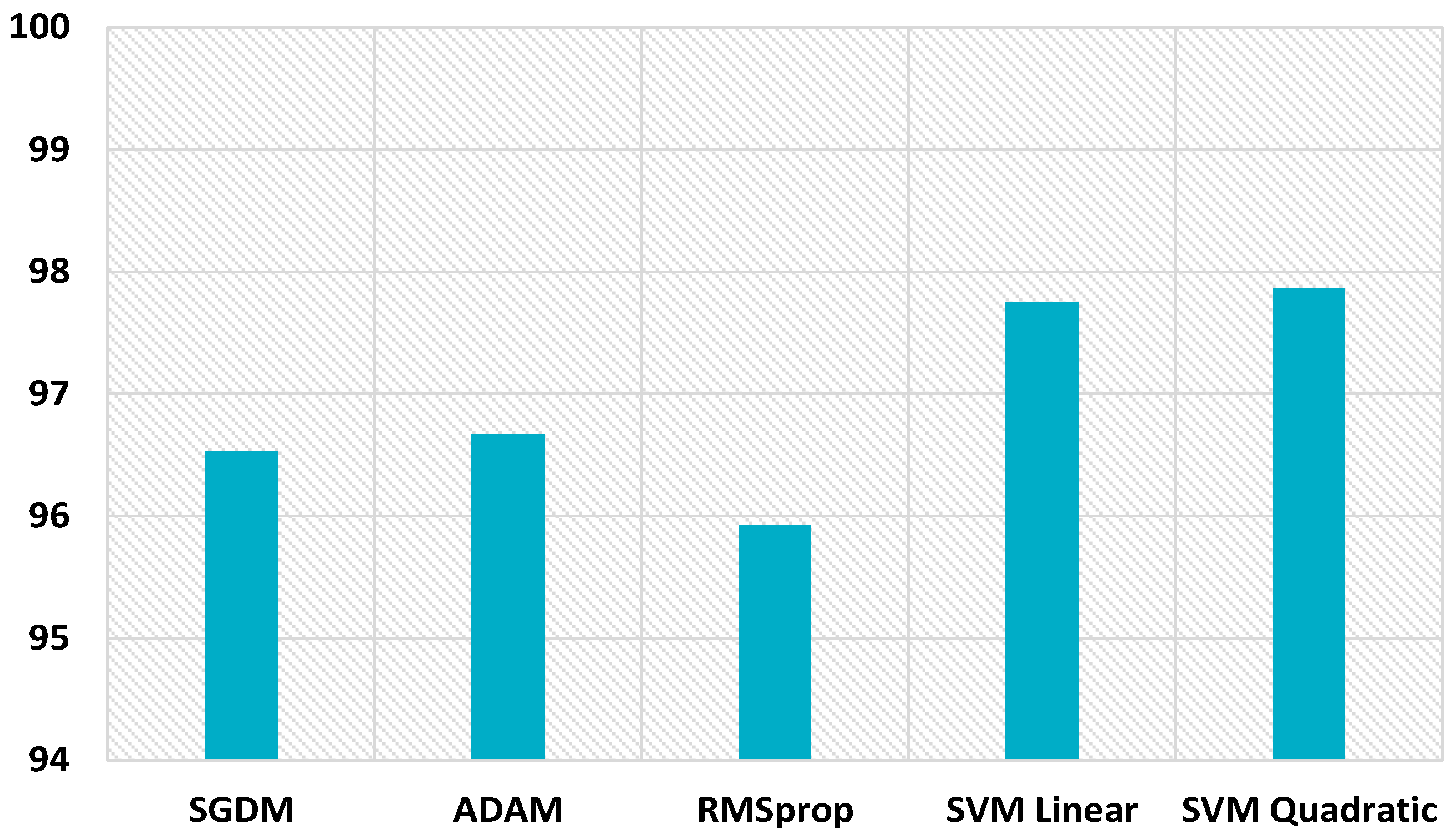
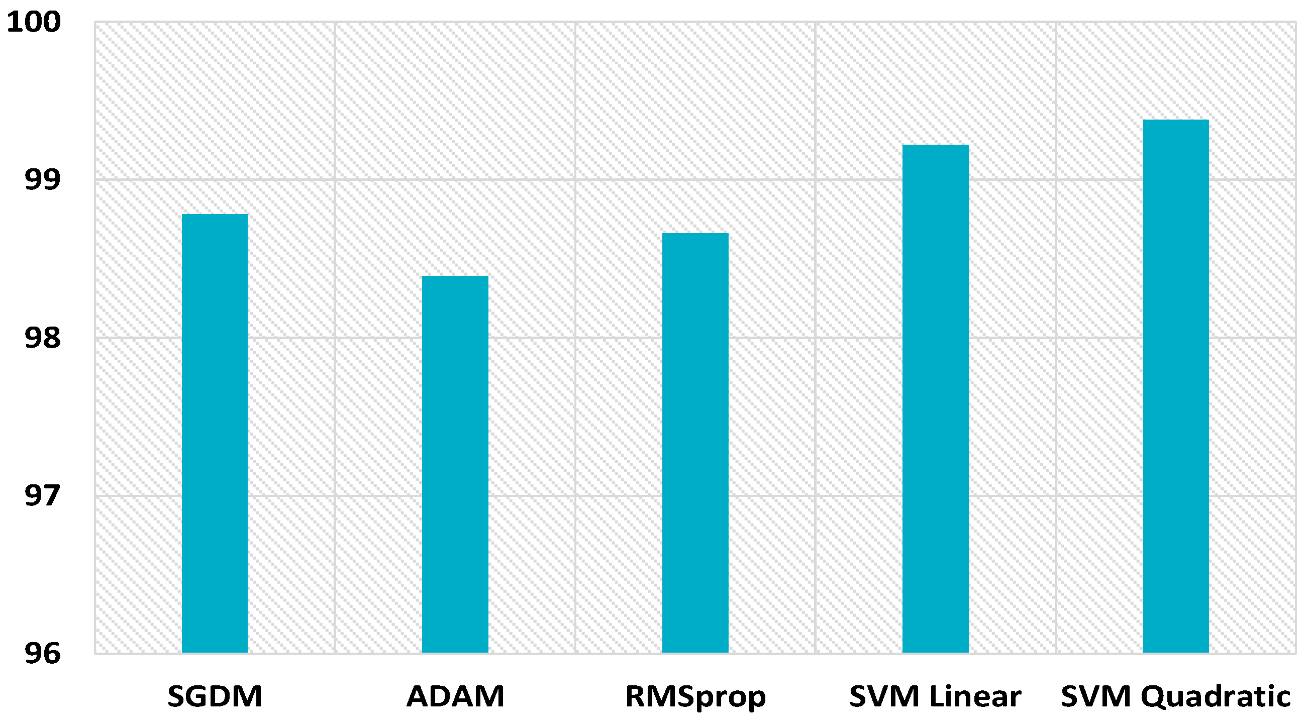
The proposed scheme also boosts the performance for uncompressed images of size 32 × 32, as displayed in Figure 20. The hybrid feature set gives better performance with the SVM linear kernel and SVM quadratic kernel, i.e., 97.75% and 97.86%, respectively, which highlights the inherent symmetry in the discernment of image smoothing. While only CNN gave 96.53%, 96.67, and 95.92% detection accuracies with SGDM, Adam, and RMSprop optimizers. The proposed scheme improves the detection accuracy for uncompressed images of size 64 × 64, as shown in Figure 21. The hybrid feature set achieves better performance with SVM linear kernel and SVM quadratic kernel, i.e., 99.22% and 99.38%, respectively. CNN gives 98.78%, 98.39, and 98.66% detection accuracies with SGDM, Adam, and RMSprop optimizers. The proposed scheme performance for 64 × 64 JPEG compressed images (JC = 70) is displayed in Figure 22. The combined feature set of size 63 provides superior results. The detection accuracies are 89.74% and 89.96% while using the SVM linear kernel and SVM quadratic kernel. CNN provides inferior results, i.e., 87.26%, 87.98, and 87.47% detection accuracies with SGDM, Adam, and RMSprop optimizers.
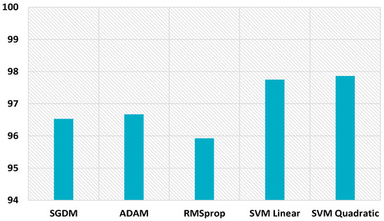
Figure 20.
MDAC for 32 × 32 size images.

Figure 21.
MDAC for 64 × 64 size uncompressed images.
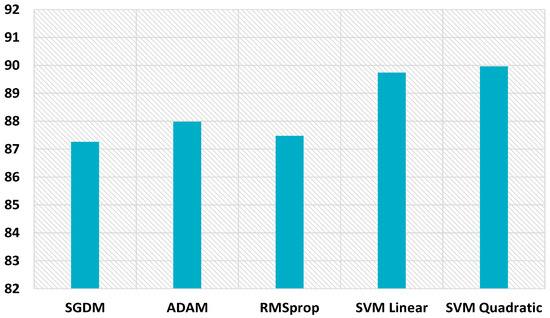
Figure 22.
MDAC for 64 × 64 size compressed images.
The proposed scheme is compared with other popular schemes, as displayed in Table 5. There is a significant improvement in detection accuracy while using the proposed method. The detection accuracy is superior for both compressed and uncompressed images. The proposed scheme achieves 89.96% detection accuracy for an image size of 64 × 64 and JPEG compression (JC = 70). The proposed scheme’s computational cost is low compared to techniques [13,14] based on deep learning.
Table 5.
Comparison of the detection accuracy with other schemes.
4. Conclusions
Genuine images have been exploited to create convincingly deceptive fake photos and videos, prompting the need for image forensics. In this paper, a novel scheme for identifying smoothing operators and leveraging the advantages of three optimizers to enhance detection capabilities while emphasizing symmetry in the analysis has been introduced. The proposed scheme is adept at distinguishing three distinct types of smoothing filters and their corresponding filter window sizes, particularly excelling in the detection of averaging, Gaussian, and median filtering in low-resolution images. A comprehensive image quality metric analysis was conducted, and the experimental results substantiated the findings. An exhaustive investigation, including various scenarios, demonstrated that the proposed scheme had superior performance compared to previous methods. The proposed scheme achieved remarkable detection accuracy, with rates reaching 99.38% and 97.86% for uncompressed 64 × 64 and 32 × 32 images, and the proposed scheme maintained strong performance with rates of 89.96% and 80.07% for 64 × 64 and 32 × 32 JPEG-compressed images at a quality factor of 70.
Author Contributions
Conceptualization, S.A. and K.-H.J.; software, S.A.; validation, K.-H.J.; formal analysis, S.A.; investigation, S.A.; resources, S.A.; data curation, K.-H.J.; writing—original draft preparation, S.A.; writing—review and editing, K.-H.J.; visualization, S.A.; supervision, K.-H.J.; project administration, K.-H.J.; funding acquisition, K.-H.J. All authors have read and agreed to the published version of the manuscript.
Funding
This research was supported by the Brain Pool program funded by the Ministry of Science and ICT through the National Research Foundation of Korea (2019H1D3A1A01101687) and the Basic Science Research Program through the National Research Foundation of Korea (NRF) funded by the Ministry of Education (2021R1I1A3049788).
Data Availability Statement
The datasets used in this paper are publicly available, and their links are provided in the reference section.
Acknowledgments
We thank the anonymous reviewers for their valuable suggestions that improved the quality of this article.
Conflicts of Interest
The authors declare no conflict of interest.
References
- Nam, S.H.; Ahn, W.; Mun, S.M.; Park, J.; Kim, D.; Yu, I.J.; Lee, H.K. Content-Aware Image Resizing Detection Using Deep Neural Network. In Proceedings of the 2019 IEEE International Conference on Image Processing (ICIP), Taipei, Taiwan, 22–25 September 2019; IEEE: Piscataway, NJ, USA, 2019; pp. 106–110. [Google Scholar] [CrossRef]
- Birajdar, G.K.; Mankar, V.H. Blind image forensics using reciprocal singular value curve based local statistical features. Multimed. Tools Appl. 2018, 77, 14153–14175. [Google Scholar] [CrossRef]
- Bi, X.L.; Qiu, Y.M.; Xiao, B.; Li, W.S.; Ma, J.F. Histogram Equalization Detection Based on Statistical Features in Digital Image. Jisuanji Xuebao/Chin. J. Comput. 2021, 44, 292–303. [Google Scholar] [CrossRef]
- Kirchner, M.; Fridrich, J. On detection of median filtering in digital images. In Media Forensics and Security II; Memon, N.D., Dittmann, J., Alattar, A.M., Delp, E.J., III, Eds.; SPIE: Bellingham, WA, USA, 2010; p. 754110. [Google Scholar] [CrossRef]
- Chen, C.; Ni, J.; Huang, J. Blind Detection of Median Filtering in Digital Images: A Difference Domain Based Approach. IEEE Trans. Image Process. 2013, 22, 4699–4710. [Google Scholar] [CrossRef] [PubMed]
- Agarwal, S.; Chand, S.; Skarbnik, N. SPAM revisited for median filtering detection using higher-order difference. Secur. Commun. Netw. 2016, 9, 4089–4102. [Google Scholar] [CrossRef]
- Agarwal, S.; Jung, K.-H. HSB-SPAM: An Efficient Image Filtering Detection Technique. Appl. Sci. 2021, 11, 3749. [Google Scholar] [CrossRef]
- Gupta, A.; Singhal, D. A simplistic global median filtering forensics based on frequency domain analysis of image residuals. ACM Trans. Multimed. Comput. Commun. Appl. 2019, 15, 1–23. [Google Scholar] [CrossRef]
- Kang, X.; Stamm, M.C.; Peng, A.; Liu, K.J.R. Robust Median Filtering Forensics Using an Autoregressive Model. IEEE Trans. Inf. Forensics Secur. 2013, 8, 1456–1468. [Google Scholar] [CrossRef]
- Yang, J.; Ren, H.; Zhu, G.; Huang, J.; Shi, Y.-Q. Detecting median filtering via two-dimensional AR models of multiple filtered residuals. Multimed. Tools Appl. 2018, 77, 7931–7953. [Google Scholar] [CrossRef]
- Rhee, K.H. Forensic Detection Using Bit-Planes Slicing of Median Filtering Image. IEEE Access 2019, 7, 92586–92597. [Google Scholar] [CrossRef]
- Chen, J.; Kang, X.; Liu, Y.; Wang, Z.J. Median Filtering Forensics Based on Convolutional Neural Networks. IEEE Signal Process. Lett. 2015, 22, 1849–1853. [Google Scholar] [CrossRef]
- Liu, A.; Zhao, Z.; Zhang, C.; Su, Y. Smooth filtering identification based on convolutional neural networks. Multimed. Tools Appl. 2019, 78, 26851–26865. [Google Scholar] [CrossRef]
- Zhang, Y.; Yu, L.; Fang, Z.; Xiong, N.N.; Zhang, L.; Tian, H. An end-to-end deep learning model for robust smooth filtering identification. Future Gener. Comput. Syst. 2022, 127, 263–275. [Google Scholar] [CrossRef]
- Yu, L.; Zhang, Y.; Han, H.; Zhang, L.; Wu, F. Robust Median Filtering Forensics by CNN-Based Multiple Residuals Learning. IEEE Access 2019, 7, 120594–120602. [Google Scholar] [CrossRef]
- Wang, J.; Zhang, Y. Median Filtering Forensics Scheme for Color Images Based on Quaternion Magnitude-Phase CNN. Comput. Mater. Contin. 2020, 62, 99–112. [Google Scholar] [CrossRef]
- Wang, J.; Ni, Q.; Zhang, Y.; Luo, X.; Shi, Y.; Zhai, J.; Jha, S.K. Median Filtering Detection Based on Quaternion Convolutional Neural Network. Comput. Mater. Contin. 2020, 65, 929–943. [Google Scholar] [CrossRef]
- Duan, G.; Miao, J.; Huang, T. Median Filtering Detection of Small-Size Image Using AlexCaps-Network. In Digital Forensics and Watermarking. IWDW 2019; Lecture Notes in Computer Science; Springer: Cham, Switzerland, 2020; Volume 12022, pp. 126–140. [Google Scholar] [CrossRef]
- Wang, Z.; Bovik, A.C.; Sheikh, H.R.; Simoncelli, E.P. Image Quality Assessment: From Error Visibility to Structural Similarity. IEEE Trans. Image Process. 2004, 13, 600–612. [Google Scholar] [CrossRef] [PubMed]
- Agarwal, S.; Cho, D.-J.; Jung, K.-H. Detecting Images in Two-Operator Series Manipulation: A Novel Approach Using Transposed Convolution and Information Fusion. Symmetry 2023, 15, 1898. [Google Scholar] [CrossRef]
- Bas, P.; Filler, T.; Pevný, T. Break Our Steganographic System: The Ins and Outs of Organizing BOSS. In Information Hiding. IH 2011; Lecture Notes in Computer Science; Springer: Berlin/Heidelberg, Germany, 2011; Volume 6958, pp. 59–70. [Google Scholar] [CrossRef]
- USDA NRCS 2014. Natural Resources Conservation Service Photo Gallery, United States Department of Agriculture. Available online: http://plants.usda.gov/ (accessed on 21 February 2022).
- Schaefer, G.; Stich, M. UCID: An uncompressed color image database. In Storage and Retrieval Methods and Applications for Multimedia 2004; Yeung, M.M., Lienhart, R.W., Li, C.-S., Eds.; SPIE: Bellingham, WA, USA, 2003; pp. 472–480. [Google Scholar] [CrossRef]
- Gloe, T.; Böhme, R. The Dresden Image Database for Benchmarking Digital Image Forensics. J. Digit. Forensic Pract. 2010, 3, 150–159. [Google Scholar] [CrossRef]


Disclaimer/Publisher’s Note: The statements, opinions and data contained in all publications are solely those of the individual author(s) and contributor(s) and not of MDPI and/or the editor(s). MDPI and/or the editor(s) disclaim responsibility for any injury to people or property resulting from any ideas, methods, instructions or products referred to in the content. |
© 2023 by the authors. Licensee MDPI, Basel, Switzerland. This article is an open access article distributed under the terms and conditions of the Creative Commons Attribution (CC BY) license (https://creativecommons.org/licenses/by/4.0/).