Article

Dynamics and Soliton Propagation in a Modified Oskolkov Equation: Phase Plot Insights

1
IT4Innovations, VSB–Technical University of Ostrava, Ostrava, Czech Republic
2
Department of Computer Science and Mathematics, Lebanese American University, Byblos, Lebanon
3
Department of Mathematics, Namal University, Talagang Road, Mianwali 42250, Pakistan
4
Department of Mathematics, University of the Punjab, Quaid-e-Azam Campus, Lahore 54590, Pakistan
*
Author to whom correspondence should be addressed.
Symmetry 2023, 15(12), 2171; https://doi.org/10.3390/sym15122171
Submission received: 10 November 2023 / Revised: 3 December 2023 / Accepted: 6 December 2023 / Published: 7 December 2023

Abstract

:
This study explores the modified Oskolkov equation, which depicts the behavior of the incompressible viscoelastic Kelvin–Voigt fluid. The primary focus of this research lies in several key areas. Firstly, the Lie symmetries of the considered equation are identified. These symmetries are utilized to transform the discussed model into an ordinary differential equation. Analytical solutions are subsequently derived using the new auxiliary equation technique. Next, a comprehensive analysis of the equation’s dynamic nature is undertaken from multiple aspects. Bifurcation is carried out at fixed points within the system, and chaotic behavior is unveiled by introducing an external force to the dynamic system. Various tools, including 3D and 2D phase plots, time series, Poincaré maps, and multistability analysis, are employed to identify the chaotic nature of the system. Furthermore, the sensitivity of the model is explored across diverse initial conditions. In general, comprehending the dynamic characteristics of systems holds immense significance in forecasting outcomes and innovating new technologies.

1. Introduction

In recent times, there has been a significant surge in interest surrounding nonlinear partial differential equations (NLPDEs). The intricate nonlinearity of natural phenomena is captivating, and numerous experts assert that nonlinear science presents the optimal avenue for comprehending the fundamental principles governing physical laws. A multitude of intricate physical phenomena and scientific domains, such as engineering [1], climate science [2], applied mathematics [3], biological science [4], and chemical reactions [5], find their description through the utilization of NLPDEs. In order to grasp the intricacies of the evaluated system, solving NLPDEs and deriving their numerical as well as analytical solutions assumes paramount importance. The analytical solutions stemming from these equations consistently prove invaluable in deciphering the natural world. A diverse array of efficient methodologies has been adopted to obtain analytical and numerical solutions for NLPDEs. Noteworthy among these are the bilinear residual network technique [6], trial equation approach [7], Lie symmetry [8], Bäcklund transformation [9], Riccati equation approach [10], q-Homotopy technique [11], and generalized auxiliary equation [12].
A wide array of solutions, such as rogue wave solutions, soliton solutions, multisoliton solutions, dromion wave solutions, lumps, and breather solutions, has been discovered by many scholars on different nonlinear models. Several to mention are the Korteweg–de Vries model [13], extended Kadomtsev–Petviashvili model [14], and Fokas–Lenells equation [15]. A particularly fascinating nonlinear occurrence that arises from mathematical modeling is the nonlinear Oskolkov equation [16], which develops a representation of the flow of incompressible viscoelastic fluids. The substantial role of viscoelastic models in applied fields and engineering, particularly in areas such as civil engineering and solid physics, has greatly inspired the impetus behind this research. The (1+1)-dimensional Oskolkov equation can be expressed as follows:
Φ t ω 1 Φ x x t ω 2 Φ x x + Φ Φ x = 0 .
The generalized form of Equation (1), also known as the Benjamin–Bona–Mahony–Burgers (BBMB) equation, is given by:
Φ t ω 1 Φ x x t ω 2 Φ x x + Φ Φ x + ω 3 Φ x = 0 .
This equation describes surface waves that propagate along the horizontal axis O x . Equations (1) and (2) have been extensively examined in the literature over time to find different types of solutions. Various techniques have been employed in the works of different researchers. Roshid and Roshid [17] examined Equation (1) by adopting a simple equation technique and obtained various soliton patterns, Karakoc et al. [18] investigated Equation (2) by employing the finite element approach, Ghanbari [19] obtained traveling wave profiles for Equations (1) and (2) by using modified methodology, Kaplan et al. [20] implemented the exponential rational function approach and discussed the sensitivity of Equations (1) and (2), and Uddin et al. [21] analyzed the dynamic behavior and discovered traveling waves and rouge wave solutions of Equation (1) by adopting the unified technique.
In this study, we will rigorously direct our attention to the modified form of the Oskolkov model as
Φ t ω 1 Φ x x t ω 2 Φ x x + Φ 2 Φ x = 0 ,
where ω 1 and ω 2 are real parameters, representing the viscosity and the diffusive coefficient. Numerous studies have been carried out on Equation (3) by many scholars: Roshid et al. [22] discovered soliton solutions of Equation (3) by implementing the simple equation approach, and Akinfe [23] examined Equation (3) by using the hyperbolic tangent function technique. In this work, the Lie symmetry technique [24,25] is adopted to determine the symmetries of Equation (3). Then, by utilizing these symmetries, the discussed equation is translated into an ordinary differential equation (ODE). This manuscript introduces the application of the new auxiliary equation (NAE) technique [26] on a resulting ODE for the analysis of soliton patterns. It is noteworthy that the NAE method has not been previously employed to tackle Equation (3), as demonstrated in earlier studies. Through the utilization of this innovative technique, the outcomes are acquired in explicit form, expressed using trigonometric, hyperbolic, and rational functions. Additionally, the results are visually illustrated, thereby augmenting the clarity of the findings.
In recent years, there has been an increasing focus on the study of the behavior of differential equations (DEs) within the realm of chaos and bifurcation analysis. These fields of inquiry have become invaluable tools for comprehending complex phenomena governed by DEs. More recently, the utilization of bifurcation theory [27,28] in the examination of DEs has been an intriguing field of study. A bifurcation is a qualitative shift in the characteristics of a dynamical system brought on by altering parameters. Concurrently, chaos theory [29,30] provides insights into the chaotic characteristics of a given model, determining whether it exhibits chaotic behavior. This involves scrutinizing the stability or irregularity of solutions when nonlinear phenomena occurring within a medium are subjected to external forces. Numerous approaches for identifying chaos are at our disposal, namely:
  • Phase portraits;
  • Time series;
  • Poincaré maps;
  • Multistability.
As far as we know, there have been no prior investigations into the examination of chaos and bifurcation concerning the model being assessed. Furthermore, we have also examined the model’s sensitivity [31]. A system displays sensitive behavior even when a minor modification to the input results in a considerably distinct output.
In this study, we explore the modified Oskolkov model using valuable and effective methodologies. The Lie symmetry approach is employed to ascertain symmetry reductions; then, by utilizing these symmetries, the model is translated into an ODE. The resulting ODE was solved with the aid of the NAE technique for the analysis of soliton patterns. Subsequently, we have delved into the dynamics of the examined equation through the utilization of bifurcation and chaos theories. Consequently, we have observed phase plots depicting bifurcation characteristics, both quasi-periodic and chaos. Furthermore, we conducted a sensitivity analysis of the discussed model under different initial conditions.
In the subsequent sections of the manuscript, Section 2 delves into the Lie symmetry and symmetry reductions of the model being studied. Section 3 and Section 4 deal with analytical solutions along with their graphical representation. Section 5 presents an exploration of the dynamics of the examined equation, encompassing phase plots of bifurcation and chaotic behavior. This investigation is facilitated through both unperturbed and perturbed dynamical systems. In Section 6, we delve into the sensitive nature of the investigated equation. The Section 7 concludes with a comprehensive summary and discussion of the obtained results.

2. Lie Group Analysis and Symmetry Reductions

Lie symmetry analysis [32,33] involves the identification of transformations or symmetries that leave the given DE unchanged. These symmetries typically arise from infinitesimal operators, referred to as Lie operators, constituting Lie algebra. Employing these operators on the DE facilitates the identification of symmetries that preserve its structure. Identifying symmetries and transforming the PDE into lower dimensions or an ODE involves the following key steps.
Step 1:
Identify classical Lie point symmetries, specifically translational symmetries in our case, for the suggested model.
Step 2:
Construct an algebra (in our case, an Abelian algebra) based on the identified symmetries.
Step 3:
Determine the similarity variables corresponding to each symmetry.
Step 4:
Utilize the identified symmetries to reduce the PDE to an ODE.
Step 5:
Derive solutions in the form of traveling waves from the resulting ODE.

2.1. Lie Symmetries

Let us consider the one-parameter Lie group of infinitesimal transformations in ( x , t , Φ ) given by:
x * = x + ε σ 1 ( x , t , Φ ) + O ( ε 2 ) , t * = t + ε σ 2 ( x , t , Φ ) + O ( ε 2 ) , Φ * = Φ + ε ζ ( x , t , Φ ) + O ( ε 2 ) ,
with the group parameter ε 1 , and σ 1 ( x , t , Φ ) , σ 2 ( x , t , Φ ) , and ζ ( x , t , Φ ) are coefficient functions. The vector field related to the Lie group mentioned above may be expressed as:
R = σ 1 ( x , t , Φ ) x + σ 2 ( x , t , Φ ) t + ζ ( x , t , Φ ) Φ ,
where σ 1 ( x , t , Φ ) , σ 2 ( x , t , Φ ) , and ζ ( x , t , Φ ) are to be found. The invariance condition for Equation (3) with R becomes:
P r ( 3 ) R Φ t ω 1 Φ x x t ω 2 Φ x x + Φ 2 Φ x E q u a t i o n 3 = 0 = 0 .
Here, P r ( 3 ) R is the third prolongation of R , defined as:
P r ( 3 ) R = R + ζ x Φ x + ζ t Φ t + ζ x t Φ x t + ζ x x Φ x x + ζ x x t Φ x x t ,
where
ζ x = D x ( ζ ) Φ x D x ( σ 1 ) Φ t D x ( σ 2 ) , ζ t = D t ( ζ ) Φ x D t ( σ 1 ) Φ t D t ( σ 2 ) , ζ x x = D x ( ζ x ) Φ x x D x ( σ 1 ) Φ x t D x ( σ 2 ) , ζ x t = D x ( ζ t ) Φ x x D x ( σ 1 ) Φ x t D x ( σ 2 ) , ζ x x t = D t ( ζ x x ) Φ x x x D t ( σ 1 ) Φ x x t D t ( σ 2 ) .
Here, D x and D t are the total derivatives with respect to x and t, written as
D j = x j + Φ j Φ + Φ j k Φ k + , j = 1 , 2 .
By plugging Equations (5) and (6) into Equation (4), we yield the following system of determining equations:
σ x 2 = 0 , σ x 1 = 0 , σ t 2 = 0 , σ x 1 = 0 , σ Φ 2 = 0 , σ Φ 1 = 0 , ζ Φ = 0 ,
where σ x = σ x , σ t = σ t , ζ Φ = ζ Φ .
By solving system (7), we obtain the symmetries for Equation (3) as follows:
σ 1 = B 1 t + B 2 , σ 2 = B 1 x + B 3 , ζ = 0 .
Here, B i , i = 1 , 2 , 3 are constants. Therefore, the infinitesimals of Equation (3) may be represented as:
R 1 = t , R 2 = x .

2.2. Symmetry Reductions

In the current section, we will reduce Equation (3) into ODEs by utilizing vector fields.
  • Reduction using the symmetry R 1 = t
The characteristic equation is:
d x 0 = d t 1 = d Φ 0 .
By integrating the aforementioned equation, we obtain
Φ ( x , t ) = Θ ( ρ ) , where ρ = x .
By plugging Equation (8) into Equation (3), we obtain
ω 2 Θ + Θ 2 Θ = 0 .
Here, denotes the derivative with respect to x, and it remains unaffected by changes in time.
  • Reduction using the symmetry R 2 = x
Under this case, the characteristic equation is:
d x 1 = d t 0 = d Φ 0 .
By integrating the above equation, we achieve
Φ ( x , t ) = Θ ( ρ ) , where ρ = t .
By plugging Equation (11) into Equation (3), we obtain
Θ = 0 .
Here, denotes the derivative with respect to t, and it remains unaffected by the changes in position coordinate x. Equation (3) has the following solution:
Φ ( x , t ) = C 1
where C 1 is the integration constant.
  • Reduction using the symmetry R 1 + μ R 2   =   t   +   μ x
The characteristic equation for this case is as follows:
d x μ = d t 1 = d Φ 0 .
By integrating the above equation, we obtain
Φ ( x , t ) = Θ ( ρ ) , where ρ = x μ t .
By plugging Equation (13) into Equation (3), we obtain
μ ω 1 Θ ω 2 Θ μ Θ + Θ 3 3 = 0 .
The next target is to retrieve the traveling wave structures for Equation (14) by adopting the new auxiliary equation method [30].

3. Analytical Solutions

Under the present section, we will obtain the soliton solutions of Equation (3) using a new auxiliary equation method. This technique has the following initial solution:
Θ ( ρ ) = i = 0 j m i Γ i ψ ( ρ ) ,
where m i is the arbitrary parameter, such that m j 0 . The value of the positive integer j can be obtained using the principle of homogeneous balance, which involves balancing the highest order derivative with the nonlinear term in the ODEs. By equating the terms Θ and Θ 3 in Equation (14) as 3 j = j + 2 , this results in j = 1 . Based on this, for j = 1 , we can take the starting solution as follows:
Θ ( ρ ) = m 0 + m 1 Γ ψ ( ρ ) .
Moreover, ψ = ψ ( ρ ) , satisfying the following ODE:
ψ ( ρ ) = 1 ln ( Γ ) λ Γ ψ ( ρ ) + ϱ + α Γ ψ ( ρ ) .
Here, λ , ϱ , and α are real constants. By inserting Equations (16) and (17) into Equation (14) and reducing the coefficients of Γ ψ ( ρ ) to zero, we obtain a system of equations. After solving that system, for m 0 , m 1 , ω 1 , ω 2 , and μ , by using software like Maple-13, the following solutions can be reported.
m 0 = ϱ 3 μ ϱ 2 4 α λ , m 1 = 2 α 3 μ ( ϱ 2 4 α λ ) ϱ 2 + 4 α λ , ω 1 = 2 ϱ 2 4 α λ , ω 2 = 0 .
By plugging the above values into Equation (16) and utilizing the transformation presented in Equation (13), the solutions of Equation (14) are as follows:
  • Type 1: For α 0 and ϱ 2 4 α λ < 0 , we have
Θ 1 , 1 ( x , t ) = ϱ 3 μ ϱ 2 4 α λ + 2 α 3 μ ( ϱ 2 4 α λ ) ϱ 2 + 4 α λ ϱ 2 α + 4 λ α ϱ 2 2 α tan 4 λ α ϱ 2 2 ρ , Θ 1 , 2 ( x , t ) = ϱ 3 μ ϱ 2 4 α λ + 2 α 3 μ ( ϱ 2 4 α λ ) ϱ 2 + 4 α λ ϱ 2 α 4 λ α ϱ 2 2 α cot 4 λ α ϱ 2 2 ρ .
  • Type 2: For α 0 and ϱ 2 4 α λ > 0 , we have
Θ 2 , 1 ( x , t ) = ϱ 3 μ ϱ 2 4 α λ + 2 α 3 μ ( ϱ 2 4 α λ ) ϱ 2 + 4 α λ ϱ 2 α ϱ 2 4 λ α 2 α tanh ϱ 2 4 λ α 2 ρ , Θ 2 , 2 ( x , t ) = ϱ 3 μ ϱ 2 4 α λ + 2 α 3 μ ( ϱ 2 4 α λ ) ϱ 2 + 4 α λ ϱ 2 α ϱ 2 4 λ α 2 α coth ϱ 2 4 λ α 2 ρ .
  • Type 3: For α 0 , α = λ and ϱ 2 + 4 λ 2 < 0 , we have
Θ 3 , 1 ( x , t ) = ϱ 3 μ ϱ 2 4 α λ + 2 α 3 μ ( ϱ 2 4 α λ ) ϱ 2 + 4 α λ ϱ 2 λ ϱ 2 4 λ 2 2 λ tan ϱ 2 4 λ 2 2 ρ 2 , Θ 3 , 2 ( x , t ) = ϱ 3 μ ϱ 2 4 α λ + 2 α 3 μ ( ϱ 2 4 α λ ) ϱ 2 + 4 α λ ϱ 2 λ + ϱ 2 4 λ 2 2 λ cot ϱ 2 4 λ 2 2 ρ 2 .
  • Type 4: For α 0 , α = λ and ϱ 2 + 4 λ 2 > 0 , we have
Θ 4 , 1 ( x , t ) = ϱ 3 μ ϱ 2 4 α λ + 2 α 3 μ ( ϱ 2 4 α λ ) ϱ 2 + 4 α λ ϱ 2 λ + ϱ 2 + 4 λ 2 2 λ tanh ϱ 2 + 4 λ 2 2 ρ 2 , Θ 4 , 2 ( x , t ) = ϱ 3 μ ϱ 2 4 α λ + 2 α 3 μ ( ϱ 2 4 α λ ) ϱ 2 + 4 α λ ϱ 2 λ + ϱ 2 + 4 λ 2 2 λ coth ϱ 2 + 4 λ 2 2 ρ 2 .
  • Type 5: For α = λ and ϱ 2 4 λ 2 < 0 , we have
Θ 5 , 1 ( x , t ) = ϱ 3 μ ϱ 2 4 α λ + 2 α 3 μ ( ϱ 2 4 α λ ) ϱ 2 + 4 α λ ϱ 2 λ + 4 λ 2 ϱ 2 2 λ tan 4 λ 2 ϱ 2 2 ρ , Θ 5 , 2 ( x , t ) = ϱ 3 μ ϱ 2 4 α λ + 2 α 3 μ ( ϱ 2 4 α λ ) ϱ 2 + 4 α λ ϱ 2 λ 4 λ 2 ϱ 2 2 λ cot 4 λ 2 ϱ 2 2 ρ .
  • Type 6: For α = λ and ϱ 2 4 λ 2 > 0 , we have
Θ 6 , 1 ( x , t ) = ϱ 3 μ ϱ 2 4 α λ + 2 α 3 μ ( ϱ 2 4 α λ ) ϱ 2 + 4 α λ ϱ 2 λ ϱ 2 4 λ 2 2 λ tanh ϱ 2 4 λ 2 2 ρ , Θ 6 , 2 ( x , t ) = ϱ 3 μ ϱ 2 4 α λ + 2 α 3 μ ( ϱ 2 4 α λ ) ϱ 2 + 4 α λ ϱ 2 λ ϱ 2 4 λ 2 2 λ coth ϱ 2 4 λ 2 2 ρ .
  • Type 7: For α λ < 0 , ϱ = 0 , and α 0 , we have
    Θ 7 , 1 ( x , t ) = ϱ 3 μ ϱ 2 4 α λ + 2 α 3 μ ( ϱ 2 4 α λ ) ϱ 2 + 4 α λ λ α tanh λ α ρ .
  • Type 8: For λ = α , ϱ = 0 , we have
Θ 8 , 1 ( x , t ) = ϱ 3 μ ϱ 2 4 α λ + 2 α 3 μ ( ϱ 2 4 α λ ) ϱ 2 + 4 α λ 1 + e 2 α 1 e 2 α ρ .
  • Type 9: For α = ϱ = K , λ = 0 , we have
Θ 9 , 1 ( x , t ) = ϱ 3 μ ϱ 2 4 α λ + 2 α 3 μ ( ϱ 2 4 α λ ) ϱ 2 + 4 α λ e K ρ 1 e K ρ .
  • Type 10: For ϱ = λ + α , we have
Θ 10 , 1 ( x , t ) = ϱ 3 μ ϱ 2 4 α λ + 2 α 3 μ ( ϱ 2 4 α λ ) ϱ 2 + 4 α λ 1 λ e ( λ α ) ρ 1 e ( λ α ) ρ .
  • Type 11: For ϱ = λ α , we have
Θ 11 , 1 ( x , t ) = ϱ 3 μ ϱ 2 4 α λ + 2 α 3 μ ( ϱ 2 4 α λ ) ϱ 2 + 4 α λ e ( α + λ ) ρ λ e ( α + λ ) ρ α .
  • Type 12: For λ = ϱ = α 0 , we have
Θ 12 , 1 ( x , t ) = ϱ 3 μ ϱ 2 4 α λ + 2 α 3 μ ( ϱ 2 4 α λ ) ϱ 2 + 4 α λ 1 2 3 tan 3 2 λ ρ 1 .
  • Type 13: For λ = 0 , we have
Θ 13 , 1 ( x , t ) = ϱ 3 μ ϱ 2 4 α λ + 2 α 3 μ ( ϱ 2 4 α λ ) ϱ 2 + 4 α λ ϱ e ϱ ρ 1 α e ϱ ρ .
  • Type 14: For λ = α and ϱ = 0 , we have
Θ 14 , 1 ( x , t ) = ϱ 3 μ ϱ 2 4 α λ + 2 α 3 μ ( ϱ 2 4 α λ ) ϱ 2 + 4 α λ tan ( λ ρ ) .

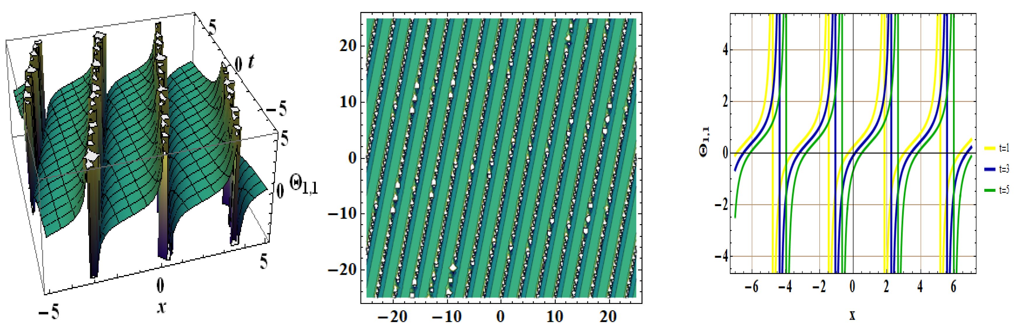
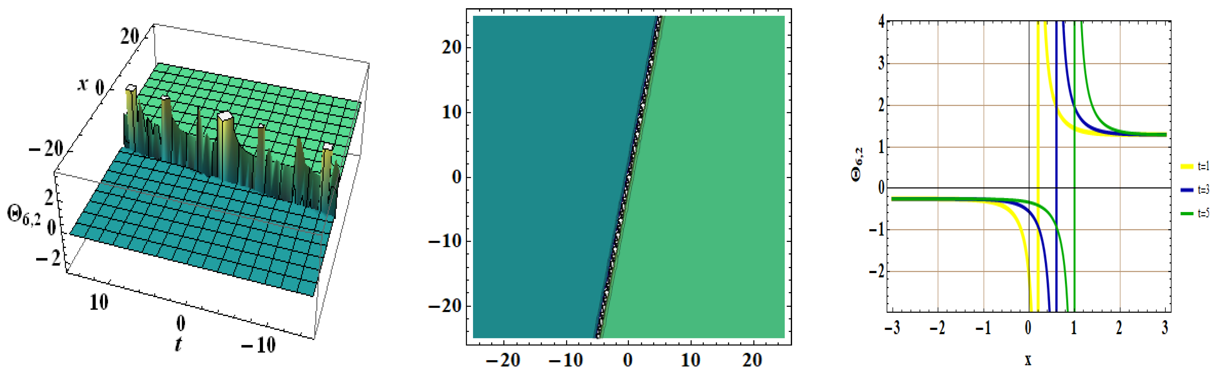
4. Graphical Illustration

The outcomes of the suggested model are visually presented in this section. Through the application of the new auxiliary equation technique, diverse soliton structures have been generated by varying the parameters for each result. The acquired data are depicted through three-dimensional, two-dimensional, and contour plots. Periodic, kink, and singular solitons have been documented for Θ 1 , 1 ( x , t ) , Θ 2 , 2 ( x , t ) , and Θ 6 , 2 ( x , t ) , respectively. The outcomes acquired from the experiments are exhibited in Figure 1, Figure 2 and Figure 3.
Figure 1 illustrates the identification of the periodic solitons solution for Θ 1 , 1 ( x , t ) , corresponding to the parameters ϱ = 2 , α = 1 , λ = 0.1 , and μ = 0.2 . Kink solitons are examined in Figure 2 for Θ 2 , 2 ( x , t ) , exploring various parameter values such as ϱ = 2 , α = 1.3 , λ = 0.25 , and μ = 0.2 . Additionally, Figure 3 presents the singular solitons solution for Θ 6 , 2 ( x , t ) , with the selected parameters ϱ = 3 , α = 0.05 , λ = 0.05 , and μ = 0.2 . The kink solitons represent a noteworthy class that is capable of traversing nonlinear media, showcasing the advanced effects arising from dispersion and nonlinearity. Within the realm of fiber optics, a kink soliton refers to a shock front traversing the dispersive medium without undergoing distortion. Furthermore, each of these outcomes has the ability to maintain its form and velocity when traversing long distances and holds substantial importance in applied scientific domains.

5. Dynamics of the Investigating Model

The current section is used to depict the dynamical nature of the discussed model. For this, we will consider Equation (14) to discuss the behavior of bifurcation [34], chaotic dynamics, and multistability analysis through phase portraits [35].

5.1. Bifurcation Analysis

From Equation (14), we obtain the following planar dynamical system:
d Θ d ρ = Y , d Y d ρ = κ 1 Y + κ 2 Θ κ 3 Θ 3 ,
where κ 1 = ω 2 μ ω 1 , κ 2 = 1 ω 1 , and κ 3 = 1 3 μ ω 1 . The above system has the integral as follows:
L ( Θ , Y ) = ( 1 κ 1 ) 2 Y 2 κ 2 Θ 2 2 + κ 3 Θ 4 4 = l ,
where l is the real parameter. System (32) has the following fixed points on the Θ -axis.
N 1 = ( 0 , 0 ) , N 2 = ( κ 2 κ 3 , 0 ) , N 3 = ( κ 2 κ 3 , 0 ) .
Furthermore, the Jacobian of (32) is:
J ( Θ , Y ) = 0 1 κ 2 3 κ 3 Θ 2 κ 1
= κ 2 + 3 κ 3 Θ 2 ,
Thus ( Θ , Y ) is a saddle point for J ( Θ , Y ) < 0 , a center for J ( Θ , Y ) > 0 , and a cusp if J ( Θ , Y ) = 0 .
In order to examine the nature of system (32) at critical points, the following outcomes are observed.
  • Case 1: Let κ 2 > 0 and κ 3 > 0 .
For κ 2 = 1 , κ 3 = 1 , ω 1 = 1 , and μ = 0.3 , system (32) exhibits three fixed points: N 1 = ( 0 , 0 ) , N 2 = ( 1 , 0 ) , and N 3 = ( 1 , 0 ) . In this case, N 1 is the saddle point and N 2 , N 3 are central points. Additionally, the impact of κ 1 Y has been discussed by taking different values of κ 1 . The phase plots are displayed in Figure 4.
  • Case 2: Let κ 2 < 0 and κ 3 < 0 .
For κ 2 = 1 , κ 3 = 1 , ω 1 = 1 , and μ = 0.3 , the system (32) exhibits three fixed points: N 1 = ( 0 , 0 ) , N 2 = ( 1 , 0 ) , and N 3 = ( 1 , 0 ) . In this case, N 1 is the center and N 2 , N 3 are saddle points. Additionally, the impact of κ 1 Y had been discussed by taking different values of κ 1 . The phase plots are displayed in Figure 5.

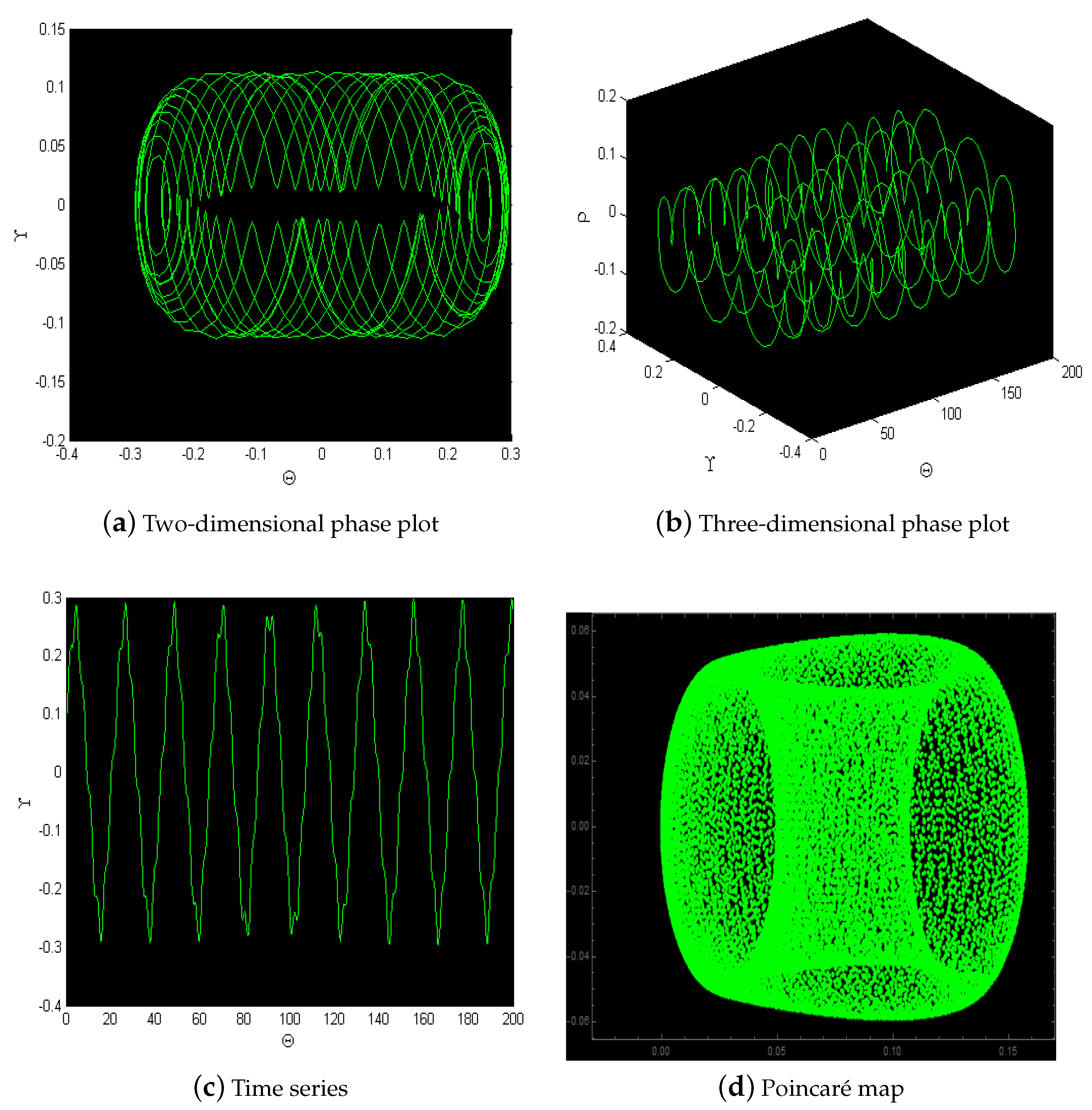
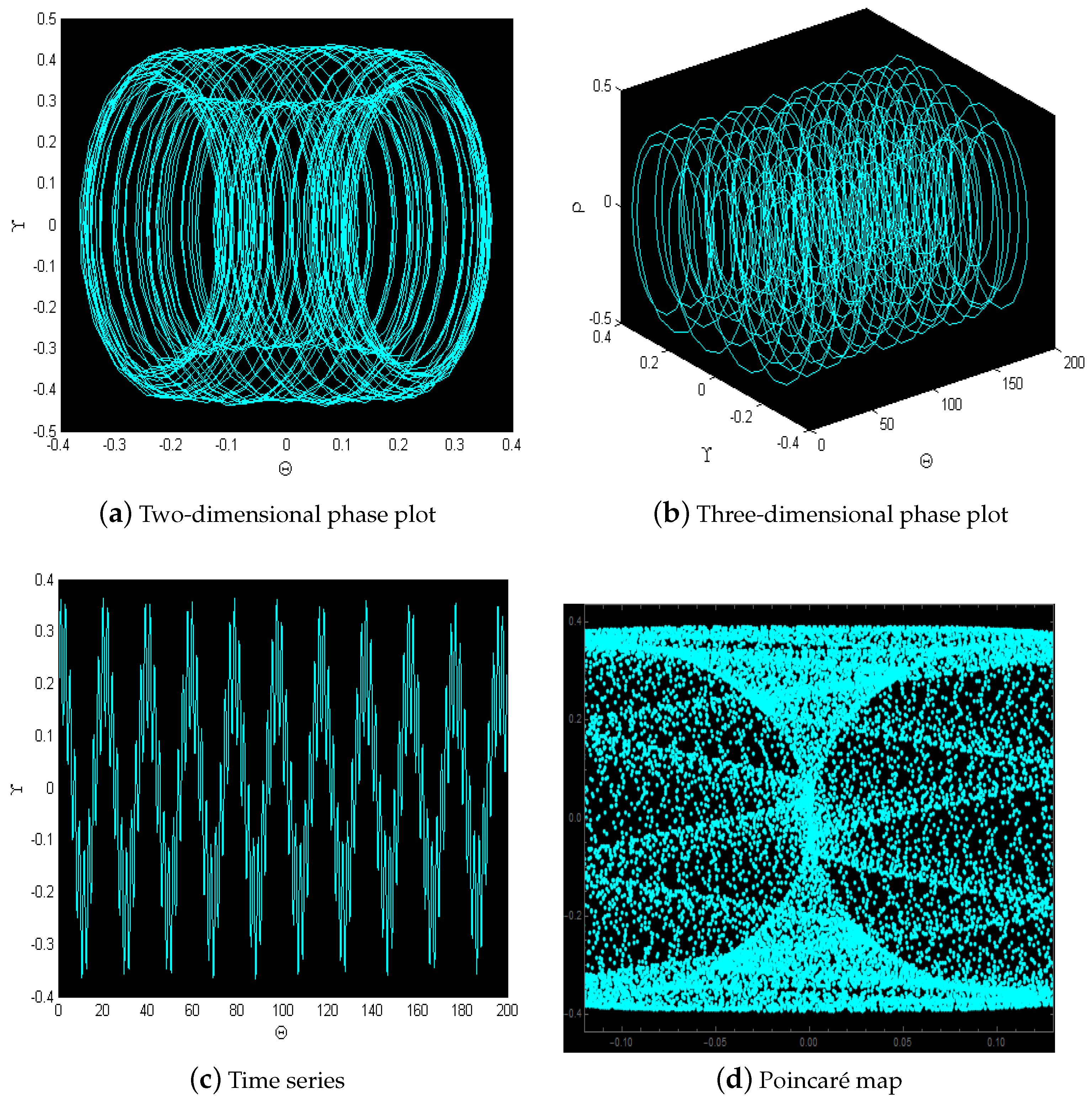
5.2. Behavior of Chaotic Motion

This section examines the nature of quasi-periodic and chaotic dynamics of considered model (3). For this, we incorporate a periodic force into the system (32). Hence, the modified form of the system (32) is:
d Θ d ρ = Y , d Y d ρ = κ 1 Y + κ 2 Θ κ 3 Θ 3 + δ 0 cos ( G ) , d G d ρ = υ .
The aforementioned system is autonomous with G = υ ρ . In the system (34), the external perturbed force consists of two elements, denoted as δ 0 and υ . Here, δ 0 and υ indicate the amplitude and frequency, respectively, of the perturbed term. An unpredictable and random behavior can be observed by adding an eternal force to the planar system. In our work, we have analyzed this phenomenon within a system (32) that demonstrates a chaotic nature, characterized by trajectories diverging from regular patterns and displaying randomness with time. We have investigated the chaotic dynamics of the system (34) using various tools, such as phase plots, time plots, and Poincaré maps. In order to examine the behavior, we will evaluate the influence of the parameters δ 0 and υ .
In Figure 6, the three-dimensional and two-dimensional profiles, time plot, and Poincaré map are shown for the parametric values κ 1 = 0 , κ 2 = 0.02 , κ 3 = 2 , δ 0 = 0.1 , and υ = 2 . It is noted that system (34) is quasi-periodic. In Figure 7, by increasing the amplitude and frequency as δ 0 = 1.1 and υ = 3 while the other parameters remain the same as in the last case, system (34) exhibits irregular patterns. It is evident that the disturbed system demonstrates a chaotic nature under these parameter values. Additionally, the Poincaré map shows numerous scattered points, providing further confirmation of the chaotic nature of the system.

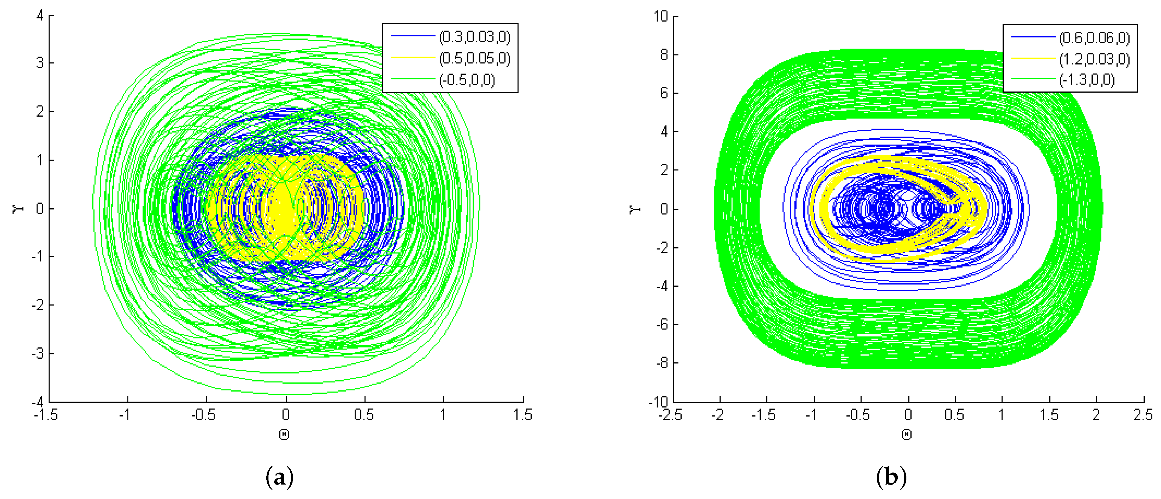
5.3. Multistability Analysis

When a perturbation is introduced to the planar system, it can demonstrate multistability, implying the presence of several possible dynamic behaviors. These behaviors manifest for the same parameter values but distinct initial circumstances. This spectrum of behaviors encompasses chaos, quasi-periodicity, and periodicity, all of which may emerge within the system under varying conditions. In Figure 8, we conducted an analysis of multistability concerning the disturbed system (34) under diverse initial circumstances. Our observations indicate a pronounced sensitivity of system (34) to the initial conditions that result in a chaotic nature.

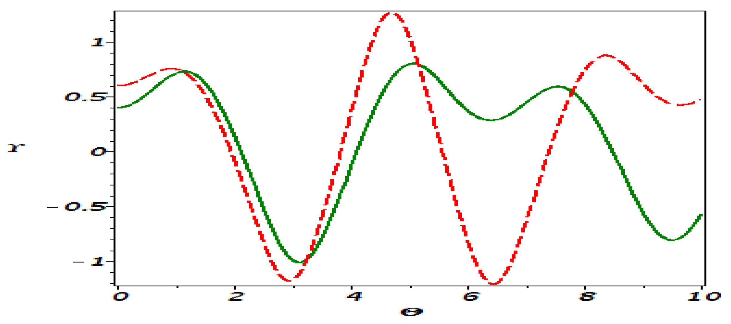
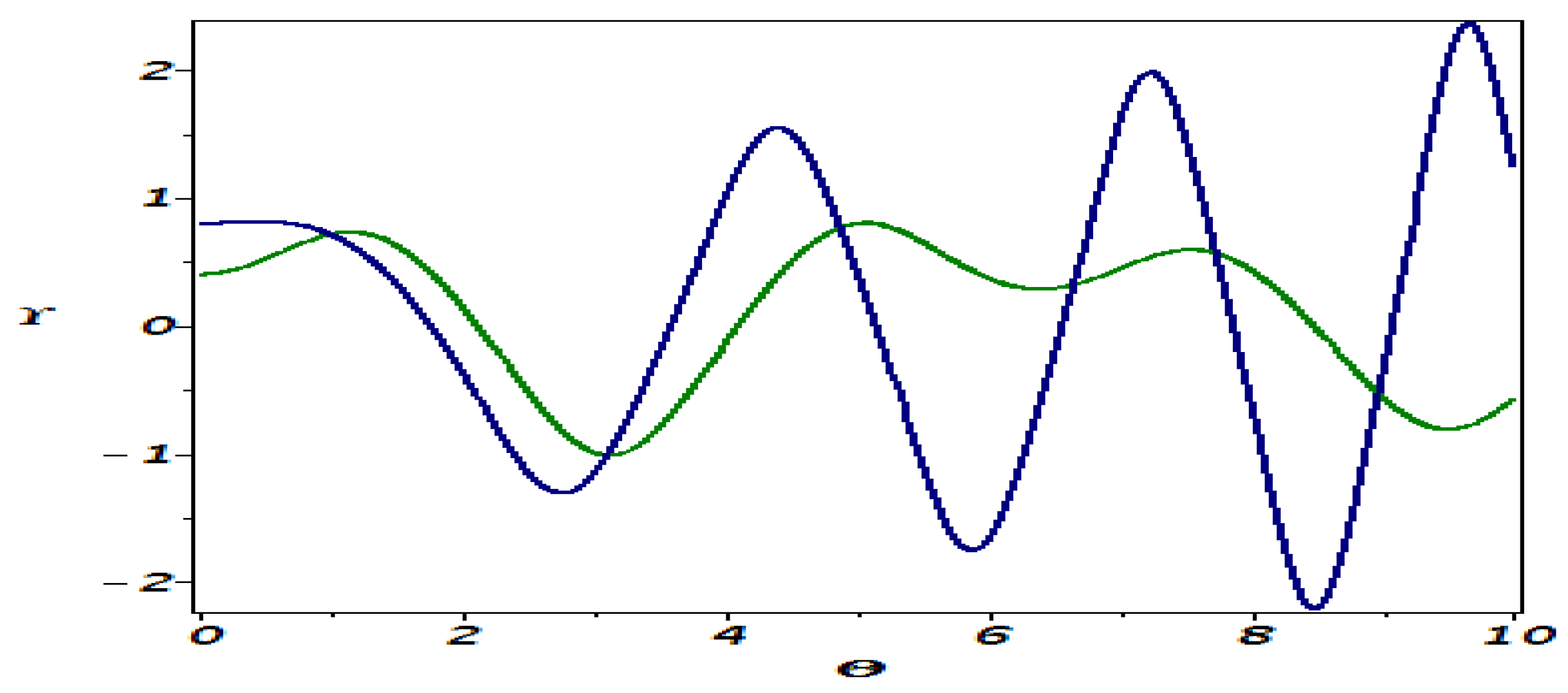
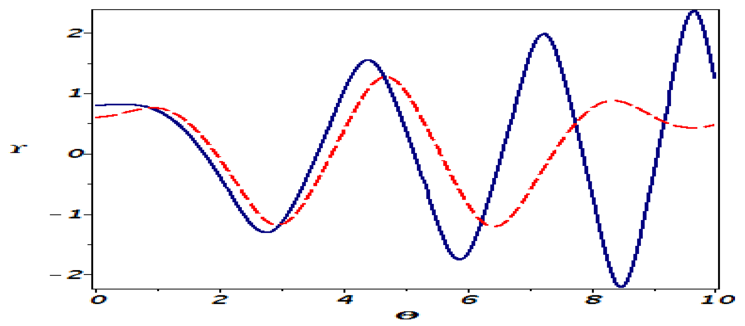
6. Sensitivity Analysis

In this segment, our motivation was to analyze the sensitivity of the system (32). To achieve this, we took into account three distinct initial conditions: ( Θ , Y ) = ( 0.4 , 0 ) in solid green, ( Θ , Y ) = ( 0.6 , 0 ) in red (dashed), and ( Θ , Y ) = ( 0.8 , 0 ) in solid blue. In Figure 9, two solutions are depicted: ( Θ , Y ) = ( 0.4 , 0 ) in green (solid) and ( Θ , Y ) = ( 0.6 , 0 ) in red (dashed). In Figure 10, two solutions are presented: ( Θ , Y ) = ( 0.4 , 0 ) in green (solid) and ( Θ , Y ) = ( 0.8 , 0 ) in blue (solid). In Figure 11, two solutions are displayed: ( Θ , Y ) = ( 0.6 , 0 ) in red (dashed) and ( Θ , Y ) = ( 0.8 , 0 ) in solid blue. A comparison was conducted using various initial values, specifically (0.4, 0), (0.6, 0), and (0.8, 0), as depicted in Figure 12. The outcomes distinctly indicate that minor differences in the initial values significantly influence the final outcome. Hence, it can be deduced that the examined model has a sensitive nature.

7. Concluding Remarks

In this work, we successfully investigated the modified Oskolkov equation, which elucidates the behavior of the incompressible viscoelastic Kelvin–Voigt fluid. Through our analysis, we examined this equation from multiple perspectives, including the Lie symmetry technique, bifurcation analysis, and chaotic behaviors, as well as the sensitive nature of the considered model. First of all, we identified the Lie symmetries of the equation and, utilizing similarity reduction, we changed the partial differential equation into an ordinary differential equation. Solving the obtained ordinary equation with the assistance of the new auxiliary technique, we successfully derived soliton solutions, which are visually depicted in Figure 1, Figure 2 and Figure 3. Furthermore, by performing some calculations, we derived a second-order ordinary equation, yielding a system of first-order DEs (32).
By subjecting the considered model to a bifurcation analysis, we have comprehensively explored its dynamic nature at critical points. This culminated in the depiction of phase portraits, visually represented in Figure 4 and Figure 5. Furthermore, we introduced an external periodic force into the dynamical system, subsequently employing a range of tools to identify chaotic behavior. The utilization of phase plots, Poincaré maps, time plots, and multistability analysis has effectively revealed the presence of quasi-periodic and chaotic dynamics within the disturbed system. These findings are depicted in Figure 6, Figure 7 and Figure 8. In addition, our investigation has highlighted the system’s sensitivity to the initial conditions. Remarkably, even minor adjustments in the initial values lead to considerable variations in the system’s behavior. In conclusion, the outcomes of this study are not only captivating but also underscore the efficacy of the proposed methodologies in assessing soliton dynamics and phase patterns across diverse nonlinear models.

Author Contributions

Conceptualization, M.B.R.; Methodology, M.B.R. and S.S.K.; Software, J.M.; Validation, A.J. and J.M.; Investigation, A.J. and S.S.K.; Resources, J.M.; Data curation, J.M.; Writing—original draft, S.S.K.; Writing—review & editing, M.B.R. and A.J.; Visualization, S.S.K.; Supervision, M.B.R.; Funding acquisition, J.M. All authors have read and agreed to the published version of the manuscript.

Funding

This work was supported by the Ministry of Education, Youth and Sports of the Czech Republic through the e-INFRA CZ (ID:90254).

Data Availability Statement

The data presented in this study are available in article.

Conflicts of Interest

The authors declare no conflict of interest.

References

  1. Zobeiry, N.; Humfeld, K.D. A physics-informed machine learning approach for solving heat transfer equation in advanced manufacturing and engineering applications. Eng. Appl. Artif. Intell. 2021, 101, 104232. [Google Scholar] [CrossRef]
  2. Bruzzone, O.A.; Perri, D.V.; Easdale, M.H. Vegetation responses to variations in climate: A combined ordinary differential equation and sequential Monte Carlo estimation approach. Ecol. Inform. 2023, 73, 101913. [Google Scholar] [CrossRef]
  3. Raza, N.; Ullah, M.A. A comparative study of heat transfer analysis of fractional Maxwell fluid by using Caputo and Caputo–Fabrizio derivatives. Can. J. Phys. 2020, 98, 89–101. [Google Scholar] [CrossRef]
  4. Jornet, M. Modeling of Allee effect in biofilm formation via the stochastic bistable Allen–Cahn partial differential equation. Stoch. Anal. Appl. 2021, 39, 22–32. [Google Scholar] [CrossRef]
  5. Sgura, I.; Lawless, A.S.; Bozzini, B. Parameter estimation for a morphochemical reaction-diffusion model of electrochemical pattern formation. Inverse Probl. Sci. Eng. 2019, 27, 618–647. [Google Scholar] [CrossRef]
  6. Zhang, R.F.; Li, M.C. Bilinear residual network method for solving the exactly explicit solutions of nonlinear evolution equations. Nonlinear Dyn. 2022, 108, 521–531. [Google Scholar] [CrossRef]
  7. Pandir, Y.; Ekin, A. New solitary wave solutions of the Korteweg-de Vries (KdV) equation by new version of the trial equation method. Electron. J. Appl. Math. 2023, 1, 101–113. [Google Scholar] [CrossRef]
  8. Cherniha, R. Comments on the paper “Exact solutions of nonlinear diffusion-convection-reaction equation: A Lie symmetry approach”. Commun. Nonlinear Sci. Numer. Simul. 2021, 102, 105922. [Google Scholar] [CrossRef]
  9. Yin, Y.H.; Lü, X.; Ma, W.X. Bäcklund transformation, exact solutions and diverse interaction phenomena to a (3 + 1)-dimensional nonlinear evolution equation. Nonlinear Dyn. 2022, 108, 4181–4194. [Google Scholar] [CrossRef]
  10. Mohammed, W.W.; Albalahi, A.M.; Albadrani, S.; Aly, E.S.; Sidaoui, R.; Matouk, A.E. The analytical solutions of the stochastic fractional Kuramoto–Sivashinsky equation by using the Riccati equation method. Math. Probl. Eng. 2022, 2022, 1–8. [Google Scholar] [CrossRef]
  11. Shah, R.; Alkhezi, Y.; Alhamad, K. An Analytical Approach to Solve the Fractional Benney Equation Using the q-Homotopy Analysis Transform Method. Symmetry 2023, 15, 669. [Google Scholar] [CrossRef]
  12. Kazmi, S.S.; Jhangeer, A.; Raza, N.; Alrebdi, H.I.; Abdel-Aty, A.H.; Eleuch, H. The Analysis of Bifurcation, Quasi-Periodic and Solitons Patterns to the New Form of the Generalized q-Deformed Sinh-Gordon Equation. Symmetry 2023, 15, 1324. [Google Scholar] [CrossRef]
  13. Liu, Y.; Peng, L. Some novel physical structures of a (2 + 1)-dimensional variable-coefficient Korteweg–de Vries system. Chaos Solitons Fractals 2023, 171, 113430. [Google Scholar] [CrossRef]
  14. Ma, Y.L.; Wazwaz, A.M.; Li, B.Q. Novel bifurcation solitons for an extended Kadomtsev–Petviashvili equation in fluids. Phys. Lett. A 2021, 413, 127585. [Google Scholar] [CrossRef]
  15. Zhang, W.X.; Liu, Y. Integrability and multisoliton solutions of the reverse space and/or time nonlocal Fokas–Lenells equation. Nonlinear Dyn. 2022, 108, 2531–2549. [Google Scholar] [CrossRef]
  16. Gözükizil, Ö.F.; Akçagil, S. The tanh-coth method for some nonlinear pseudoparabolic equations with exact solutions. Adv. Differ. Equations 2013, 2013, 1–18. [Google Scholar] [CrossRef]
  17. Roshid, M.M.; Roshid, H.O. Exact and explicit traveling wave solutions to two nonlinear evolution equations which describe incompressible viscoelastic Kelvin-Voigt fluid. Heliyon 2018, 4. [Google Scholar] [CrossRef] [PubMed]
  18. Karakoc, S.B.G.; Bhowmik, S.K.; Sucu, D.Y. A Novel Scheme Based on Collocation Finite Element Method to Generalised Oskolkov Equation. J. Sci. Arts 2021, 21, 895–908. [Google Scholar] [CrossRef]
  19. Ghanbari, B. New analytical solutions for the oskolkov-type equations in fluid dynamics via a modified methodology. Results Phys. 2021, 28, 104610. [Google Scholar] [CrossRef]
  20. Kaplan, M.; Butt, A.R.; Thabet, H.; Akbulut, A.; Raza, N.; Kumar, D. An effective computational approach and sensitivity analysis to pseudo-parabolic-type equations. Waves Random Complex Media 2021, 1–15. [Google Scholar] [CrossRef]
  21. Uddin, S.; Karim, S.; Alshammari, F.S.; Roshid, H.O.; Noor, N.F.M.; Hoque, F.; Nadeem, M.; Akgül, A. Bifurcation analysis of travelling waves and multi-rogue wave solutions for a nonlinear pseudo-parabolic model of visco-elastic Kelvin-Voigt fluid. Math. Probl. Eng. 2022, 2022, 8227124. [Google Scholar] [CrossRef]
  22. Roshid, M.M.; Bairagi, T.; Rahman, M.M. Lump, interaction of lump and kink and solitonic solution of nonlinear evolution equation which describe incompressible viscoelastic Kelvin–Voigt fluid. Partial. Differ. Equations Appl. Math. 2022, 5, 100354. [Google Scholar] [CrossRef]
  23. Akinfe, K.T. A reliable analytic technique for the modified prototypical Kelvin–Voigt viscoelastic fluid model by means of the hyperbolic tangent function. Partial. Differ. Equations Appl. Math. 2023, 7, 100523. [Google Scholar] [CrossRef]
  24. Hussain, A.; Usman, M.; Al-Sinan, B.R.; Osman, W.M.; Ibrahim, T.F. Symmetry analysis and closed-form invariant solutions of the nonlinear wave equations in elasticity using optimal system of Lie subalgebra. Chin. J. Phys. 2023, 83, 1–13. [Google Scholar] [CrossRef]
  25. Almusawa, H.; Jhangeer, A. Nonlinear self-adjointness, conserved quantities and Lie symmetry of dust size distribution on a shock wave in quantum dusty plasma. Commun. Nonlinear Sci. Numer. Simul. 2022, 114, 106660. [Google Scholar] [CrossRef]
  26. Rahman, R.U.; Al-Maaitah, A.F.; Qousini, M.; Az-Zo’bi, E.A.; Eldin, S.M.; Abuzar, M. New soliton solutions and modulation instability analysis of fractional Huxley equation. Results Phys. 2023, 44, 106163. [Google Scholar] [CrossRef]
  27. Alrebdi, H.I.; Rafiq, M.H.; Fatima, N.; Raza, N.; Rafiq, M.N.; Alshahrani, B.; Abdel-Aty, A.H. Soliton structures and dynamical behaviors for the integrable system of Drinfel’d–Sokolov–Wilson equations in dispersive media. Results Phys. 2023, 46, 106269. [Google Scholar] [CrossRef]
  28. Raza, N.; Kazmi, S.S. Qualitative analysis and stationary optical patterns of nonlinear Schrödinger equation including nonlinear chromatic dispersion. Opt. Quantum Electron. 2023, 55, 718. [Google Scholar] [CrossRef]
  29. Talafha, A.M.; Jhangeer, A.; Kazmi, S.S. Dynamical analysis of (4 + 1)-dimensional Davey Srewartson Kadomtsev Petviashvili equation by employing Lie symmetry approach. Ain Shams Eng. J. 2023, 14, 102537. [Google Scholar] [CrossRef]
  30. Matouk, A.E.; Lahcene, B. Chaotic dynamics in some fractional predator–prey models via a new Caputo operator based on the generalised Gamma function. Chaos Solitons Fractals 2023, 166, 112946. [Google Scholar] [CrossRef]
  31. Rafiq, M.H.; Jannat, N.; Rafiq, M.N. Sensitivity analysis and analytical study of the three-component coupled NLS-type equations in fiber optics. Opt. Quantum Electron. 2023, 55, 637. [Google Scholar] [CrossRef]
  32. Olver, P.J. Applications of Lie Groups to Differential Equations; Springer Science and Business Media: Berlin/Heidelberg, Germany, 1993; Volume 107. [Google Scholar]
  33. Liu, H.; Lie, J.L. symmetry analysis and exact solutions for the short pulse equation. Nonlinear Anal. Theory Methods Appl. 2009, 71, 2126–2133. [Google Scholar] [CrossRef]
  34. Crawford, J.D. Introduction to bifurcation theory. Rev. Mod. Phys. 1991, 63, 991. [Google Scholar] [CrossRef]
  35. Strogatz, S.H. Nonlinear Dynamics and Chaos with Student Solutions Manual: With Applications to Physics, Biology, Chemistry, and Engineering; CRC Press: Boca Raton, FL, USA, 2018. [Google Scholar]
Figure 1. Three-dimensional, two-dimensional, and contour plots for Θ 1 , 1 ( x , t ) by letting ϱ = 2 , α = 1 , λ = 0.1 , and μ = 0.2 .
Symmetry 15 02171 g001
Figure 2. Three-dimensional, two-dimensional, and contour plots for Θ 2 , 2 ( x , t ) by letting ϱ = 2 , α = 1.3 , λ = 0.25 , and μ = 0.2 .
Symmetry 15 02171 g002
Figure 3. Three-dimensional, two-dimensional, and contour plots for Θ 6 , 2 ( x , t ) by letting ϱ = 3 , α = 0.05 , λ = 0.05 , and μ = 0.2 .
Symmetry 15 02171 g003
Figure 4. Phase plots of bifurcation at critical points of the system (32). (a) Impact of the term κ 1 Y on the planar system (32), taking κ 1 = 0.8 , κ 2 > 0 , and κ 3 > 0 . (b) Impact of the term κ 1 Y on the planar system (32), taking κ 1 = 0.4 , κ 2 > 0 , and κ 3 > 0 . (c) Impact of the term κ 1 Y on the planar system (32), taking κ 1 = 0.1 , κ 2 > 0 , and κ 3 > 0 . (d) Impact of the term κ 1 Y on the planar system (32), taking κ 1 = 0 , κ 2 > 0 , and κ 3 > 0 .
Symmetry 15 02171 g004
Figure 5. Phase plots of bifurcation at critical points of the system (32). (a) Impact of the term κ 1 Y on the planar system (32), taking κ 1 = 0.8 , κ 2 < 0 , and κ 3 < 0 . (b) Impact of the term κ 1 Y on the planar system (32), taking κ 1 = 0.4 , κ 2 < 0 , and κ 3 < 0 . (c) Impact of the term κ 1 Y on the planar system (32), taking κ 1 = 0.1 , κ 2 < 0 , and κ 3 < 0 . (d) Impact of the term κ 1 Y on the planar system (32), taking κ 1 = 0 , κ 2 < 0 , and κ 3 < 0 .
Symmetry 15 02171 g005
Figure 6. For κ 1 = 0 , κ 2 = 0.02 , κ 3 = 2 , δ 0 = 0.1 , and υ = 2 , system (34) is presented by utilizing various tools for the detection of chaotic behavior.
Symmetry 15 02171 g006
Figure 7. For κ 1 = 0 , κ 2 = 0.02 , κ 3 = 2 , δ 0 = 1.1 , and υ = 3 , system (34) is presented by utilizing various tools for the detection of chaotic behavior.
Symmetry 15 02171 g007
Figure 8. Identification of chaos for the system (34) using multistability analysis with κ 1 = 0 , κ 2 = 0.02 , κ 3 = 2 , δ 0 = 1.1 , and υ = 3 . (a) Multistability analysis under distinct initial conditions: blue (0.3, 0.03, 0), yellow (0.5, 0.05, 0), and green (−0.5, 0, 0). (b) Multistability analysis under distinct initial conditions: blue (0.6, 0.06, 0), yellow (1.2, 0.03, 0), and green (−1.3, 0, 0).
Symmetry 15 02171 g008
Figure 9. Sensitivity analysis of the model for initial values ( Y , Θ ) = ( 0.4 , 0 ) in green (solid) and ( Θ , Y ) = ( 0.6 , 0 ) in red (dashed).
Symmetry 15 02171 g009
Figure 10. Sensitivity analysis of the model for initial values ( Θ , Y ) = ( 0.4 , 0 ) in green (solid) and ( Θ , Y ) = ( 0.8 , 0 ) in blue (solid).
Symmetry 15 02171 g010
Figure 11. Sensitivity analysis of the model for initial values ( Θ , Y ) = ( 0.6 , 0 ) in red (dashed) and ( Θ , Y ) = ( 0.8 , 0 ) in blue (solid).
Symmetry 15 02171 g011
Figure 12. Sensitivity analysis of the model for initial values ( Θ , Y ) = ( 0.4 , 0 ) in green (solid), ( Θ , Y ) = ( 0.6 , 0 ) in red (dashed), and ( Θ , Y ) = ( 0.8 , 0 ) in blue (solid).
Symmetry 15 02171 g012
Disclaimer/Publisher’s Note: The statements, opinions and data contained in all publications are solely those of the individual author(s) and contributor(s) and not of MDPI and/or the editor(s). MDPI and/or the editor(s) disclaim responsibility for any injury to people or property resulting from any ideas, methods, instructions or products referred to in the content.

