1. Introduction
With the growth of the petrochemical sector, the issue of petrochemical storage tank wall maintenance has become a focal point of businesses. At the moment, manual labor technology is still widely utilized both at home and abroad; not only is manual work efficiency low and pricey, but these duties are also notorious for their dangerous and difficult working environments [
1,
2,
3,
4,
5]. The creation of a dependable wall-climbing robot has become a hot topic in tank maintenance, given the requirement to move with high precision over curved and uneven walls, which places growing demands on performance. Surface adaptation and high-precision trajectory tracking, for example, are important technologies in the field of wall-climbing robots and key technologies for meeting industry needs [
6,
7,
8,
9,
10].
The adsorption, movement and trajectory tracking of wall-climbing robots have been extensively studied, and some typical robotic systems have been developed and applied in various fields. The adsorption mechanism is the primary condition for ensuring the motion of the robot on a vertical surface. Wall-climbing robots have different adsorption mechanisms for different working surfaces and motion modes. Numerous studies have revealed the following five adsorption modes: permanent magnet, electromagnetic, negative pressure, adhesive and propulsive adsorption modes [
11,
12,
13,
14,
15,
16,
17]. Navaprakash et al. [
18] designed an adsorption mechanism using the principle of negative pressure adsorption and verified its safe and stable adsorption on a non-magnetic façade through software simulations. Chen et al. [
19] designed a wall-climbing robot that uses a cyclonic suction unit for climbing rough walls and over small obstacles. Demirjian et al. [
20] designed a Caterpillar wall-climbing robot based on bionic principles, using adhesive materials that break the traditional concept of adsorption. Seriani et al. [
21] used wall-climbing robots to adsorb each other on both sides of the wall to achieve safe adsorption and stable movement on non-magnetic walls. Wang et al. optimized the magnetic circuit by finite element analysis method and designed a new type of permanent magnet wheel with the same arrangement of magnetic pole array, which greatly improved the adsorption efficiency of the magnet. Wen [
22] proposed an adjustable variable magnetic adsorption mechanism to realize the stability detection of the robot on the outer wall of the storage tank. Eto et al. [
23] innovatively designed a two-degree-of-freedom (DOF) rotating magnetic attachment mechanism to maintain the optimal adsorption state of the magnet by passive adjustment to achieve safe and stable adsorption on different wall surfaces. Xiao et al. [
24] designed a new steady-state permanent magnet adsorption operation mechanism to complete the stable adsorption on complex façades. Fan et al. [
25] combined electromagnetic and internal force compensation principles to achieve fast and controlled adsorption and separation of wall-climbing robots.
Many research institutions have developed a large number of wall-climbing robots for industrial applications based on the above adsorption mechanisms, combined with moving mechanisms and detection methods [
26,
27,
28,
29,
30]. Jie Gu et al. [
31] of Nanjing University of Aeronautics and Astronautics proposed a wall-climbing robot with foot suction cups, combining the flexibility of suction cups and foot motion characteristics to achieve adaptive surfaces, but this solution resulted in a less flexible robot with insufficient load capacity. Liu Y et al. [
32] developed a dry-bonded frame multi-legged wall-climbing robot, in which each foot of the robot was adsorbed by adhesion to the wall. The robot moved by alternately lifting and lowering the inner frame as well as the four feet of the outer frame, and used the deformation of the four linked rods to adapt to the curvature of the large façade. Although the robot used relatively novel adsorption and movement methods, the adsorption force of this adsorption method decreased over time, and the load capacity was poor. Huang et al. [
33] combined a crawler structure with a magnetic adsorption mechanism to design a crawler robot for ship inspection, which can achieve large area inspection of complex walls. Han x et al. [
34] developed a wall-climbing robot with a flexible skeleton, whereby fixed magnets on the crawler provided sufficient adsorption force to ensure the robot’s surface adaptivity and stability of motion, but the flexibility was not sufficient. Song et al. [
35] proposed an intelligent off-axis robot based on an improved dual heuristic dynamic programming algorithm based on an intelligent discrete trajectory tracking control algorithm for solving the circular trajectory motion of a robot on a vertical wall. Ti-Li et al. [
36] proposed a mobile robot controller with saturation constraints based on the idea of the backpropagation technique and Lassalle’s invariance principle, but did not consider the problem of unknown parameters in the mobile robot system model. However, the existing studies were only applied to trajectory tracking on the ground, and did not take into account the slip factor present upon elevation. In addition, many methods do not take into account the system response delay or the signal transmission hysteresis, greatly limiting the application of these methods.
Many wall-climbing robots have been developed and utilized for petrochemical maintenance. However, current research is generally bottlenecked due to limitations in reliable adsorption, surface adaptation, and detection equipment, and the following three issues need to be addressed: (1) Due to insufficient research on passive and flexible adaptive movement mechanisms, it is difficult for existing wall-climbing robots to move smoothly on curved surfaces with variable morphologies. (2) The permanent magnet adsorption mechanism has low magnetic energy utilization and adsorption capacity due to the limited analysis of the transfer mechanism of the multi-media magnetic circuit. (3) It is difficult to complete path tracking on vertical surfaces due to insufficient consideration of existing trajectory tracking methods.
Based on the aforementioned issues, this study suggests a wall-climbing robot capable of high-precision operation and maintenance on petrochemical storage tank walls. A high-performance permanent magnetic wheel is developed to tackle the problem of safe adsorption, and the wheel’s fast demagnetization construction is designed to make it easier to remove the robot from the wall after inspection. Unlike traditional rigidly connected wall climbing mechanisms, the actuator unit in this paper is flexibly connected to the robot body to form a pseudo-footed robot that can adapt to curved surfaces and move flexibly on the surface of cylindrical storage tanks. In order to improve the trajectory tracking accuracy, a velocity-compensated controller was designed, the stability of the controller was proved by introducing Lyapunov equation, and experiments were conducted on a 5-mm-thick cylindrical tank surface to test the robot’s structure and high-precision trajectory tracking capability. The experiments show that the robot is able to move flexibly and with high precision on different walls, which can replace manual labor to a certain extent and meet the maintenance operation requirements of wall-climbing robots.
The structure of this paper is as follows.
Section 2 proposes a novel wall-climbing robot structure containing a passive adaptive structure, a barrier-crossing structure, and a magnetic wheel adsorption structure.
Section 3 simplifies the wall-climbing robot as a two-wheel differential speed model using virtual wheels.
Section 4 establishes the trajectory tracking model, proposes the positional compensation control strategy, and designs the speed compensation controller.
Section 5 builds the robot experimental platform to verify the efficiency and superiority of the controller.
2. Introduction of Detection Robot
2.1. Robot Structure
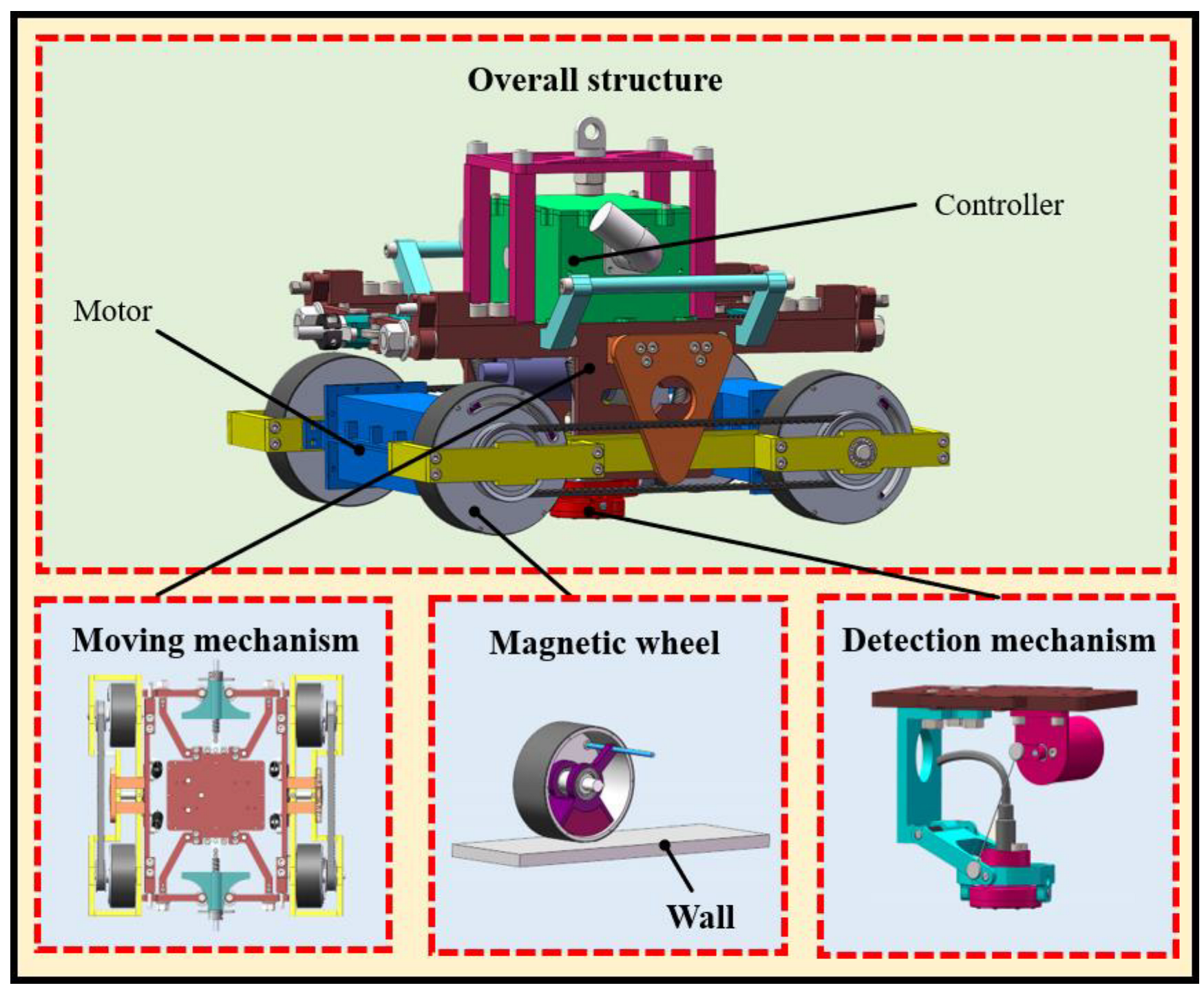
Based on the structural characteristics of petrochemical storage tanks and inspection process analysis, the overall structure of the designed wall-climbing robot for petrochemical storage tank wall inspection is shown in
Figure 1. The robot mainly consists of a surface adaptive motion mechanism, a magnetic adsorption wheel, and a detection mechanism. The two wheels on each side are connected by a drive belt, and two motors are employed, with each driving a single wheel on one side, thus constituting a motor-driven active wheel, while the other wheel is driven by belt drive in order to obtain the same speed and directional motion. The wheels on both sides run separately without interfering with each other, and the motors are arranged symmetrically at the head and tail ends. The overall structure is completely symmetrical, and the differential speed rotation of the wheels on both sides is used to perform vehicle steering. A high-performance magnetic wheel structure with fast demagnetization is also proposed, making it possible to adapt to surfaces with different curvatures by means of coordinating a movement mechanism with multiple degrees of freedom, thus ensuring that the robot has strong adsorption force and is able to quickly perform the demagnetization process, so that the robot can be safely detached from the wall. According to the operation requirements of different inspection modules, a flexible inspection mechanism is designed to combine the pull rope and hook hinge mechanism in order to achieve adaptive vertical alignment of the probe, thus making it adaptable for carrying out different inspection techniques. The inspection robot is able to perform precise movements and the action required for different inspection processes by means of a state control strategy, enabling it to ultimately perform wall inspection tasks.
2.2. Curved Adaptive Floating Mechanism
Since the robots work in environments with façades with different curvatures, safe adsorption and surface adaptation capabilities, as well as the ability to perform high-precision movement while carrying out the work, are the keys to a robot’s successful completion of inspections tasks. To this end, a flexible surface adaptive floating structure is designed, as shown in
Figure 2, through which the robot can reliably adsorb to walls with different façade curvatures in order to meet the requirements of petrochemical storage tank inspection.
The self-adaptive ability of wall-climbing robots, by which they are able to work on surfaces with different curvatures, determines whether or not the robot is stable and safe at work. Conventional wheeled robots work on vertical curved surfaces where, as a result of the integrity of the motion structure, the wheel body is not able to be completely fit to the surface of the wall, meaning that the contact area is insufficient, leading to a reduction in friction that results in slippage and instability, which in turn affect the safety and motion accuracy of the robot. In order to solve the above problems, two types of destabilization for robots during the overcoming and climbing processes are proposed: (1) When the robot lifts a wheel on one side upon encountering an obstacle in the process of overcoming, the other wheel is forced to leave the wall because of the rigid structure of the connection between wheels on the same side, resulting in a reduced contact area and insufficient friction, increasing the risk of skidding or even of falling off. (2) Most of the operating environments of robots are walls with a certain curvature, and when traditional wheeled robots are climbing, to ensure that the body as a whole moves in parallel with the tangent of the wall, the coexistence of the curvature and the rigidity of the frame leads to a certain inclination of the wheels and the wall, which cannot be fit completely to the wall; therefore, the adsorption force between the magnetic wheel and the wall is reduced, which generates instability in the robot and poses a threat to the safety of the robot.
In order to improve the stability of the robot when working at different curvature elevations, while at the same time expanding the fitting area of the robot and the circular steel plate, a surface adaptive floating mechanism was designed. The floating mechanism is mainly comprised of a floating rotary axis, a limiting rod, and a limiting axis. The wheels on the left and right sides are connected by the floating rotary axis to ensure that the wheel carriers on both sides are able to rotate around the axis. When encountering surfaces with different curvatures, the rotation of the floating rotary axis and the micro movement of the limit rod drive the wheel carriers to adapt to the curvature of the surface, so that each wheel adsorbs closely to the wall surface, and the complete fitting movement of the car on the surface can be realized, such that the robot can be safely adsorbed onto walls with different curvatures. The robot uses the adjustability of the cam mechanism to realize the over-the-wall motion, and the cam is pushed to rotate around the swing-back axis by the deformation of the limit buffer spring behind the cam, which is used to prevent the risk of the robot losing stability and falling due to the lifting of the wheels on one side, and to achieve precise adjustment of the stiffness of the robot’s flexible suspension. The drive motor is arranged diagonally, and the synchronous belt is used to transfer the speed, guarantee the driving torque, and simplify the control, so that the robot can complete its work safely and smoothly.
2.3. Magnetic Wheel Design
The magnetic wheel structure’s design is a crucial aspect in determining whether the wall-climbing robot can move safely and stably on the wall. Any movement during the inspection process that causes a change in the magnetic force will lead to an increased risk of the robot breaking away from the wall, so designing a magnetic wheel that is suitable for wall motion and enables the robot to attach to the wall safely and stably is a prerequisite for robot motion. First of all, in the process of designing the magnetic wheel structure, the key to determining the safe and stable movement of the robot on the wall is the adsorption force of the magnetic wheel. When the adsorption force of the magnetic wheel is too great, the robot’s movement is more stable, and the safety factor is high. However, due to the increased adsorption force, the friction between the magnetic wheel and the wall will be too high, and the torque generated by the differential steering and movement of the vehicle will increase significantly, making it difficult for the robot to detach itself from the wall when the inspection work has been completed. When the magnetic wheel adsorption force is too small, the necessary conditions for robot adsorption cannot be met. The above-mentioned problems were combined in order to design a lightweight magnetic wheel with strong adsorption with which the safe and stable attachment of the robot to the wall can be ensured and the torque required for the differential motion of the robot can be reduced, while the demagnetization process after the work is finished can be completed quickly.
In order to improve the utilization rate of the magnet, the overall design used the structural shape of the sector-shaped permanent magnet and combined it with the yoke iron to reduce the overall weight of the wheel, while meeting the magnetic force requirements, and the electromagnetic field analysis software Ansys was used to analyze the influence of the magnet’s structure on the adsorption force of the wheel and to design the shape of the magnet, shown in
Figure 3, thus completing the design of the lightweight wheel. In the process of generating the adsorption force of the magnetic wheel, most of the magnetic induction lines come from the small part of the magnet near the side wall. Therefore, a radially magnetized fan magnet (Nd2Fe14B) was chosen as the excitation source in order to reduce weight and provide a strong adsorption force. The yoke itself does not generate magnetic induction lines, and its high permeability properties in the magnetic circuit can be used to transmit magnetic force in order to reduce the occurrence of magnetic leakage and improve the utilization of the magnet. After completing the wall inspection task, the robot needs to be safely detached from the wall, and the demagnetization process of the magnet wheel is completed.
To achieve the purpose of actively reducing the adsorption force of the magnet wheel, a smaller tangential force can be used to force the magnet to rotate relatively in the adsorption state, thus reducing the adsorption force between the magnet and the wall. Therefore, in order to complete the separation of the wheel from the wall in a stable and safe manner, after the robot has finished its work, a fast demagnetization mechanism is designed using the lever principle, as shown in
Figure 3, which applies a tangential force to the magnet wheel using the demagnetization bar to facilitate the magnet’s rotating around the output axis after the robot has stopped working, thus completing the demagnetization process.
3. Design of the Virtual Wheel
In order to achieve the precise control required for the operation of the wall-climbing robot, the concept of virtual wheels was introduced for the analysis of the robot kinematic model. By streamlining the robot kinematic model and combining the temporal changes in the virtual wheel radius values, the left and right wheel velocities of the robot are compensated accordingly in order to achieve accurate trajectory tracking.
3.1. Concept of the Virtual Wheel
Improving the precision control of the robot’s motion is key to designing the robot, because of the high accuracy required for inspection tasks. Since the robot itself has a four-wheel drive structure and works on a vertical surface, it is difficult to quantify the sliding error generated by these external factors due to the influence of gravity and other factors. In this section, we propose the idea of a virtual wheel to simplify the model by equating the changing distance to a virtual wheel radius, defining the virtual wheel rotation center at the center of the wheel frame, and simplifying the robot model into a two-wheel differential speed model. The change in the virtual wheel radius can also be equated to plane motion, and then the simplified kinematic model can be used to achieve accurate control of the robot’s surface motion.
In
Figure 4, the virtual wheel states of the unilateral wheel frame of the robot under walls with three different curvatures are shown. The overall model of the robot is simplified by using the virtual wheel defined here, and the simplified model is shown in
Figure 5.
3.2. Solution of the Virtual Wheel
In order to achieve more accurate control of robot posture and more efficient control of robot pre-travel trajectory for virtual wheel concept proposed in the previous section, the global coordinate system is established by XOYOZ, in order to accurately describe the current position of the robot and the coordinates of each wheel center, and to calculate the radii of the left and right virtual wheels at this moment on the basis of the parameters of the current position of the robot.
First, a complete global coordinate system is established to describe the coordinates of each wheel of the robot, and then the robot trajectory equation is determined on the basis of the robot’s heading angle, and the virtual wheel radius is calculated from the position of each wheel center in the trajectory equation. This model is built on the premise that there will be no slip and skid under the rigid structure of the robot, and the global coordinate system is established on the basis of the position of the robot and in line with the wall parameters. A schematic diagram of the robot’s position at a heading angle of
is shown in
Figure 6, where the cylindrical sketch is a simplified model of the robot’s working wall. The coordinates of the robot’s unilateral active wheel in the global coordinate system are defined as
; the coordinates of the driven wheel are
; and the virtual wheel coordinates are
. Since the
-axis parameter after the coordinate system conversion is independent of the virtual wheel radius, the change in the
-axis parameter is ignored for the sake of simplicity of operation. Therefore, for
,
,
, a coordinate system transformation is performed as follows, and the new coordinate system is defined as the trajectory coordinate system
:
where
is the rotation matrix and
is the heading angle.
The coordinates after the matrix transformation are shown below.
Regarding the detailed parameters of the virtual wheel radius, two instantaneous momentary attitude diagrams of the robot’s unilateral wheels are established, as shown in
Figure 7, in which the two models are position diagrams at moment
and moment
, respectively, and the elliptical trajectory in which the robot body is in the desired elliptical trajectory when the heading angle is
,
and
indicates the center of the circle of the two solid wheels, respectively. The distance between the center of the virtual wheel circle and the elliptical trajectory at this moment is
. According to
Figure 7, the virtual wheel center is located at the midpoint of the line connecting the two solid wheel centers, and the curvature of the elliptical reference trajectory of the pre-row is relatively flat, due to the small degree of curvature of the actual wall on which the robot is working, and the smooth overall running speed, Therefore, we can make a straight line
perpendicular to the line
, intersecting the elliptical trajectory at the point
. The error of the minimum value of the equation from
to the elliptical trajectory is very small, so the distance
can be regarded as the virtual wheel radius value, and the virtual wheel radius can be taken as
. Therefore,
.
The coordinates of the circle centers of the two solid wheels are
The coordinates of the center of the virtual wheel circle are .
The expected trajectory equation of the robot for a short time at the current heading angle of the position is
where
is the radius of the surface.
Combining the equation of line
with the equation of the elliptical trajectory, the coordinates of point
are
, so the radius of the unilateral virtual wheel is
Similarly, by borrowing the coordinates of each wheel center on the left side, we can find the virtual wheel radius on the other side at that moment .
3.3. Relationship between Virtual Wheel and Solid Wheel
When the robot is in different poses at different times, the radii of its solid and virtual wheels are not equivalent, resulting in unequal velocities, so this section explores the connection between the two velocities in detail.
According to the change in the robot’s heading angle and the working environment as a surface, it can be seen that the robot’s reference trajectory is an elliptical trajectory with a curvature variable with the change in heading angle, and the instantaneous expected trajectory equation for the robot’s heading angle of
in the positional position is
It is assumed that the solid wheel’s linear velocity direction is constantly tangential to the trajectory, whereas the virtual wheel maintains pure rolling contact with the wall, and is subject to no slippage. The active wheel linear speed is , the angular velocity is , the linear speed of the virtual wheel is , the angular velocity is , the linear speed of the driven wheel driven by the main wheel is defined as , and the angular velocity is .
As the robot’s heading angle changes during the working process, the robot’s reference trajectory changes, and thus the radius of the virtual wheels on both sides changes. When the robot moves vertically up the wall, the radius of the virtual wheels is maximized, as . When the robot is moving horizontally on the wall, at this moment, the virtual wheel radius reaches its minimum value, and the value of at this moment is related to the magnitude of the curvature of the wall, Thus, .
Considered from the point of view of speed, within the instantaneous moment , , because the active wheel and the driven wheel are connected with the conveyor belt, there is an unavoidable loss in the speed transfer process, and the driven wheel speed is , it can be seen that the driven wheel speed is in a process that significantly increases and approaches the active wheel speed in a very short time, and there is a very short time error between them. Therefore, it can be seen that there is a small error between the wheel speed of the active wheel and the wheel speed of the driven wheel. In view of the fact that the wheel center of the virtual wheel is defined on the wheel frame, reducing the wheel speed error between the active wheel and the virtual wheel and the loss caused by the conveyor belt, we initially consider that, if the virtual wheel speed is determined by the driven wheel speed, the error will be larger than that determined for the active wheel, and the speed relationship between the active wheel and the virtual wheel can be used directly to reduce speed error.
In the same moment
, the active wheel is determined on the basis of the trajectory course for
, the virtual wheel on the same side can be determined through the distance for
, because the curvature of the robot’s elliptical reference trajectory changes from time to time, so that there is a small error in the size of the distance traveled by both, where an error value of
is proposed, and the relationship between the sizes of the two distances is as follows:
Therefore, there is also a small error between the linear speed of the virtual wheel and the linear speed of the active wheel, and we get
From the perspective of the overall system error, this velocity error is caused by the characteristics of the surface itself and the motion on the robot body surface, and can be considered in conjunction with the angular velocity relationship between the two. Combined with the fact that the robot’s working environment is a vertical surface with a small degree of curvature, the existence of friction between the robot’s active wheel and the wall during motion, as well as the slippage phenomenon within a very short distance, is one of the main reasons for the deviation of the robot motion trajectory. However, since the virtual wheel is a hypothetical object, there is no friction with the wall surface. In addition, in actual operation, the angular velocity of the virtual wheel is always greater than or equal to the angular velocity of the active wheel. Combining the above conclusions, in practice, we can compensate the error between the angular velocity of the virtual wheel and the angular velocity of the solid wheel with the loss of the solid wheel, so as to reduce the speed loss of the solid wheel. Therefore, in summary, the larger angular velocity of the virtual wheel can reduce the velocity friction loss of the active wheel, thus reducing the system error. The angular velocity relationship between the active wheel and the virtual wheel is as follows:
4. Track Tracking
Since the wall-climbing robot is a typical incomplete system and the working environment is a vertical curved surface, it is bound to be affected by gravity as well as friction and other factors, leading to different degrees of slippage when the robot is following the path, while the vector direction of the wheel speed keeps changing on both sides of the robot while the robot is moving on the curved surface, resulting in it being impossible to track the desired route accurately and in a timely fashion, rendering the robot unable to perform an efficient and accurate inspection of the wall. In order to address the above problems, in this chapter, the virtual wheel proposed in the previous section and the velocity relationship between the virtual wheel and the active wheel are combined in order to simplify the four-wheel robot model into a two-wheel differential speed model by means of the virtual wheel, equating the motion of the robot along the surface into planar motion by incorporating the change in the virtual wheel radius, designing a control law using the backstepping method, and calculating the time error compensation for the non-synchronous nature of the system response and feedback duration, in order to achieve a stable convergence of the actual robot trajectory on the target trajectory starting from any initial position, which is thus able to realize the purpose of real-time deflection correction for the robot when in the traveling state, and enables the robot to perform the wall inspection task with high efficiency and high precision.
4.1. Robot Kinematic Model
The robot system model is the basis for studying the robot control algorithm, and in order to better realize high-precision trajectory tracking of the robot, in this chapter, the mathematical model of the system is first established, and the real-time differential equation of positional error is solved using kinematic modeling. The robot systematic error model is shown in
Figure 8. The robot body is simplified to be composed of two driving wheels and the car body by using virtual wheels, where the left and right wheels are the driving wheels.
As shown in
Figure 8, the generalized coordinate vector is defined as
to represent the initial pose of the robot body in a two-dimensional global coordinate system
, and
indicates the reference position of the robot body at the next moment, where
is rotation counterclockwise in the positive direction.
indicates the initial motion state of the robot body and the robot motion state in the reference position is
. As shown in
Figure 8, the motion model of the robot is
In the local coordinate system, the robot’s positional inaccuracy is defined as
According to the geometric relations in
Figure 8, the robot’s positional error within the coordinates can be obtained as [
37]
Taking the time derivative of the above equation and simplifying it yields the differential equation shown below:
4.2. Design of Trajectory Tracking Controller
According to the above kinematic equations, the solution to the trajectory tracking problem of the wall-climbing robot is to control the robot with bounded inputs , make the robot track the reference pose in any initial error state and reference input , with bounded, while satisfying the robot system with any initial tracking error of .
Combining the equation for solid wheel speed and virtual wheel speed presented in
Section 2, the control law as described in Equation (13) was designed [
38,
39]. Let the control parameters
,
,
be bounded, and considering the delay in time feedback, the following control law should satisfy the conditions of no response time error and no time feedback error in the system.
According to the control law described above in Equation (13), the Lyapunov function is designed as shown in Equation (14).
The derivative is obtained by combining the control law
and the error differential equation, as follows:
where the control parameters
,
and
are greater than 0.
Based on the results of the above equation, it can be concluded that this control law causes the robot system to converge asymptotically on the equilibrium point with no response delay; then, the robot is able to automatically track the reference trajectory.
4.3. Time Compensation
In the process of trajectory tracking under the above control law, there is a delay in the system response time, and there is also a delay in the position information feedback of the robot at each moment, leading to a deviation in the error evolution of the motion model, which is positively correlated with the time function. Therefore, from a simple calculation point of view, the overall response time of the system is ignored, and only the errors caused by the time delay of position information output and feedback are compensated. This reduces the position tracking error and allows tracking to be performed as quickly as possible.
The output response moment within the position feedback device is defined as , the moment at which the signal is received and processed from the system controller and fed back into the device is denoted as ; therefore, the amount of time delay is where , is the sampling time, and .
It is assumed that in
time, the robot continues to advance a distance under the initial error model, defining the distance as
. Before that, after assuming the surfaces on which the robot is moving to be expandable planes in conjunction with the virtual wheel concept as described in
Section 3, the paths in the time
can occur in the same plane. Due to the randomness of positional deviation and the difference in the degree of left and right wheel slip, the robot center-of-mass line
at two adjacent moments does not exactly coincide with the actual route
of robot motion. A discrete-time parameter value is introduced here,
, where
, so
The change in attitude declination can be simply defined as .
Therefore, the error model at the moment
is
Then, the new control law can be designed as follows:
Then, by combining the
functionals constructed above and the derivative of the error differential equation, the final result is as follows:
Based on the results of the above equation, it can be concluded that the control law compensates for the robot system for the time feedback error and the overall asymptotic convergence to the equilibrium point can be achieved by automatically tracking the reference trajectory.
Figure 9 presents a block diagram of the trajectory tracking process.
5. Experiment on Prototype Machine
Combining the magnetic wheel and the flexible moving mechanism introduced above, the main target of the robot is to perform the task of inspecting the wall thickness of vertical walls with a certain curvature. The key technical parameters are shown in
Table 1.
In this chapter, the performance of trajectory correction of the wall-climbing robot is discussed, as well as the results of the trajectory tracking test performed to verify the rationality and feasibility of the virtual wheel idea described above and the controller designed on the basis of the virtual wheel. The experimental setup mainly comprised the robot control system and a cylindrical façade.
Figure 10 shows a vertical circular steel plate with a radius of 8 m and a wall thickness of 5 mm for the simulation of a storage tank environment. The wall-climbing robot system includes the robot body, the control box, and the auxiliary equipment. The mobile robot accomplishes autonomous movement by means of the control unit in order to complete the trajectory tracking task of the façade.
A circular arc trajectory tracking experiment was conducted on a vertical arc steel plate to examine the robot’s accuracy when tracking trajectories on curved surfaces. The tracking performance of the robot was analyzed by monitoring the rotational speed of each wheel and the change in the position of the robot’s center of mass during the circular motion of the robot on the curved plate. The robot was controlled to move from vertical upward to horizontal rightward, and the changes in wheel rotational speed and center of mass were detected during this process, with the wheel speed information being obtained by detecting the encoder information of the wheel motor, while the robot position information was obtained using the inertial navigation module mounted on the moving mechanism. The steel plate used in the experiment was unfolded along its circumference to visualize the motion and to plot the center-of-mass variation curve. The trajectory tracking test was carried out without utilizing the compensated control model. First, the robot driving trajectory was set, with the speed output from the original trajectory being taken as the standard value; then, the experimental data were automatically detected and recorded. Specific details of the experimental process and the test data are shown in
Figure 11.
The robot did not lose its stability, and completed the right turning movement from the vertical direction to the horizontal direction in the experiment described above. The left and right wheel rotation speeds were set at 0.18 m/s and 0.09 m/s, respectively; therefore, the expected theoretical turning radius was 0.8 m. The experimental data show that the robot was able to move smoothly to the end of the set trajectory during the motion, but the actual speed fluctuated greatly with respect to the expected speed, resulting in obvious deviations between the robot’s travel trajectory and the expected set trajectory, and thus not meeting the requirements of high-precision operation. In order to reduce the offset error of the robot trajectory, an error compensation controller was added, and the above experiment was conducted again. Specific details regarding the experimental procedure and test data are shown in
Figure 12.
During the experimental process, the robot was also able to complete the trajectory tracking task successfully, and it was obvious from the experimental results that the deviation between the real-time speed of the robot and the expected speed became smaller, converging to the expected speed, and the actual walking trajectory of the robot was close to the predetermined trajectory, while the two sets of test data fluctuated at the weld seam due to the influence of the welding quality and the location of the measurement point. For this reason, the problem of moving accuracy at the weld seam was temporarily ignored. Stable data were able to be collected at other locations, and the test results met the expected target, thus demonstrating improved the robot travel trajectory accuracy and meeting the requirements of most work tasks.
In conclusion, the robot system based on error compensation model control exhibited higher speed accuracy, smaller positional tracking error, and better reference trajectory tracking capability than before, improving the precision operation of wall-climbing robots.
6. Conclusions
In order to address problems related to the poor surface adaptation and low control accuracy of traditional petrochemical tank wall-climbing robots, the high-precision tracking trajectory of the elevation adaptive wall-climbing robot was optimized. To solve the trajectory offset problem caused by signal time lag, a velocity compensation model was proposed to correct the robot’s trajectory using the velocity compensation method of the robot drive wheel, and the position error model was established by simplifying the wall-climbing robot into a two-wheel differential velocity model through the implementation of a virtual wheel. In addition, the trajectory error relationship of the above kinematic controller was determined, the velocity compensation controller was designed using the inverse method, and the multi-feedback closed-loop time lag error compensation controller was designed using the motion state and response time of the previous moment as parameters; thus, the time lag compensation of the virtual wheel velocity was finally obtained, successfully achieving the aim of reducing the trajectory tracking error and ensuring the flexibility and stability of the wheeled robot’s motion on the surface.
The wall-climbing inspection robot was tested on an external wall with a thickness of 5 mm, and its accuracy was compared with that of the pre-compensated model, whereby the amplitude of wheel speed fluctuation was reduced by 9%, trajectory error was reduced by 21%, and the trajectory jitter was also reduced. The experiments showed that the robot could be stably attached to the façade and was able to move with high accuracy on the variable curvature façade, proving that the adaptive mechanism and compensation method were accurate, feasible and effective. The experiments also showed that the robot could be used in environments where the curvature of the petrochemical tank walls varies greatly.


