Abstract
In this paper, the main concepts of interval type-2 (IT2), generalized type-2 (GT2), and interval type-3 (IT3) fuzzy logic systems (FLSs) are mathematically and graphically studied. In representation approaches of fuzzy sets (FSs), the main differences between IT2, GT2, and IT3 fuzzy sets were investigated. For the first time, the simple Matlab Simulink and M-files by illustrative examples and symmetrical FSs are presented for the practical use of IT3-FLSs. The computations were simplified for the practical use of IT3-FLSs. By the use of various examples, such as online identification, offline time series modeling, and a robotic control system, the design of IT3-FLSs is elaborated. The required derivative equations are also presented to design the adaptation laws for the rule parameters easily in other learning schemes. Some simulation examples show that the designed M-files and Simulink work well and result in a good performance.
1. Introduction
Today, various usages of type-1, type-2, and type-3 FLSs are reported in the literature (shorturl.at/asMPS; click here to get access to Matlab codes), such as: clustering [1], control problems [2,3], identification and modeling problems [4], forecasting applications [5], performance evaluation systems [6], image processing [7], among many others.
To promote the efficiency of conventional FLSs, the IT2 and GT2 FLSs have been presented. Up to now, many learning algorithms and optimization techniques have been suggested to make FLSs more applicable. For example, in [8,9], the galactic swarm optimization approach was developed to adjust the rules of IT2-FLSs, and in a noisy robotic application, its efficiency was evaluated. In [10], by using T1 and IT2 fuzzy systems, a classifier was designed for the pulse level, practically implemented, and the better performance of IT2-FLSs in a practical environment was shown. In [11], the slime mold method was used for destining a T2-FLS-based controller, and some comparisons were provided to show the effectiveness of T2-FLSs. A decision-making system was designed in [12] using T2-FLSs, and it was shown that the T2-FLSs led to a good result in terms of sensitivity, flexibility, and stability. In [13], an application of T2-FLSs was investigated in the Internet of Things, and it was verified that T2-FLSs increase the packet transmission ratio and lifetime. In [14], a risk assessment approach was developed to evaluate the renewable energy sources, and the capability of T2-FLSs in large-scale problems was examined.
More recently, type-3 FLSs have been introduced to enhance the uncertainty modeling competency of T2-FLSs. In various applications, the efficiency of T3-FLSs has been examined. The concept of T3-FLSs for the first time was introduced by Ardashir M. Zadeh et al. in [15]. In this paper, it was shown that IT3-FLSs perform better in noisy real-world situations. In [16,17], a control application of T3-FLSs was presented, and the good accuracy of T3-FLSs was shown in a microgrid control problem. Under challenging circumstances such as time-variant and unknowable dynamics, the performance of the T3-FLS-based approach was tested. When compared to traditional management techniques, the recommended methodology performed better in terms of regulation since, unlike the approaches in question, all mathematical dynamics were taken to be unknown. In [2], some concepts of IT3-FLSs were summarized, and the main developments were reviewed. In [18], an IT3-FLS based controller was used to stabilize a 5G telecom, and by experimentally evaluating the superiority of IT3-FLSs in a noisy environment, its performance was confirmed. The suggested T3-FLS-based system is used in 5G base transceiver stations to effectively stabilize full-bridge converters and provide uninterrupted power to associated loads. In [19], another practical application of IT3-FLS was investigated. By an experimental scheme, the accuracy of an IT3-FLS-based controller was studied by applying it to DC converts. Due to their negative impedance requirements, power electronic devices are susceptible to instability while delivering steady power loads. The T3-FLSs are employed to ensure the stability of these devices. The instability problem was resolved by the T3-FLS-based controller, which also controls the output voltage’s reaction.
In [20], a clustering algorithm was designed based on IT3-FLSs, and the better efficiency of the IT3-FLS was proven by various benchmark data. This article presented a design process for Mamdani IT3-FLSs. The deep learning of T3-FLSs was studied in [21]. In this paper, a method for estimating CO2 solubility was introduced. This method was based on a novel deep learning T3-FLS. It was advised that the provided model be optimized using a hybrid learning approach. The purpose of the adaption laws is to fine-tune the rule parameters and membership function centers (MFs). A Kalman filter learns the level of the horizontal slices. The paper in [22] described a method for parameterizing T3-MFs that applies vertical cuts to the differential evolution algorithm’s dynamic parameter adaption and implemented in a T3 Sugeno controller. To enhance the performance of this technology as the generations pass, it was used for dynamic adaption. The best design for a T3-FLS-based controller was taken into consideration in order to evaluate the differential evolution algorithm. The parameterization of the controller’s T3-MFs was performed in this instance. To validate the effectiveness and conduct a comparison research with other papers in the literature, the experimentation was on the basis of distinct noise levels. The prediction ability of T3-FLSs was examined in [5]. This study made a COVID-19 forecast using a mix of a T3-FLS and fractal theory. In this instance, the COVID-19 issue was used to evaluate the time series geometrical complexity level using the fractal dimension. Utilizing the T3-FLS was primarily intended to handle uncertainty in predicting decision-making. A T3-FLS model with fuzzy if–then rules that uses the linear/non-linear dimension values as inputs and produces COVID-19 case predictions makes up the hybrid technique.
The contributions of this paper are as follows:
- A type-3 FLS with simplified computations is presented.
- The fundamental differences between various FLSs were analyzed in both theoretical and numerical approaches.
- A simple Matlab implementation scheme is presented for practical applications.
- A straightforward scheme is presented for designing the T3-FLSs.
- Application of the T3-FLSs in online applications was simplified.
In the remainder of this paper, a general review is given in Section 2. The structure of T3-FLSs and the learning scheme are explained in Section 3 and Section 4. The Simulink and M-file implementations are given in Section 5 and Section 6. Finally, the simulations and conclusions are presented in Section 7 and Section 8.
2. General View
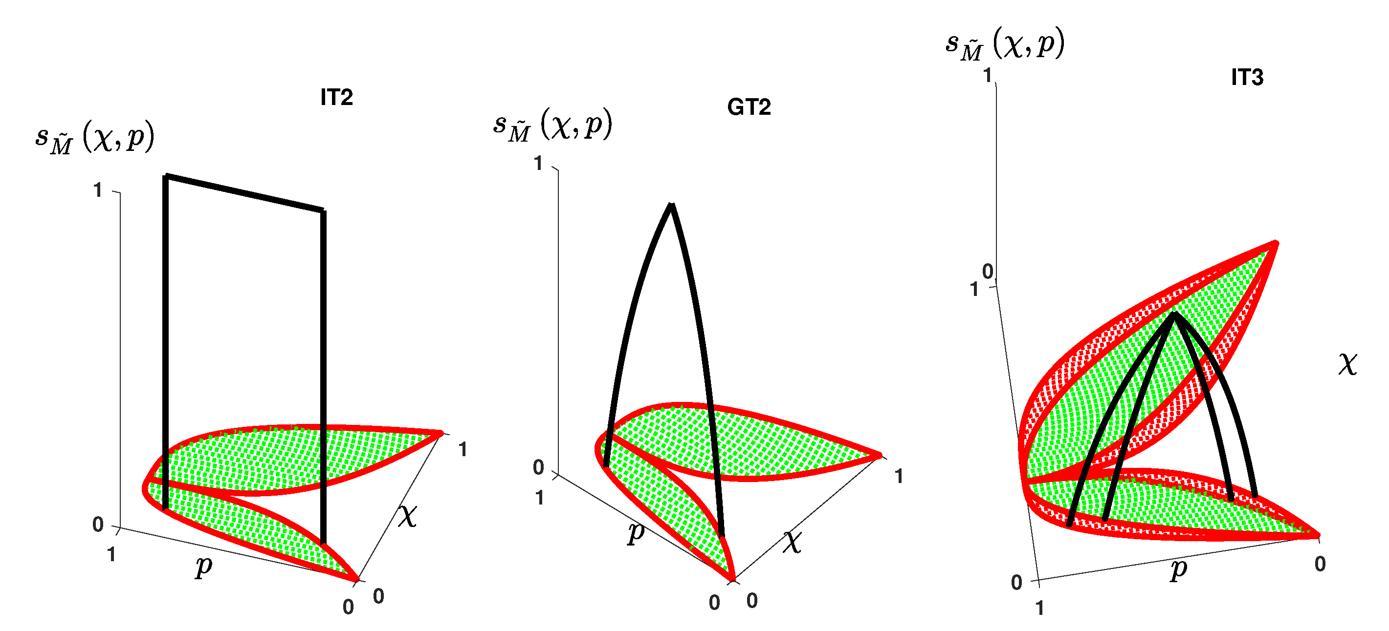
To have a general view of the difference between IT2, GT2, and IT3 fuzzy sets, an example is given in Figure 1. The secondary membership for a IT2-FS is a crisp value; GT2-FS is a type-1 FS, and IT3-FS is a type-2 FS. Then, the IT3-FSs can model a higher level of fuzziness and uncertainties than the IT2-FS and GT2-FSs. Furthermore, in the comparison of GT2-FSs and IT2-FSs, we see that the secondary membership in the GT2-FSs is a fuzzy number; however, in the IT2-FSs, it is a fixed number. Then, GT2-FSs have a better uncertainty modeling capability than IT2-FSs.
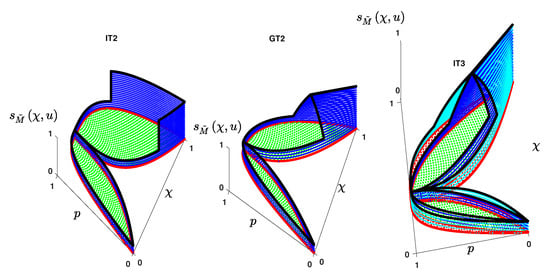
Figure 1.
A general view on IT2, GT2, and IT3 fuzzy sets (some horizontal and vertical slices).
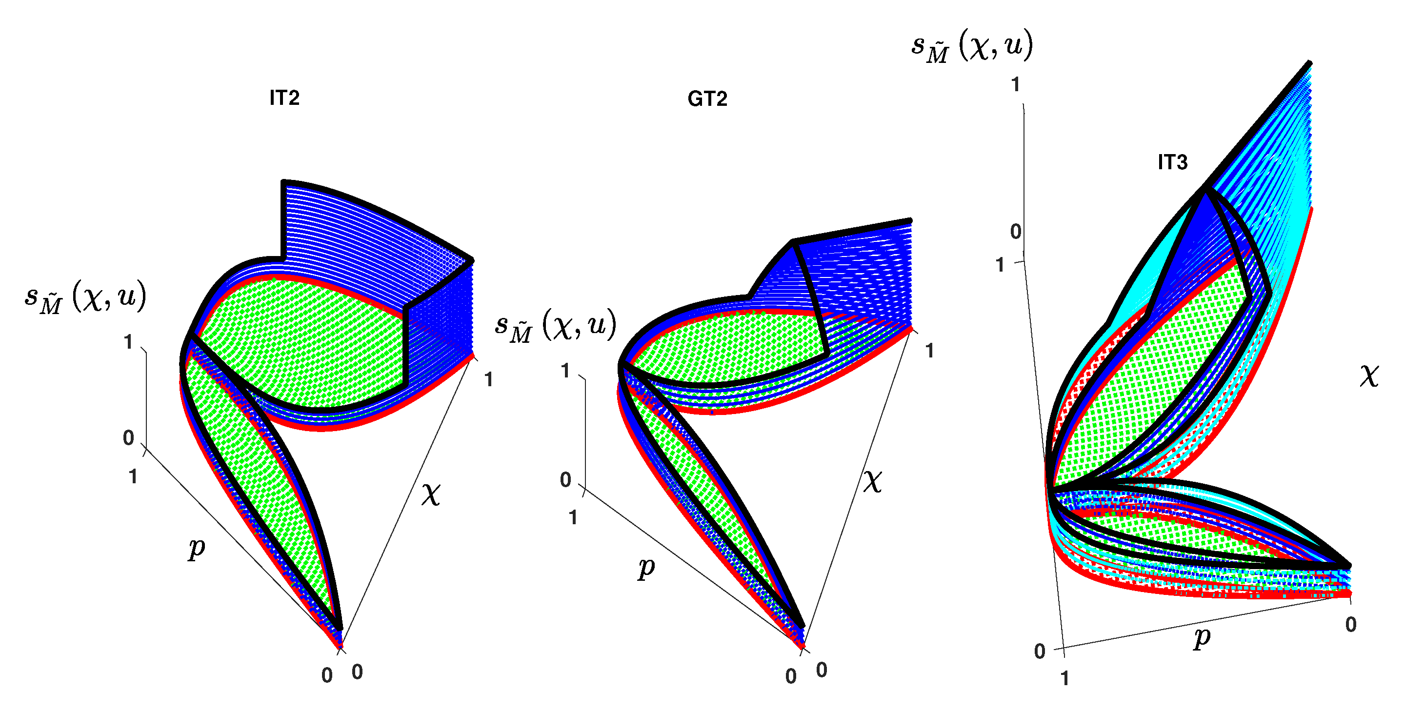
The other main difference is that the UB and LB of the footprint-of-uncertainty (FOU) in IT3-FSs are fuzzy numbers, but in IT2-FSs and GT2-FSs, they are crisp values. The FOU for three types of FS is depicted in Figure 2. Determining the upper/lower bounds of uncertainties is challenging in many problems. Then, the IT3-FSs can help us in situations where specifying the uncertainty range is a critical problem.
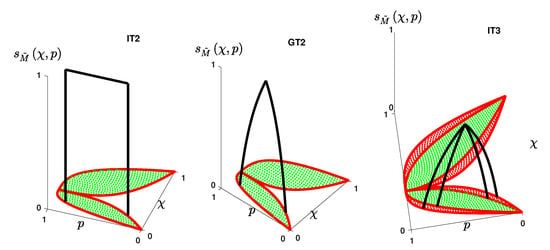
Figure 2.
FOU for IT2, GT2, and IT3 fuzzy sets.
Consider the membership function (MF) ; the various types of in the sense of IT2, GT2, and IT3 are written as given in Table 1.

Table 1.
Mathematical comparison of various type of MFs.
In Table 1, denotes the union on and p. As is seen from Table 1, the difference between the IT2-FS and GT2-FS is that the secondary MF is constant The difference between the interval and general type-2 MFs is the constancy of the secondary membership in the interval counterpart. In other words, in the IT2-FS, we have . In comparison with the type-3 FS, the secondary membership is a interval type-2 FS, and it is written as .
3. Proposed Type-3 FLS
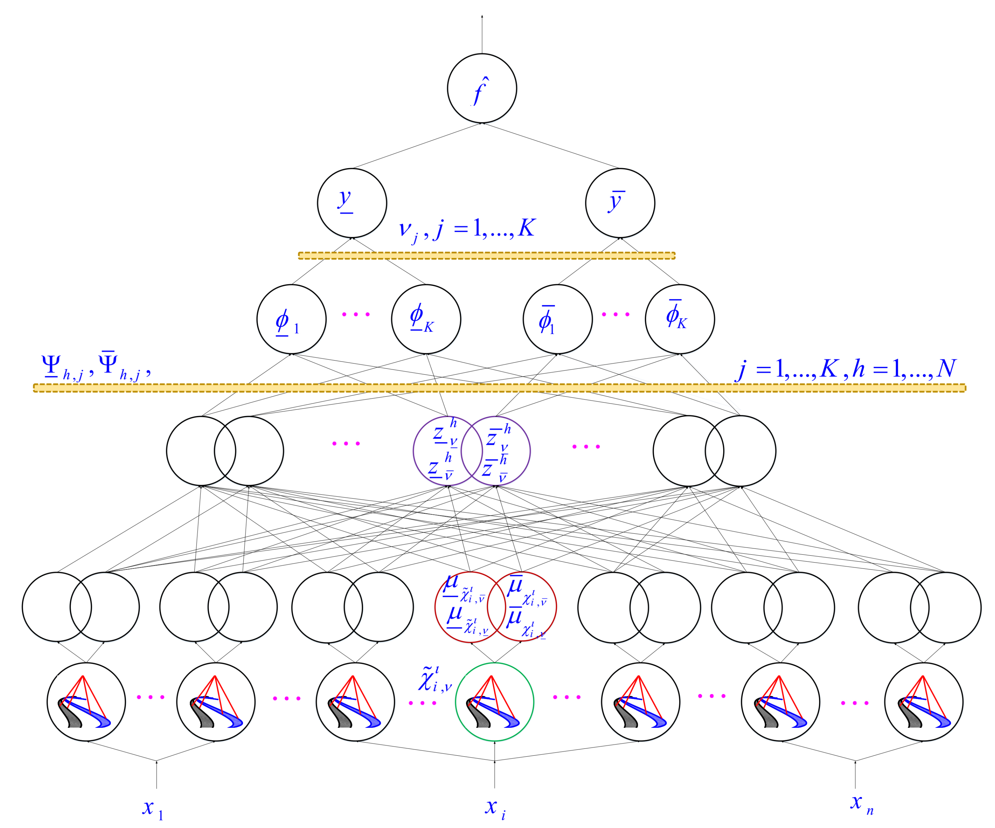
The general scheme is given in Figure 3. The UB and LB for the FOU in the type-3 membership functions (MFs) are not specific values, but they are interval fuzzy sets. Furthermore, the SM is a type-2 MF. The computation is summarized below:
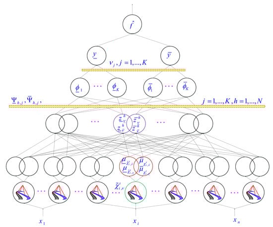
Figure 3.
Suggested T3-FLS.
(1) In the first step, obtain the inputs. The inputs are denoted by , .
(2) As shown in Figure 3, each input has MFs. The j-th MF input is denoted by . Following this, the memberships (firing degrees) are computed for . We have four primary memberships at each horizontal slice (secondary membership). Two values and denote the upper/lower bounds of the right side, and the two others and represent the upper/lower bounds of the left side. Following this, the memberships are computed for the suggested MF. The memberships for the MF, which are depicted in Figure 4, are computed as:
where is the center of and and are the widths of the left and right side of (see Figure 4). represent the value of the horizontal slice. and represent the width of the MFs. Small values of and result in narrow shapes of the MFs.
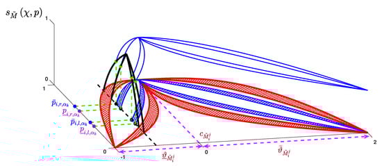
Figure 4.
Type-3 MF.
(3) Considering the memberships of the UB and LB of MFs , the rule firings are obtained as:
where , denote the -th MF for input . The h-th rule is given as:
where , , , and are the rule parameters. At each rule, the output is an interval type-3 fuzzy number, in which, its LB and UB are also fuzzy numbers. In other words, the LB belongs to , and the UB belongs to .
(4) The simplest estimation of the output is suggested as:
where
4. Learning Approach
In many problems, the rule parameters can be tuned by using derivative-based optimization methods. In these effective algorithms, the derivative of the output of the FLS needs to be calculated with respect to the rule variables. In this section, these computations are presented. The derivatives are obtained as:
5. How to Use T3-FLSs in Matlab Simulink
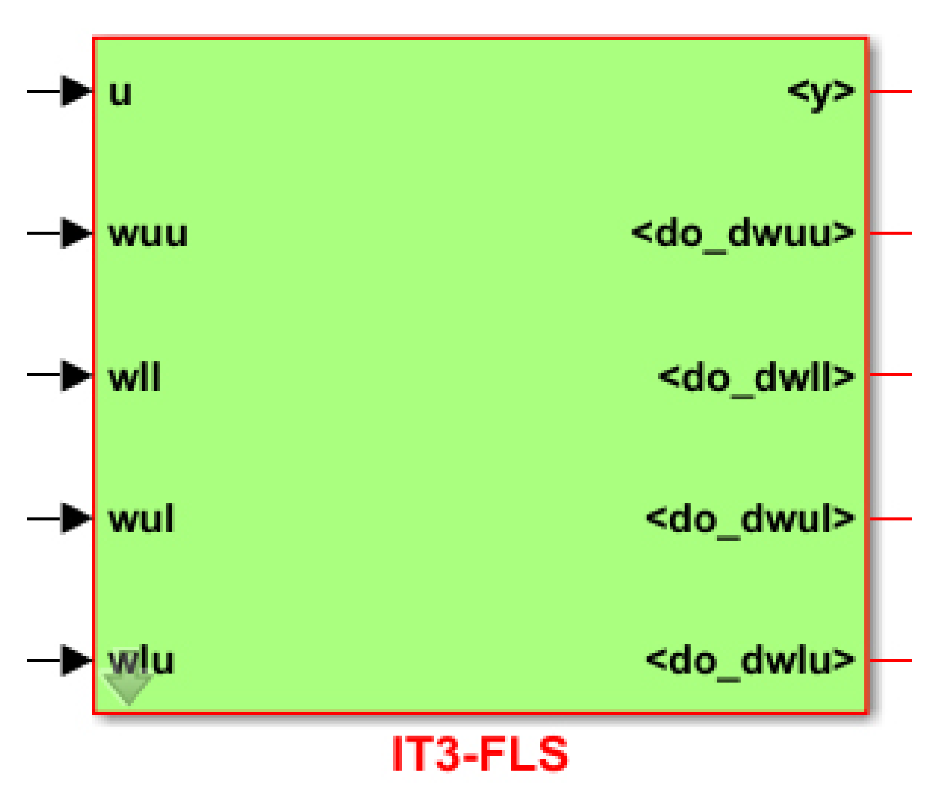
A practical Matlab implementation scheme is suggested in this section. The suggested toolbox can be easily used for various applications. The suggested scheme is shown in Figure 5. The output signals include the output of the T3-FLS and the derivatives of the output of the T3-FLS with respect to the rule variables, which can be used in the tuning laws.
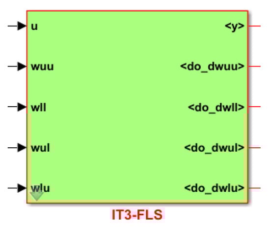
Figure 5.
Simulink block.
To illustrate how to use the designed toolbox easily, a simple example is presented as follows. Imagine a system with two inputs and . For input , two MFs are considered as and . For input , three MFs are considered as , , and . The horizontal slices are considered as , , and . For all MFs, the widths and are considered to be and , respectively (see (1)–(4)).
Now, assume the rules as follows:
- If is and is , then y is
- If is and is , then y is
- If is and is , then y is
- If is and is , then y is
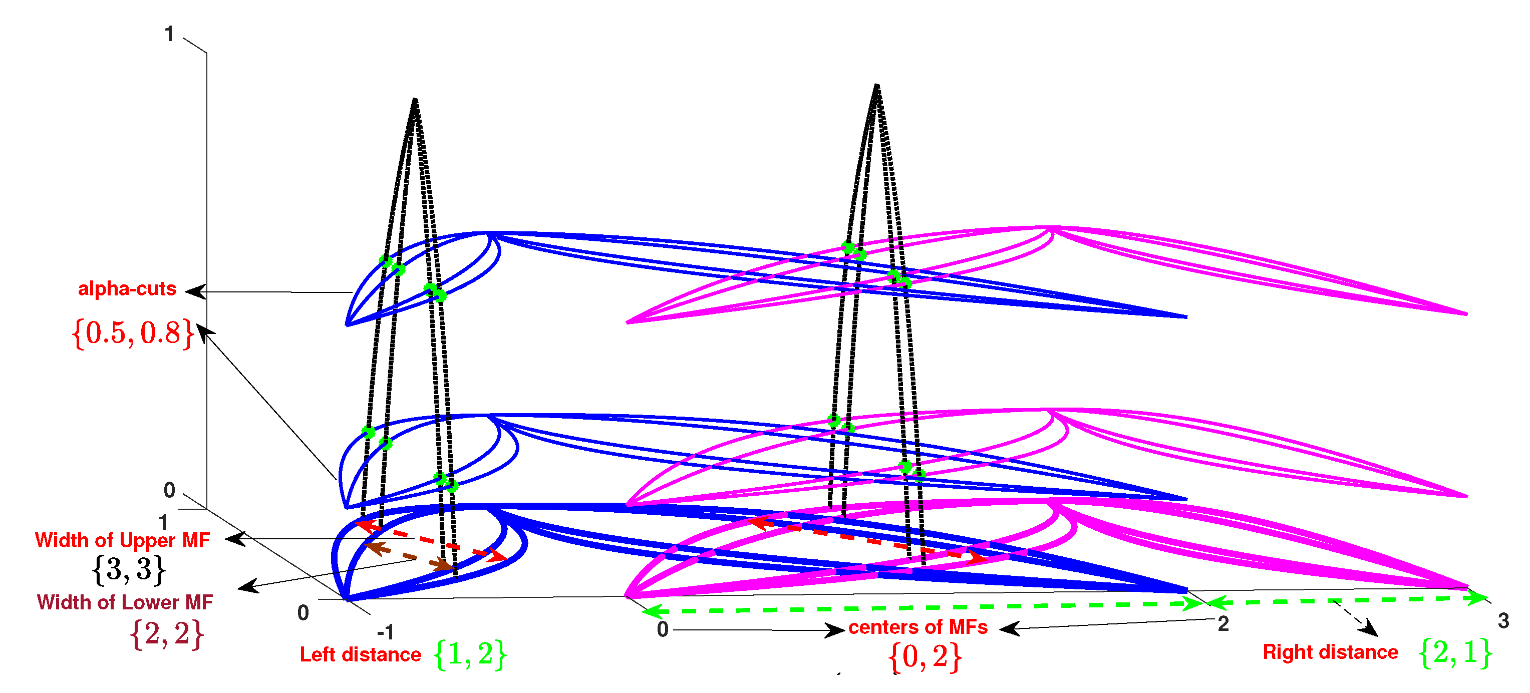
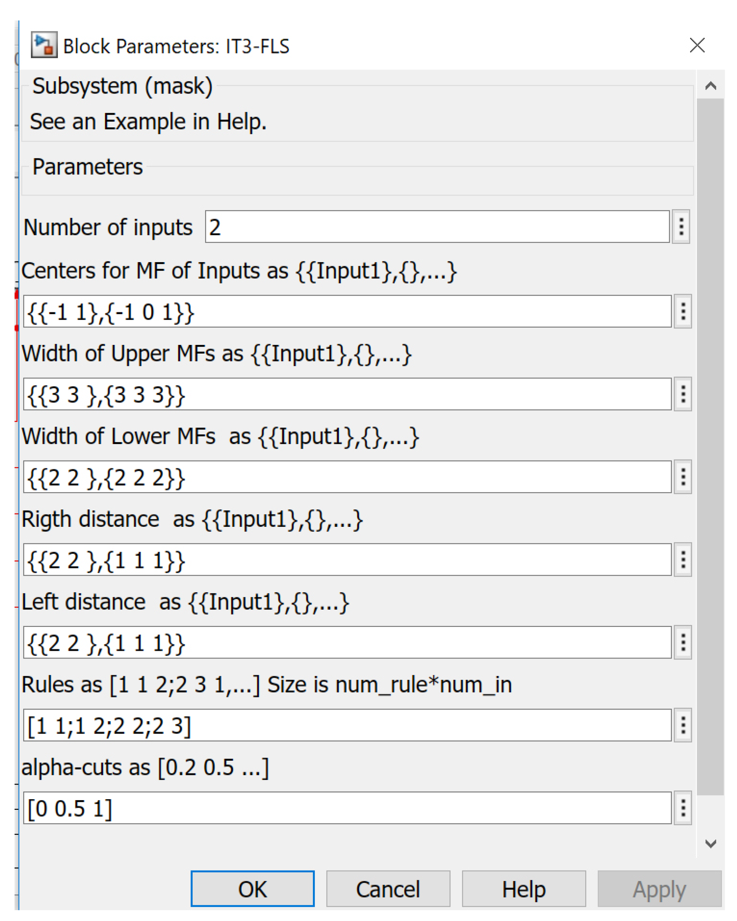
where is the j-th MF for i-th input. Therefore, in the designed toolbox, the information should be filled as follows (see Figure 6 and Figure 7):
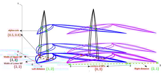
Figure 6.
An example for designing MFs.
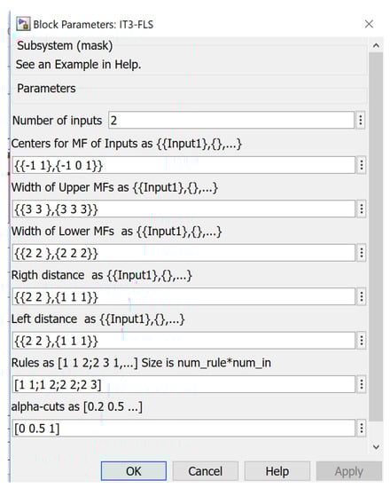
Figure 7.
Information of the IT3-FLS.
- Number of inputs: 2.
- Centers for MFs: {{−1 1},{−1 0 1}}, which means , , , , and .
- Rules: [1 1;1 2;2 2;2 3], which means, in the first rule, and are fired, in the second rule, and are fired, in the third rule, and are fired, and finally, in the last rule, and are fired.
- Alpha-cuts: [0 0.5 1], which means we have three horizontal slices and , , and .
6. How to Use T3-FLSs in Matlab M-File
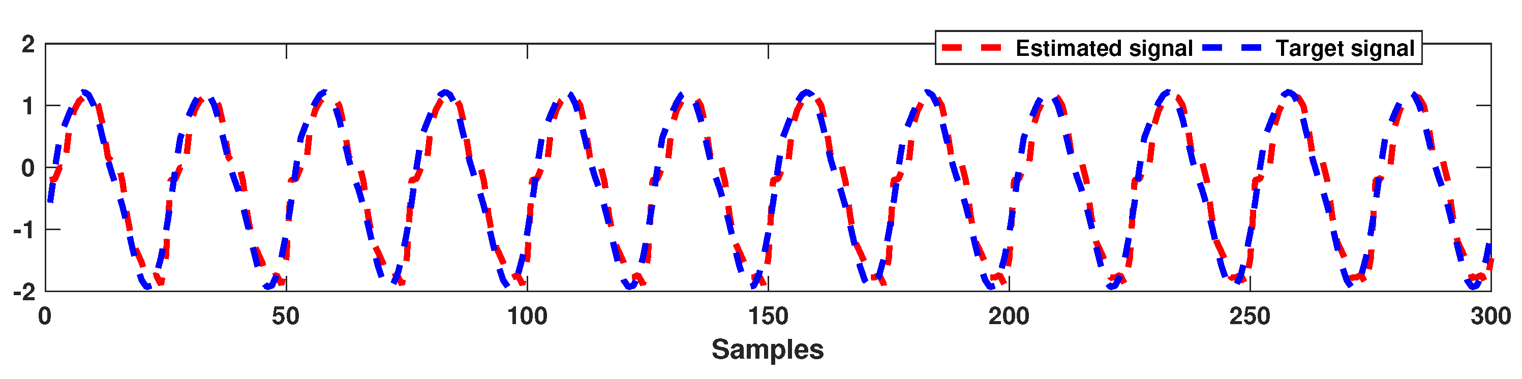
To practically use the T3-FLSs in various problems, a simple M-file code is presented. A modeling example is presented to illustrate better how to use the designed code. The problem is considered as the modeling of in (17). The input variables were considered as , and . The signal is defined as . The training/testing datasets are produced by and , respectively.
A Matlab function is presented as “out=Type3_FLS(u)”. For input “u”, the following information should be provided:
- u.x denotes the vector of inputs. In this problem, the number of inputs is three, then at each epoch, u.x is a vector with three elements.
- u.rules represent the rules, which are defined similarly to the previous section. For this problem, three rules are defined. The i-th rule is defined as:If is , is , and is , then is ;
Then, u.rules is defined as u.rules=[1 1 1;2 2 2; 3 3 3]:
- u.wuu, u.wll, u.wlu, and u.wul represent the vector of consequent parameters. u.wuu includes ; u.wll includes ; u.wul includes ; u.wlu includes .
In function “out=Type3_FLS(u)”, the signal “out” includes the estimated signal and the derivative of the output () with respect to the parameters of the rules (u.wuu, u.wll, u.wlu, and u.wul).
By executing the main program, the rule parameters are optimized, and the estimated and real signals are given as Figure 8.
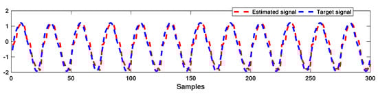
Figure 8.
The estimated and real signals.
7. Simulation
In this section, two examples are provided, to better show the effectiveness of the designed scheme for type-3 FLSs.
Example 1.
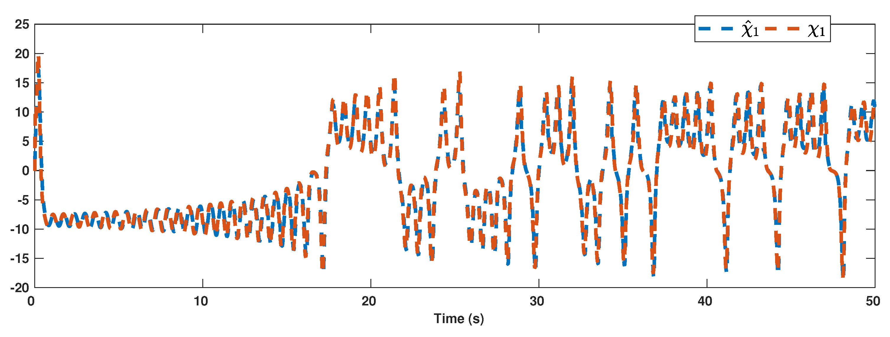
A simple simulation example is presented to show how to use the designed type-3 FLS. The suggested IT3-FLS is used to identify a chaotic system. The dynamics of the case study chaotic system is written as:
The inputs of the FLS were considered as , , and . For each input, three MFs are considered. The centers of the MFs for the first and second inputs are in −1, 0, and 1 and for the third input are in 0, 0.5, and 1. The left and right width of the MFs’ first and second inputs are 2 and for the third MF is 0.5. The number of alpha-cuts is three, and the values of alpha-cuts are considered as 0, 0.5, and 1. The number of rules is three, then we have 12 consequent parameters.
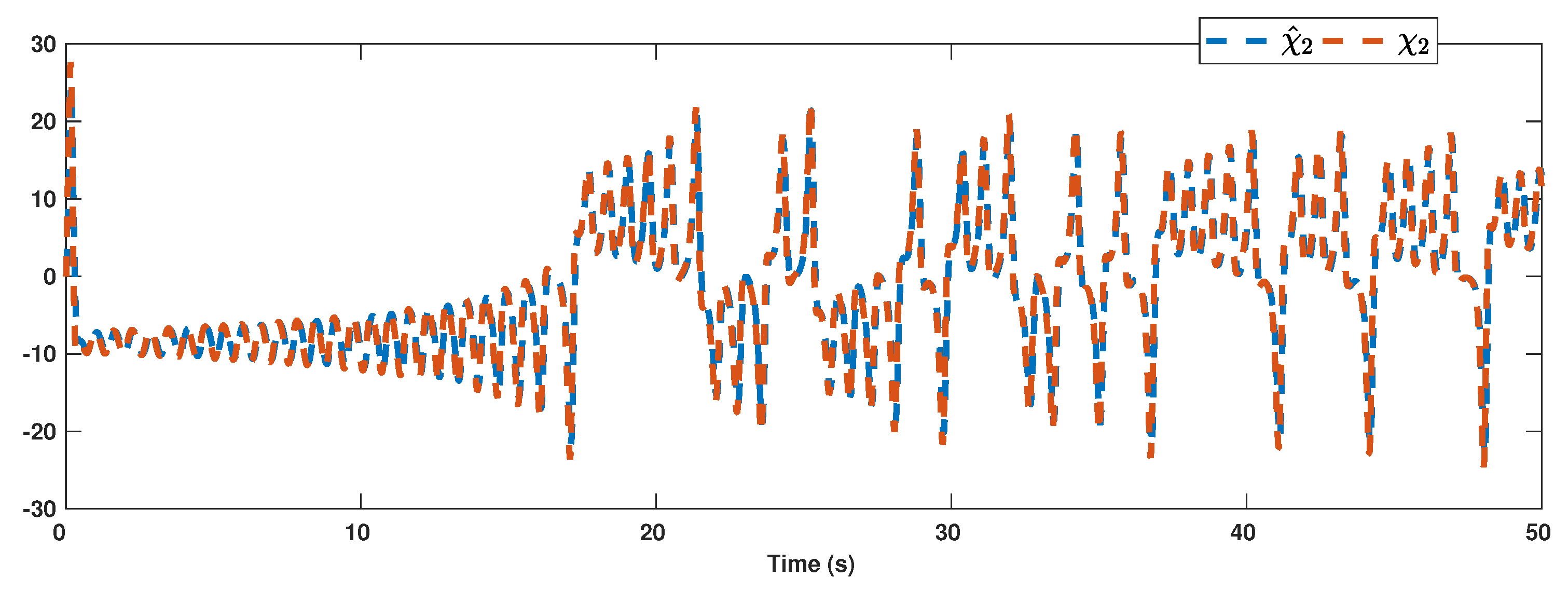
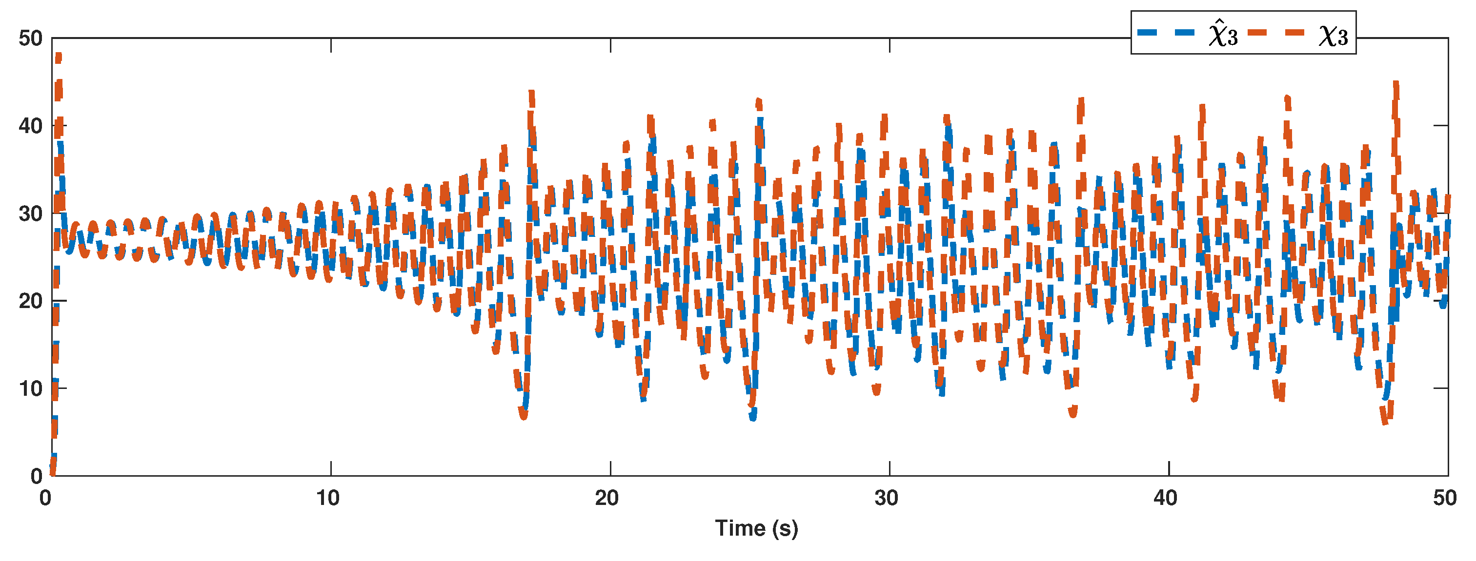
The simulation diagram is depicted in Figure 9. The signals are approximated by the IT3-FLS. The estimated trajectory and real signal are shown in Figure 10. The estimated trajectory and real signal are shown in Figure 11. The estimated trajectory and real signal are shown in Figure 12. It is seen that the suggested Simulink block works well in online applications.
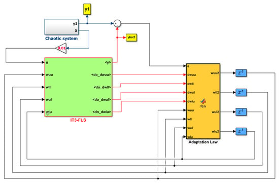
Figure 9.
Example 1: simulation diagram.

Figure 10.
Example 1: the estimation performance of .
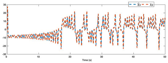
Figure 11.
Example 1: the estimation performance of .

Figure 12.
Example 1: the estimation performance of .
Example 2.

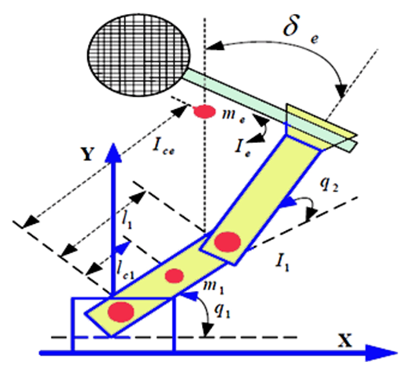
In this example, the suggested T3-FLS is used in a control application [23]. The suggested T3-FLS is used for the online control of a robotic manipulator [24]. The dynamics are written as (see Figure 13):
Figure 13.
Example 2: the case study robotic arm.
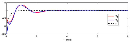
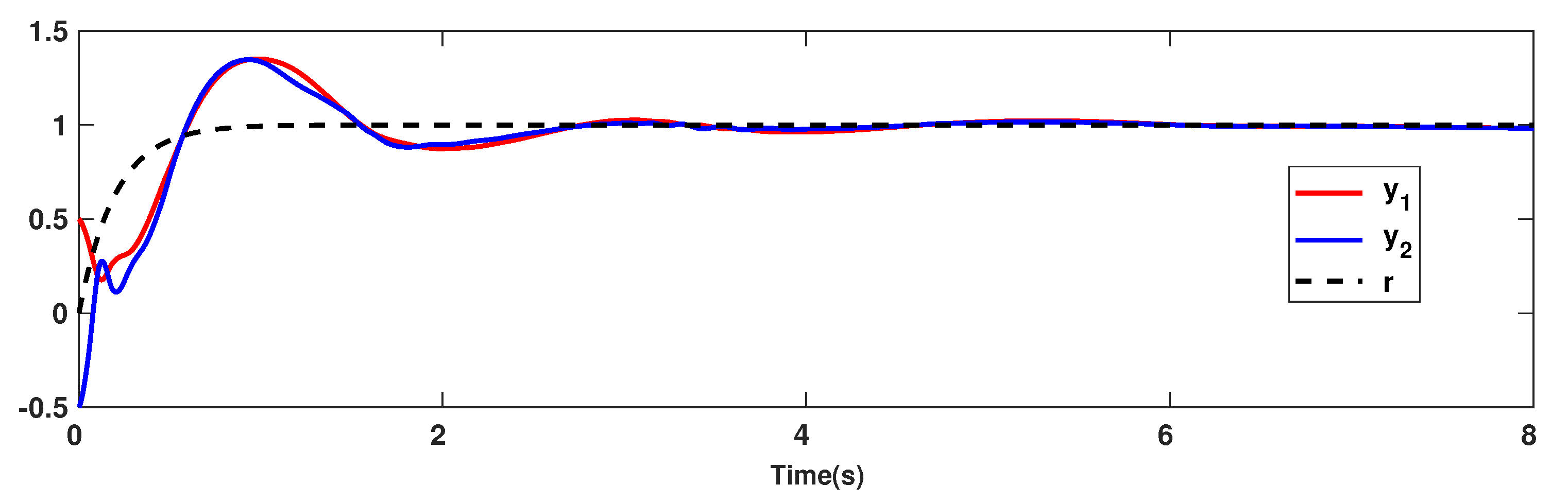
Figure 14.
Example 2: tracking performance.

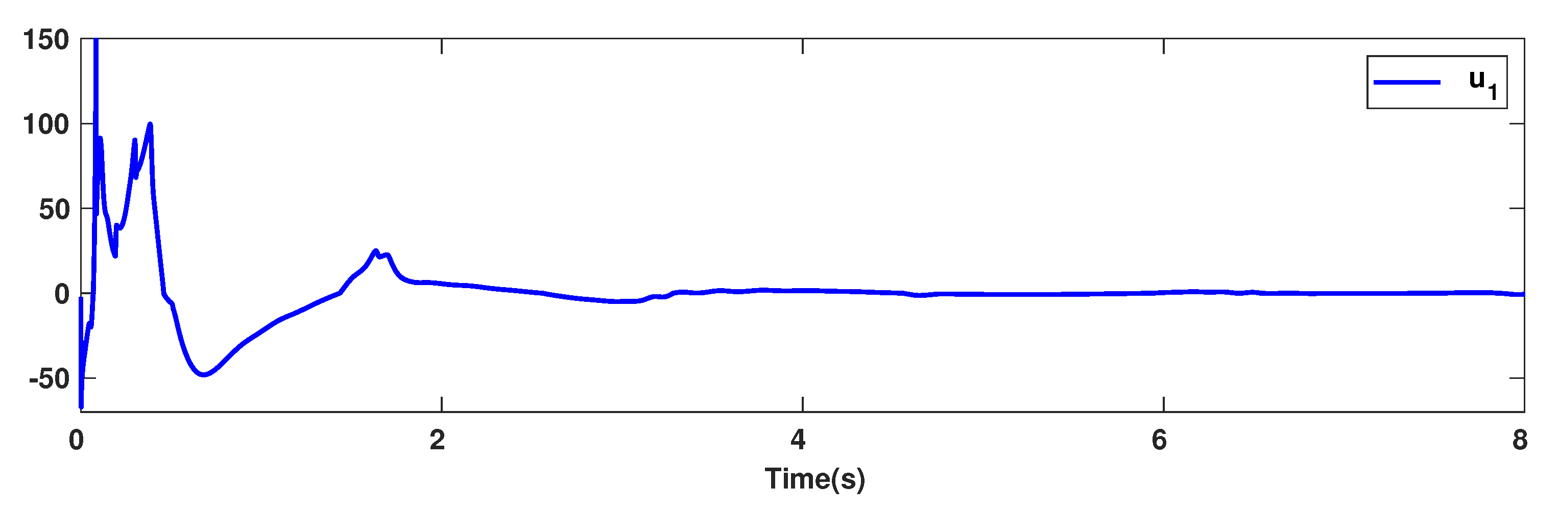
Figure 15.
Example 2: control signal .
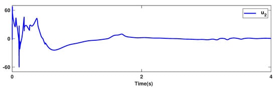
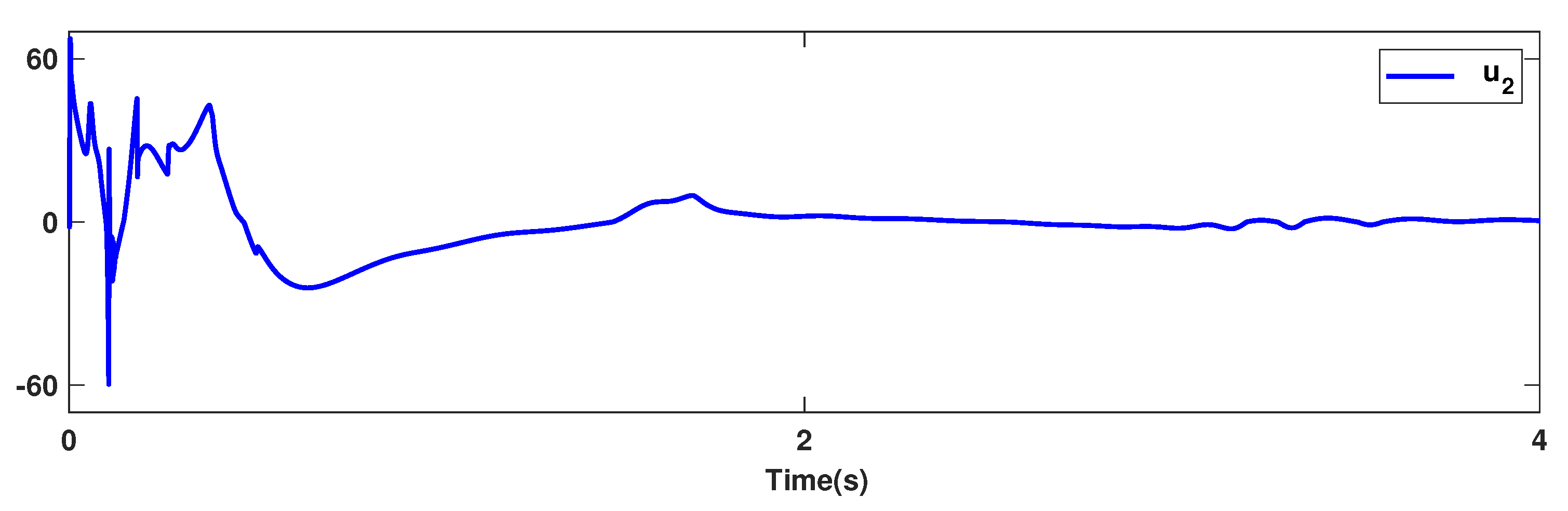
Figure 16.
Example 2: control signal .
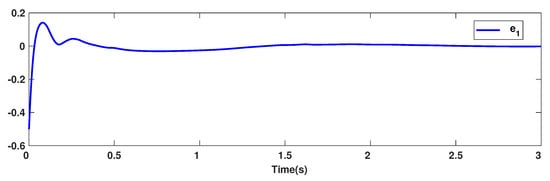
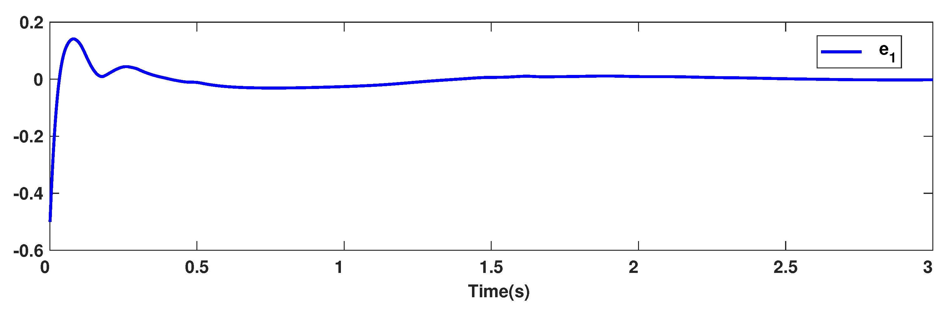
Figure 17.
Example 2: tracking error .
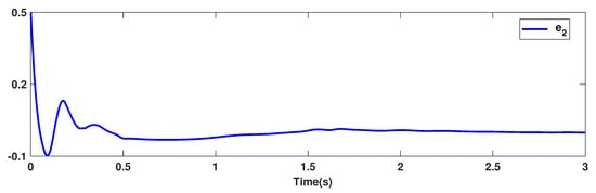
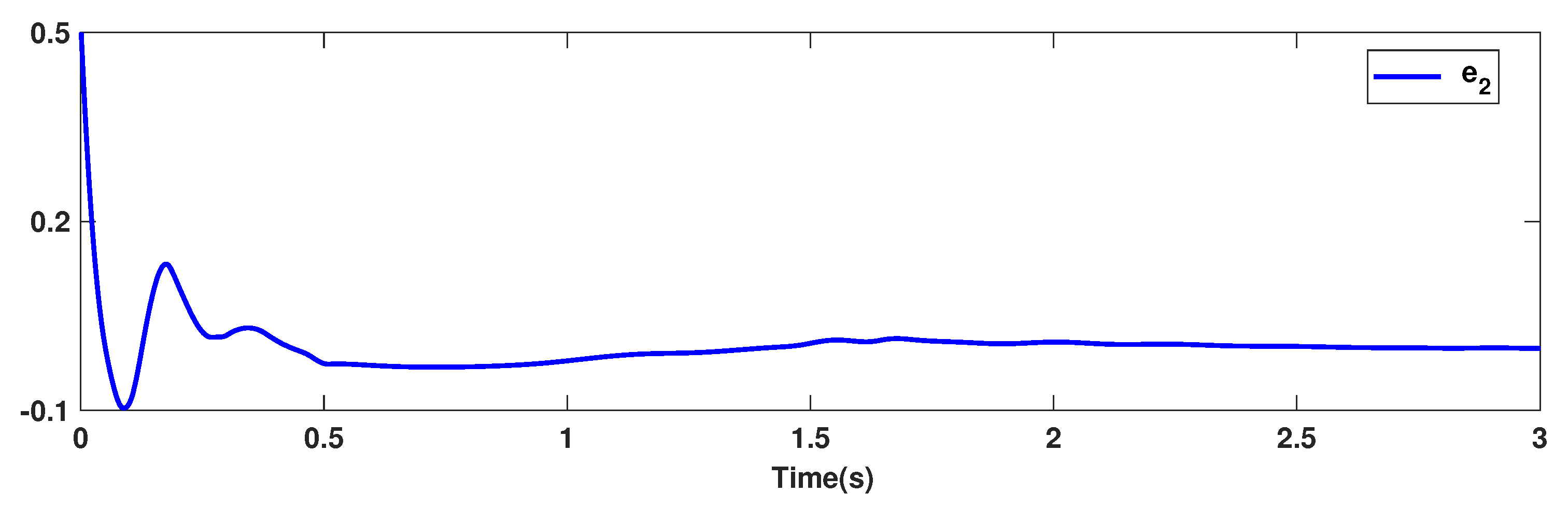
Figure 18.
Example 2: tracking error .
For future studies, the designed toolbox can be evaluated in machine learning applications [25], vibration control systems [26], optimization problems [26,27], mobile robots [28], and other engineering problems.
8. Conclusions
T3-FLSs have a significant potential for use in various uncertain modeling applications. However, there is no systematic approach to the design and use of T3-FLSs in practical applications. Therefore, in this paper, the simple and effective Matlab Simulink and M-files, by the illustrative and detailed examples, were given to implement the T3-FLSs. Furthermore, a comprehensive comparison was presented for various types of FLSs. Several graphical and mathematical examples were given to clarify the main differences. The computations of the memberships were simplified, and the derivative computations were presented to simplify the design of the adaptation laws. Two simulations demonstrated the usefulness of the T3-FLSs. In the first example, the suggested T3-FLSs were used for the identification of a chaotic system. The dynamics of the chaotic systems were considered fully uncertain like a black-box system. In the second example, the T3-FLS was used to design a simple controller. By the use of type-3 MFs, the linguistic variables were well converted to the mathematical equations, and by just two fuzzy rules, an effective fuzzy controller was designed. The simulation results demonstrated the effectiveness of T3-FLSs. It was shown that the T3-FLSs are a better choice in highly uncertain problems. Furthermore, the efficacy of the designed T3-FLSs in a control application was examined, and the good accuracy of the T3-FLSs was shown.
Author Contributions
Conceptualization, H.H., H.X., F.C., C.Z. and A.M.; methodology, H.H., H.X., F.C., C.Z. and A.M.; formal analysis, H.H., H.X., F.C., C.Z. and A.M.; writing—original draft preparation, H.H., H.X., F.C., C.Z. and A.M. All authors have read and agreed to the published version of the manuscript.
Funding
This research is financially supported by the Ministry of Science and Technology of China (Grant No. 2019YFE0112400), the Department of Science and Technology of Shandong Province (Grant No. 2021CXGC011204).
Data Availability Statement
Not applicable. No new data were created or analyzed in this study.
Conflicts of Interest
The authors declare no conflict of interest.
References
- Amador-Angulo, L.; Castillo, O.; Melin, P.; Castro, J.R. Interval Type-3 Fuzzy Adaptation of the Bee Colony Optimization Algorithm for Optimal Fuzzy Control of an Autonomous Mobile Robot. Micromachines 2022, 13, 1490. [Google Scholar] [CrossRef]
- Castillo, O.; Castro, J.R.; Melin, P. Interval Type-3 Fuzzy Systems: Theory and Design; Springer: Cham, Switzerland, 2022. [Google Scholar]
- Li, D.; Yu, H.; Tee, K.P.; Wu, Y.; Ge, S.S.; Lee, T.H. On time-synchronized stability and control. IEEE Trans. Syst. Man Cybern. Syst. 2021, 52, 2450–2463. [Google Scholar] [CrossRef]
- Zagui, N.L.S.; Krindges, A.; Lotufo, A.D.P.; Minussi, C.R. Spatio-Temporal Modeling and Simulation of Asian Soybean Rust Based on Fuzzy System. Sensors 2022, 22, 668. [Google Scholar] [CrossRef]
- Castillo, O.; Castro, J.R.; Melin, P. Forecasting the COVID-19 with Interval Type-3 Fuzzy Logic and the Fractal Dimension. Int. J. Fuzzy Syst. 2022, 25, 182–197. [Google Scholar] [CrossRef]
- Wu, Q.; Liu, X.; Qin, J.; Zhou, L. Multi-criteria group decision-making for portfolio allocation with consensus reaching process under interval type-2 fuzzy environment. Inf. Sci. 2021, 570, 668–688. [Google Scholar] [CrossRef]
- Leon-Garza, H.; Hagras, H.; Peña-Rios, A.; Conway, A.; Owusu, G. A type-2 fuzzy system-based approach for image data fusion to create building information models. Inf. Fusion 2022, 88, 115–125. [Google Scholar] [CrossRef]
- Bernal, E.; Lagunes, M.L.; Castillo, O.; Soria, J.; Valdez, F. Optimization of type-2 fuzzy logic controller design using the GSO and FA algorithms. Int. J. Fuzzy Syst. 2021, 23, 42–57. [Google Scholar] [CrossRef]
- Zhao, R.; Dai, H.; Yao, H. Liquid-metal magnetic soft robot with reprogrammable magnetization and stiffness. IEEE Robot. Autom. Lett. 2022, 7, 4535–4541. [Google Scholar] [CrossRef]
- Carvajal, O.; Melin, P.; Miramontes, I.; Prado-Arechiga, G. Optimal design of a general type-2 fuzzy classifier for the pulse level and its hardware implementation. Eng. Appl. Artif. Intell. 2021, 97, 104069. [Google Scholar] [CrossRef]
- Precup, R.E.; David, R.C.; Roman, R.C.; Szedlak-Stinean, A.I.; Petriu, E.M. Optimal tuning of interval type-2 fuzzy controllers for nonlinear servo systems using Slime Mould Algorithm. Int. J. Syst. Sci. 2021, 1–16. [Google Scholar] [CrossRef]
- Wan, S.P.; Chen, Z.H.; Dong, J.Y. An integrated interval type-2 fuzzy technique for democratic-autocrati multi-criteria decision making. Knowl.-Based Syst. 2021, 214, 106735. [Google Scholar] [CrossRef]
- Sennan, S.; Ramasubbareddy, S.; Balasubramaniyam, S.; Nayyar, A.; Abouhawwash, M.; Hikal, N.A. T2FL-PSO: Type-2 fuzzy logic-based particle swarm optimization algorithm used to maximize the lifetime of Internet of Things. IEEE Access 2021, 9, 63966–63979. [Google Scholar] [CrossRef]
- Pan, X.; Wang, Y. Evaluation of renewable energy sources in China using an interval type-2 fuzzy large-scale group risk evaluation method. Appl. Soft Comput. 2021, 108, 107458. [Google Scholar] [CrossRef]
- Mohammadzadeh, A.; Sabzalian, M.H.; Zhang, W. An interval type-3 fuzzy system and a new online fractional-order learning algorithm: Theory and practice. IEEE Trans. Fuzzy Syst. 2019, 28, 1940–1950. [Google Scholar] [CrossRef]
- Nabipour, N.; Qasem, S.N.; Jermsittiparsert, K. Type-3 fuzzy voltage management in PV/hydrogen fuel cell/battery hybrid systems. Int. J. Hydrogen Energy 2020, 45, 32478–32492. [Google Scholar] [CrossRef]
- Xu, W.; Qu, S.; Zhang, C. Fast terminal sliding mode current control with adaptive extended state disturbance observer for PMSM system. IEEE J. Emerg. Sel. Top. Power Electron. 2022, 11, 418–431. [Google Scholar] [CrossRef]
- Gheisarnejad, M.; Mohammadzadeh, A.; Farsizadeh, H.; Khooban, M.H. Stabilization of 5G telecom converter-based deep type-3 fuzzy machine learning control for telecom applications. IEEE Trans. Circuits Syst. II Express Briefs 2021, 69, 544–548. [Google Scholar] [CrossRef]
- Gheisarnejad, M.; Mohammadzadeh, A.; Khooban, M. Model Predictive Control-Based Type-3 Fuzzy Estimator for Voltage Stabilization of DC Power Converters. IEEE Trans. Ind. Electron. 2021, 69, 13849–13858. [Google Scholar] [CrossRef]
- Castillo, O.; Castro, J.R.; Melin, P. A methodology for building interval type-3 fuzzy systems based on the principle of justifiable granularity. Int. J. Intell. Syst. 2022, 37, 7909–7943. [Google Scholar] [CrossRef]
- Tian, M.W.; Mohammadzadeh, A.; Tavoosi, J.; Mobayen, S.; Asad, J.H.; Castillo, O.; Várkonyi-Kóczy, A.R. A deep-learned type-3 fuzzy system and its application in modeling problems. Acta Polytech. Hung. 2022, 19, 151–172. [Google Scholar] [CrossRef]
- Peraza, C.; Ochoa, P.; Castillo, O.; Geem, Z.W. Interval-Type 3 Fuzzy Differential Evolution for Designing an Interval-Type 3 Fuzzy Controller of a Unicycle Mobile Robot. Mathematics 2022, 10, 3533. [Google Scholar] [CrossRef]
- Duan, J.; Duan, G.; Cheng, S.; Cao, S.; Wang, G. Fixed-time time-varying output formation-containment control of heterogeneous general multi-agent systems. ISA Trans. 2023, in press.
- Wang, J.; Yang, M.; Liang, F.; Feng, K.; Zhang, K.; Wang, Q. An algorithm for painting large objects based on a nine-axis UR5 robotic manipulator. Appl. Sci. 2022, 12, 7219. [Google Scholar] [CrossRef]
- Dang, W.; Guo, J.; Liu, M.; Liu, S.; Yang, B.; Yin, L.; Zheng, W. A semi-supervised extreme learning machine algorithm based on the new weighted kernel for machine smell. Appl. Sci. 2022, 12, 9213. [Google Scholar] [CrossRef]
- Meng, Q.; Lai, X.; Yan, Z.; Su, C.Y.; Wu, M. Motion planning and adaptive neural tracking control of an uncertain two-link rigid–flexible manipulator with vibration amplitude constraint. IEEE Trans. Neural Netw. Learn. Syst. 2021, 33, 3814–3828. [Google Scholar] [CrossRef] [PubMed]
- Lu, S.; Guo, J.; Liu, S.; Yang, B.; Liu, M.; Yin, L.; Zheng, W. An improved algorithm of drift compensation for olfactory sensors. Appl. Sci. 2022, 12, 9529. [Google Scholar] [CrossRef]
- Wang, J.; Liang, F.; Zhou, H.; Yang, M.; Wang, Q. Analysis of Position, pose and force decoupling characteristics of a 4-UPS/1-RPS parallel grinding robot. Symmetry 2022, 14, 825. [Google Scholar] [CrossRef]


Disclaimer/Publisher’s Note: The statements, opinions and data contained in all publications are solely those of the individual author(s) and contributor(s) and not of MDPI and/or the editor(s). MDPI and/or the editor(s) disclaim responsibility for any injury to people or property resulting from any ideas, methods, instructions or products referred to in the content. |
© 2023 by the authors. Licensee MDPI, Basel, Switzerland. This article is an open access article distributed under the terms and conditions of the Creative Commons Attribution (CC BY) license (https://creativecommons.org/licenses/by/4.0/).