Abstract
In this paper, the control of robotic manipulators (RMs) is studied. The RMs are widely used in industry. The RMs are multi-input-multi-output systems, and their dynamics are highly nonlinear. To improve the accuracy in practice, it is impossible to ignore the influence of nonlinear dynamics and the interaction of inputs–outputs. Non-structural uncertainties such as friction, disturbance, and unmodeled dynamics are other challenges of these systems. Recently, type-3 (T3) fuzzy logic systems (FLSs) have been suggested that result in better accuracy in a noisy environment. In this paper, a new control idea on the basis of T3-FLSs is suggested. T3-FLSs are used to estimate the dynamics of RMs and the symmetrical perturbations. The T3-FLSs are learned using online laws to enhance the stability. To eliminate the effect of the interconnection of inputs and estimation errors, a compensator is developed. By several simulations, the superiority of the suggested controller is demonstrated.
1. Introduction
Robot arms that are driven by electric motors without gears are called direct drive robots. These robots show better performance by eliminating flexibility, clearance, and the retraction of gears, reducing friction, reducing inertia, and increasing reliability. The robot arm is a complex system with nonlinear dynamics and uncertainty. This irregular and unpredictable behavior of the robot is ineffective in practice and shows the importance of control. It is expected that the robot will perform industrial tasks with high accuracy and speed. Fuzzy control is one of the robot-control methods that has attracted researchers’ attention as an intelligent method. This control method is independent of the dynamic model in design and shows good performance [1,2].
Robot arms can be classified in terms of geometry, kinematic structure, the type of application, and the control method [3]. In terms of geometry, we can refer to the configuration of the artist, cylindrical, spherical, Cartesian, and Scara. Direct kinematics and inverse kinematics are used to determine the final position and direction of the robot arm. In the first case, for having the variable values of the joints, the position and direction of the final operator are determined, but in the second case, for having the position and direction of the final operator, the values of the variables of the joints are obtained. To describe the dynamic of the RM by analyzing the potential energy and kinetic energy of the robot arm, its dynamic equation is obtained and its behavior is checked. There are two types of robot arms with direct and indirect thrust [4,5]. Direct drive ones are arms equipped with electric motors without a power transmission system, which show better performance by eliminating gear backlash, reducing friction, reducing inertia, and increasing reliability, causing the precise control of torque and increasing speed [6,7].
To use a robot arm for any purpose, it is necessary to control its movement. Depending on the conditions and application, motion control can be done with the two goals of adjusting and tracing the desired path [8,9]. For example, in a foundry, when the goal is to keep the container in which the molten material is poured, in a fixed place under the melting furnace, it is a control issue of the adjustment type. When the goal is to paint a car robot arm in an automobile factory, the robot must follow a predetermined path. Here, the tracking problem must be solved. Of course, the adjustment problem can be considered a special case of the tracking problem. Therefore, solving the problem of tracking in the control of robot arms is of special importance, and for this reason, in the control literature, this problem has been solved by different methods [10].
The analysis of the stability and control of nonlinear systems has always been a challenge for mathematical and engineering researchers, especially control engineers, due to the specific complexities of these systems and the existence of different behaviors in their different working points. Controller design to guarantee the robustness and optimal efficiency of a non-linear system generally require special and complex mathematical and engineering knowledge. The theory of stability with the direct and indirect methods of Lyapunov can perhaps be introduced as the only powerful theoretical tool available to analyze the stability of equilibrium points of a nonlinear system. In addition, many methods of designing non-linear control systems are somehow dependent on finding a Lyapunov function that satisfies certain conditions. Meanwhile, finding the appropriate Lyapunov function for stability analysis and controller design for nonlinear systems is not an easy task, and there is still no systematic method for this task. Therefore, paying attention to these theoretical complexities is not so easy for engineers working in the industry to understand these theoretical topics and more importantly apply them in industrial applications [11,12].
Non-adaptive and adaptive control are two subcategories of FLS-based controllers. The structure and settings of the FLS-based controller are fixed and will not change throughout the real-time operation in non-adaptive FLS-based control. When using adaptive fuzzy control, the fuzzy controller’s structure and parameters are modified in response to the circumstances encountered during real-time application. Compared to adaptive control, non-adaptive control is easier to use, but it requires more data from the process model and heuristics. On the other hand, adaptive FLS-based control is expensive to implement, but at the same time, it requires less information; as a result, it may be implemented better and more effectively. FLS-based controller design methods are classified into two categories: the trial–error method and the theory method. In the trial–error method, using experimental knowledge and the information of experts, detailed questionnaires are prepared and a set of rules if-then the fuzzy is collected. Then, fuzzy controllers are built based on these rules and finally tested in the system. Then, if the application of the designed FLS-based controller is not satisfactory in practice, the rules are changed and adjusted appropriately or created again from the beginning, and this process continues until after several cycles of trial–error, the final efficiency is desired. In the theoretical method, the parameters and structure of FLS-based controllers are schemed in such a way that a specific accuracy criterion is guaranteed. Of course, it is better to combine both methods in the design of fuzzy controllers for practical systems in order to achieve the best FLS-based controller [13,14].
2. Literature Review
The model-based fuzzy controllers are widely used in various problems [15,16]. For example, the goal of [17] is to investigate a terminal sliding mode control (SMC) technique for a RM with unknown disturbances. First, because FLS-based wavelet neural networks have better function approximation capabilities, the authors employ them to assess dynamic uncertainty. By altering the weights online, the authors secondly construct the adaptive controller to reduce external disturbances. The cooperative robotic manipulators with unclear base coordinates is examined in [18]. Given unknown coordinate uncertainties, an adaptive controller is suggested to predict the parameters. The internal forces are stabilized by a robust SMC based on synchronisation factors. Under various circumstances, mathematical experiments are carried out. The paper [19] suggests a discrete-time controller that depends on well-known mechanical system structural characteristics but ignores any prior knowledge of the system parameter values. Additionally, a FLS formulation is taken into account to account for outside disruptions. Online adjustments are made to the FLS outputs to enhance the response. Finally, example simulations are examined to show that the suggested technique is workable. To regulate the position tracking of robot manipulators in the presence of uncertainty, the paper [20] introduces a high-speed adaptive fuzzy SMC. The dynamics are split into two subsystems and then linked together with the use of an intermediary variable. The singularity is then removed, the tracking speed is increased, and a fuzzy approximator is suggested to lessen the chattering phenomena in the input signal. Finally, a fuzzy-logic controller (FLC) with just one adaptive rule is suggested to approximate the uncertainties. This FLC is capable of overcoming the uncertainty effect and eliminating the chatting phenomena.
To increase the accuracy under the motion constraint, the authors of [21] suggest a control system that combines a predictive controller with an FLS approximation. In order to manage the kinematic uncertainty included in the MPC control, the fuzzy approximation is implemented. To validate the suggested algorithm, simulations are then run and assessed. In contrast, the outcomes show that the suggested algorithm succeeds and performs satisfactorily in the presence of outside disturbances. In [22], a dynamic surface control-based adaptive backstepping FLC is presented to follow and operate the RM while taking into account uncertainties. First, the RM model is split into first-order subsystems using a feedback control approach, and the control inputs that need to be constructed are presented. Second, two FLSs are used to estimate the unknown modelling mistakes, and it is believed that the external disturbances are below a specific upper limit. Thirdly, this article employs a dynamic surface control approach to mitigate the age-old issue of “explosion of complexity” in the design of the backstepping scheme. The Lyapunov theory is then used to show that the suggested controller is stable.
In [23], an FLC is used to stabilize the armature current. The FLC input is the armature current and position error. The structure of this controller is resistant to RM uncertainties, and the simulation results verify the satisfactory performance of this controller. In [24], the combination of the computational torque control and the FLC is used, the global stability is provided by the computational torque component, and the FLC overcomes the uncertainties. The simulations demonstrate the good tracking ability of this controller. In [25], a Takagi–Sugno robust fuzzy controller for tracking and adjustment control is designed for the robot arms, and the analysis of FLC as a robust controller is shown by direct Lyapunov method. Additionally, the voltage control strategy is used instead of the torque controller, which eliminates the complexity in the analysis and the design of the controller. The simulation results show the proper performance of this controller. In [26], the decentralized direct adaptive FLC for electric robot arms using a voltage control strategy is proposed. The current space model of the robot system includes the robot arm and hair nets, in a non-combined, multi-variable, highly non-linear form, heavy coupling, and with a variable input gain matrix. Adaptive fuzzy control suffers from computational load due to the use of all current variables. A controller was presented to overcome these problems, which, in addition to simplicity, has an accurate response, robust performance, and guarantees stability. Additionally, instead of all current variables, only the error and its derivative, i.e., the controller input, are considered. The simulation results attribute the superiority of this method to proportional-derivative FLC. In [27], the fuzzy SMC is used to control the robot arm. One of the superiorities of this controller is guaranteeing stability and correcting tracking errors. The simulation results show the flexibility and robustness of this method compared to FLC and SMC.
The type-2 FLSs (T2-FLSs) have better capability in comparison with their type-1 counterparts. In few studies, T2-FLS are used for RM. For example, the trajectory tracking control issue of planar underactuated RMs is the subject of [28]. First, a somewhat linearized version of the dynamic model is created. The linearized system is then developed using a type-1 FLC using a linear quadratic regulator controller. Then, in order to deal with uncertainties, an interval T2-FLC is developed by blurring the fuzzy sets of type-1 FLC. Simulations are used to validate the suggested type-1 and interval T2-FLC and to compare them to one another, particularly when system uncertainties are present. An automated control approach is suggested in [29] for an RM based on T2-FLS and SMC. Unmodulated dynamics, and undetermined parameters, are approximated by a T2-FLS. The effectiveness of the suggested technique has been tested in simulations under a variety of conditions, including ambiguity in the arm parameters, ambiguity in the RM parameters, ambiguity in the load, and ambiguity in the modelling. The suggested method’s effectiveness and superiority are demonstrated by comparison with two traditional controllers. The study [30] aids in the design of an adaptive supervisory FLS-based SMC. It is suggested that the FLC create switching control signals without encountering the chattering issue. To achieve this, an adaptive method is recommended for the online adjusting of the SMC’s output gain. Additionally, a supervisory control system is taken into consideration for the online tweaking of the PID sliding surface gains in order to improve tracking. It is advised to use the Grasshopper Optimization Algorithm to improve the membership functions chosen for the fuzzy sliding surface. Using the Lyapunov stability theorem, the closed-loop system’s stability is demonstrated. The benefits of the suggested controller in terms of decreased chatter are demonstrated by simulation results. A finite-time adaptive T2-FLC is presented in [31] via a backstepping approach to address the tracking issue of a robot. The complex dynamics of the robot are approximated using an interval T2-FLS based approximator, and the output is derived using an enhanced Begian–Melek–Mendel reduction technique. The suggested controller is relatively simple to use and has a broad variety of applications because it only depends on the robot’s length, breadth, and wheel radius, which are readily available and time-invariant. The practical semi-global finite-time stability theory establishes the stability. The main advantages of the suggested scheme are as follows:
- A new T3-FLC is presented for RMs that does not depend on the dynamics of RMs.
- The influence of nonlinear dynamics and the interaction of inputs–outputs are handled.
- The T3-FLSs are learned using online laws to enhance their stability.
- To eliminate the effect of the interconnection of inputs and the estimation errors, a compensator is developed.
- The suggested T3-FLS-based controller has better efficiency in a noisy condition.
3. Problem Formulation
In this paper, we study 2 degrees of freedom RM, which are more popular in industry. However, the designed scheme can be extended for other RMs. The dynamic equations are written as follows:
The dynamics are rewritten as:
where and denote the disturbances and
The Equation (12) are rewritten as:
where and are the reference signals; , , and are the estimations of , , and , respectively; and
If the functions , , , and are known, then the ideal controllers can be:
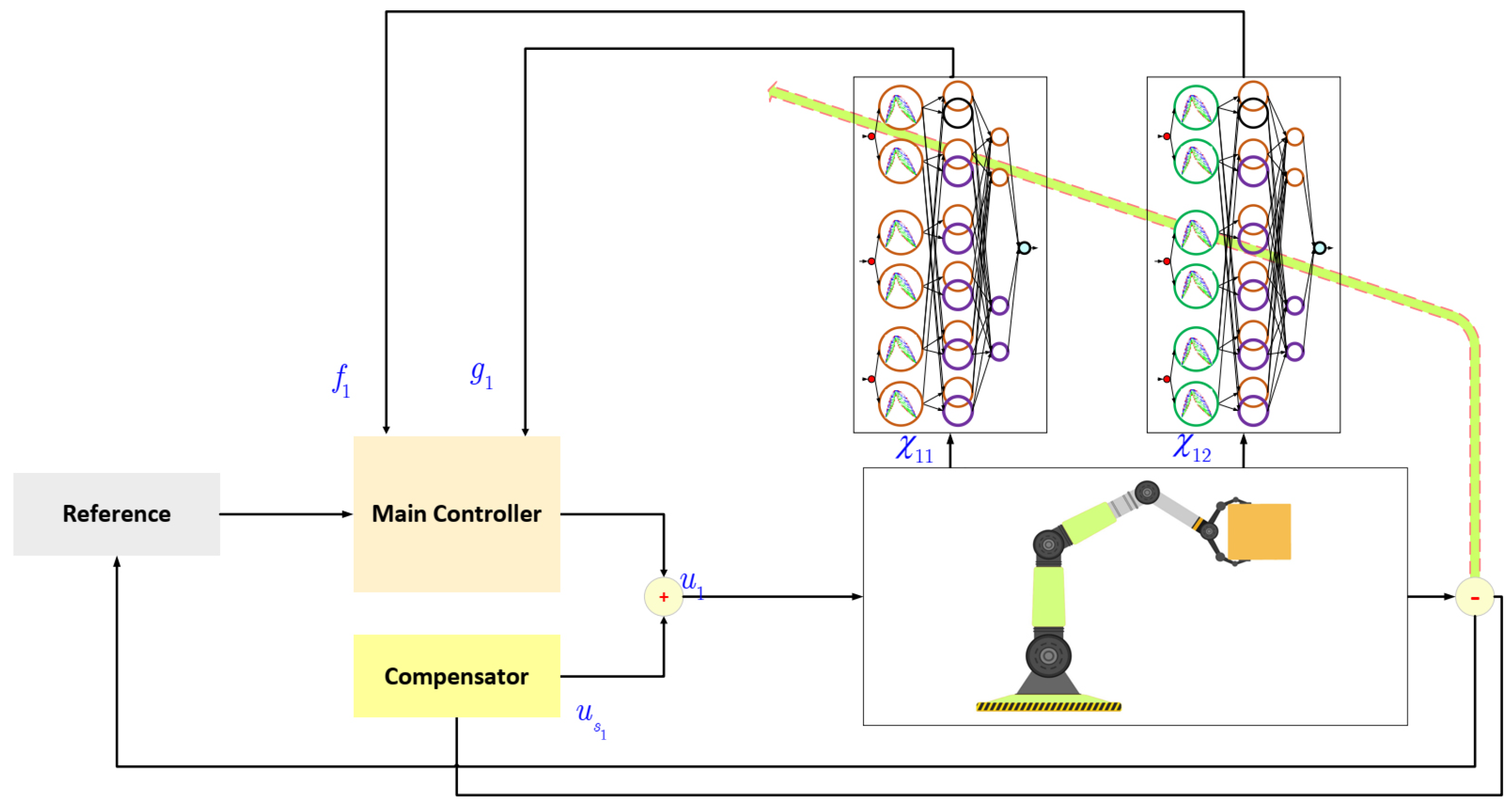
where , selected such that is Hurwitz-stable. The suggested scheme is shown in Figure 1. Since the functions , , , and are unknown, the dynamics are perturbed by and , and the control signals are modified as follows:
where , , , and are the estimation of , , , and , respectively. is a small constant, and is defined as:
and are compensators.
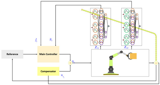
Figure 1.
Suggested control scheme.
4. Type-3 FLS
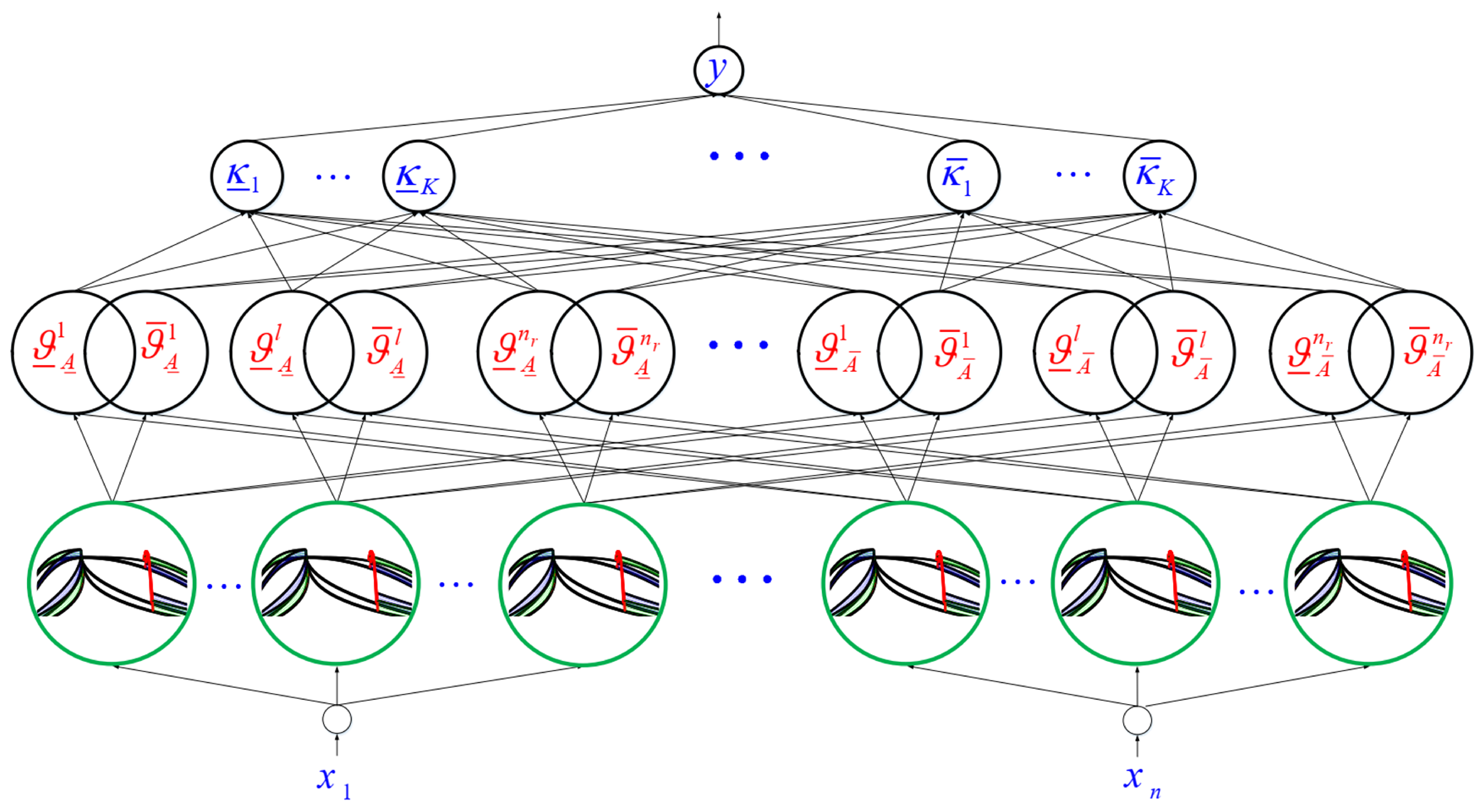
The theory of fuzzy sets is a theory for action under uncertainty. This theory mathematically formulates many imprecise concepts and variables and systems. The three types of fuzzy systems used in FLC are pure fuzzy systems, Takagi–Sugno FLSs, and Mamdani FLSs. In the Takagi–Sugno FLSs, the “then” part is the rule of the mathematical representation and then does not give a scheme for humanistic representation. Additionally, it does not leave the designer’s hand free to apply different logics, and as a result, the flexibility of FLS is not present in this structure. Mamdani’s FLS solves the problem of the previous two systems by placing a fuzzifier and a non-fuzzifier in the input/output of the FLS inference meter. The T3-FLSs are used to estimate the uncertainties. The following main equations are presented (see Figure 2).
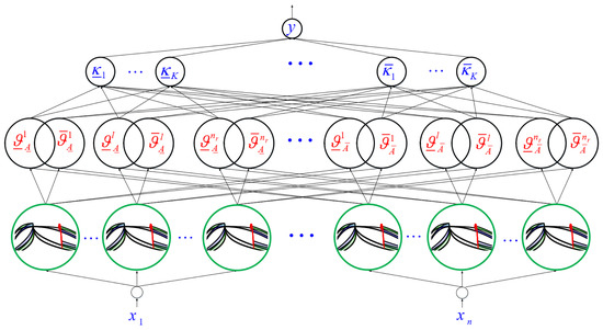
Figure 2.
Type-3 FLS.
Step 1: The inputs of T3-FLSs are as .
Step 2: The memberships for , are computed as (see Figure 3):
where and / denote the and distances of to the left/right points, respectively.
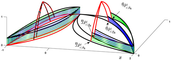
Figure 3.
Type-3 MF.
Step 3: The upper/lower rule firings are obtained as:
where , denotes the level of slices.
Step 4: The output is:
where
where K/ denotes the number of slices/rules.
5. Stability
By adding and subtracting and , we have:
The optimal error is defined as:
For stability analysis, we consider:
where , , , , denote the upper bound of , , , , , respectively. The other variables are defined as: , , , . The matrices , , , are obtained as:
where
Derivative of (49), yields:
The tuning rules are considered as:
Then, we have:
in (56) can be written as:
The adaptation laws are considered as:
By substituting the adaptation laws (61), we have:
Regarding the boundedness of errors, from the Barbalat’s lemma [32] the stability is proved.
Remark 1.
In this paper, we considered 2-degree of freedom RMs. However, the designed controller can be extended for other more degree of freedom RMs. The main point is that dynamics of each output can be modeled by the suggested T3-FLSs.
6. Simulation
The simulation parameters are considered as:
The reference is considered as , and the control patenters are:
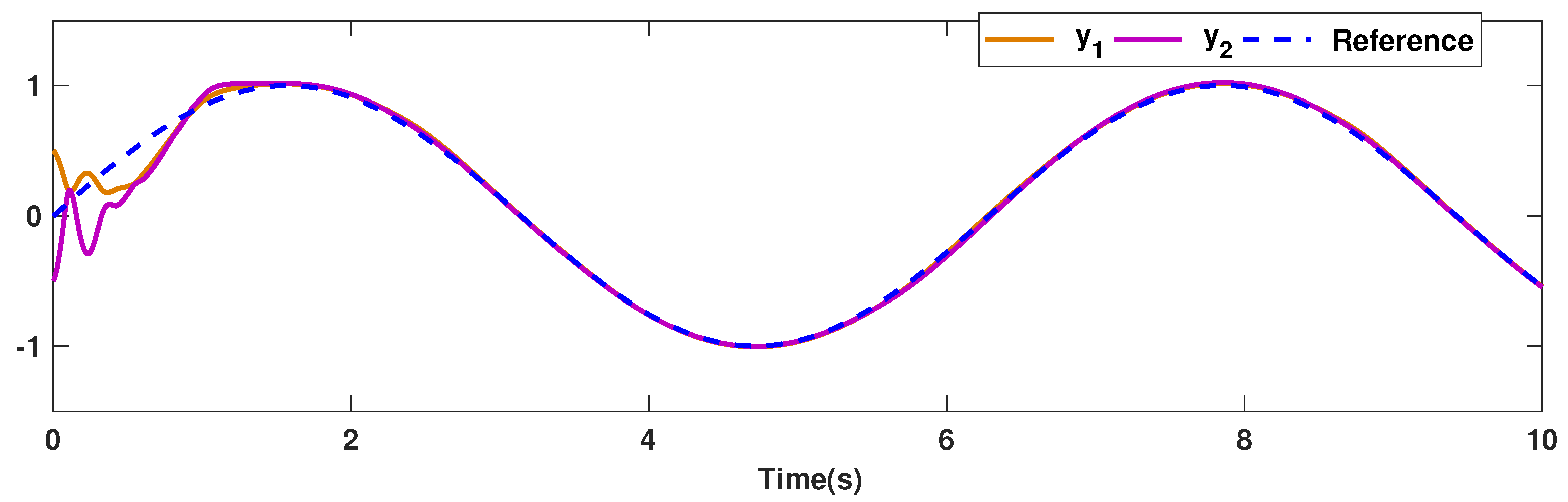
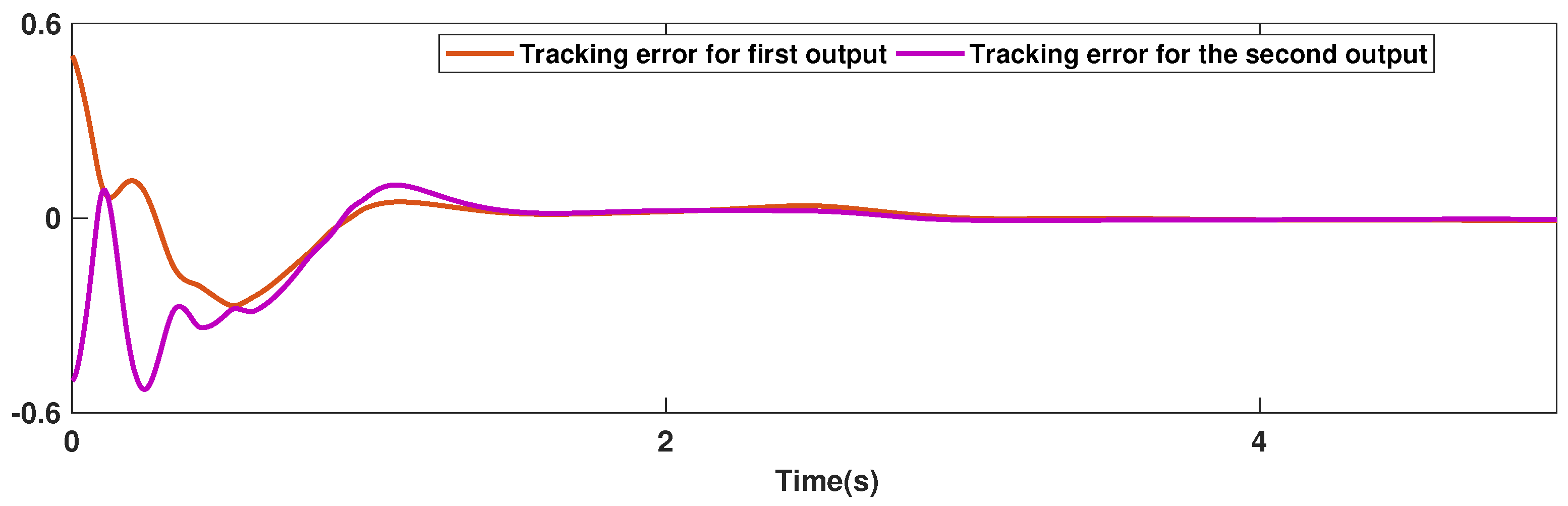
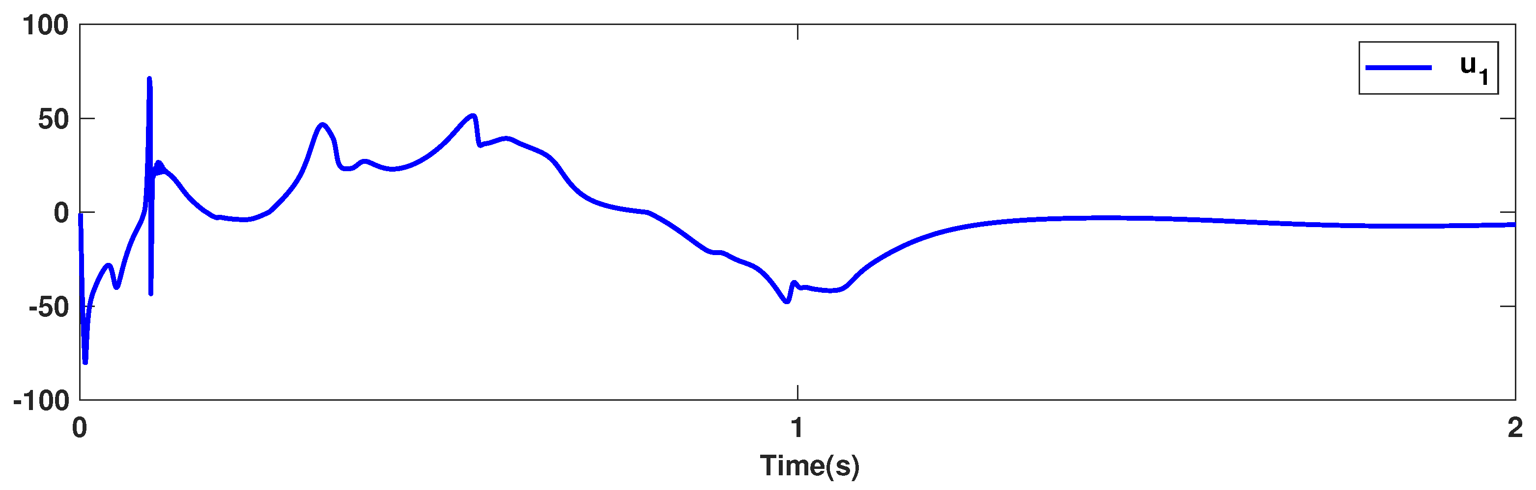
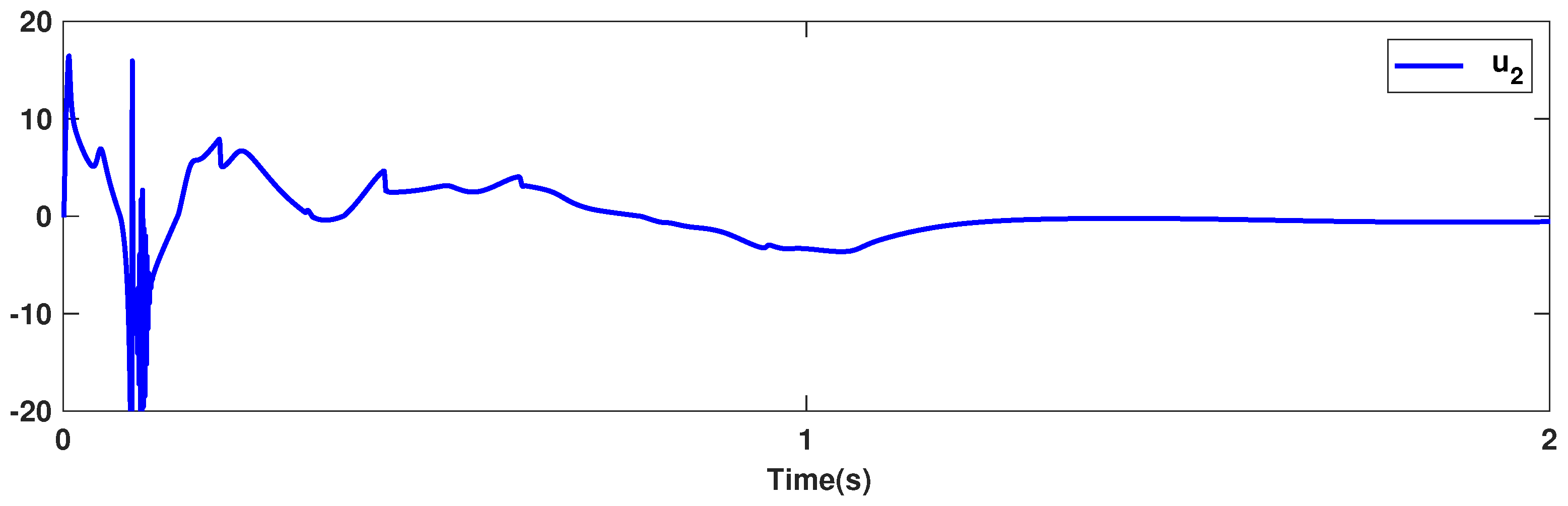
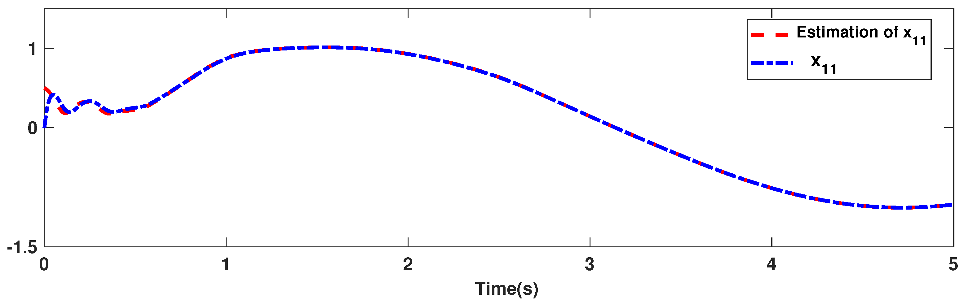
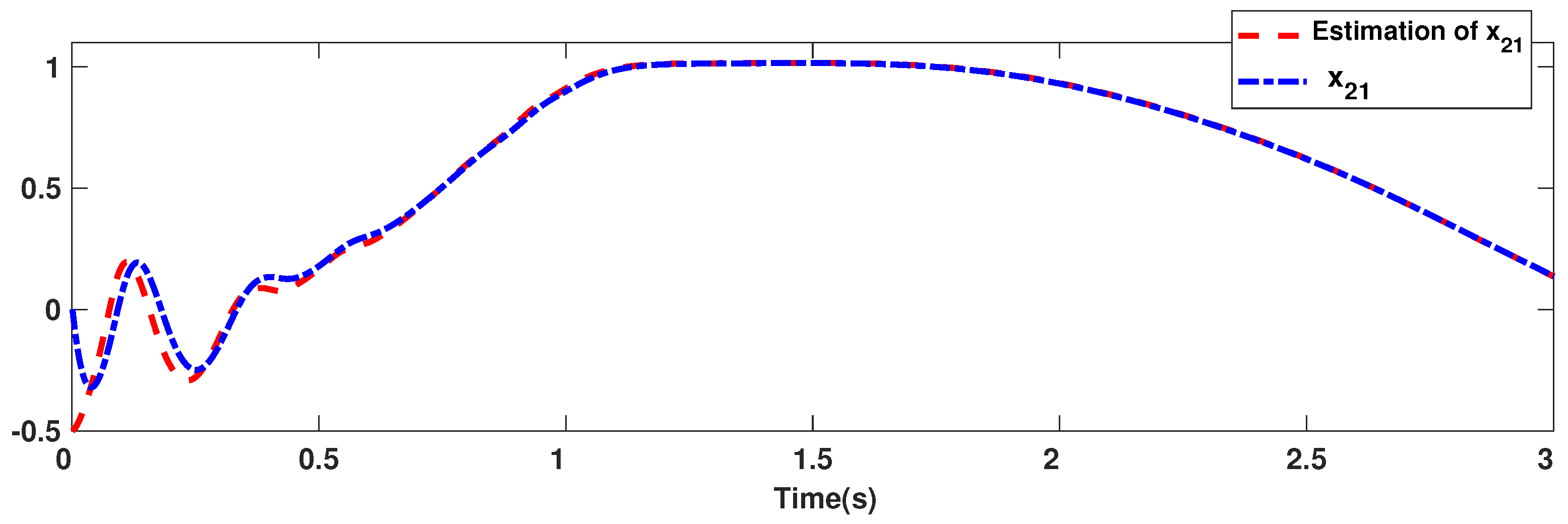
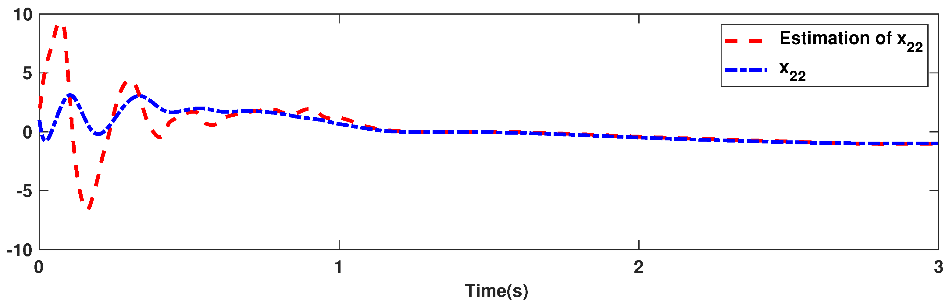
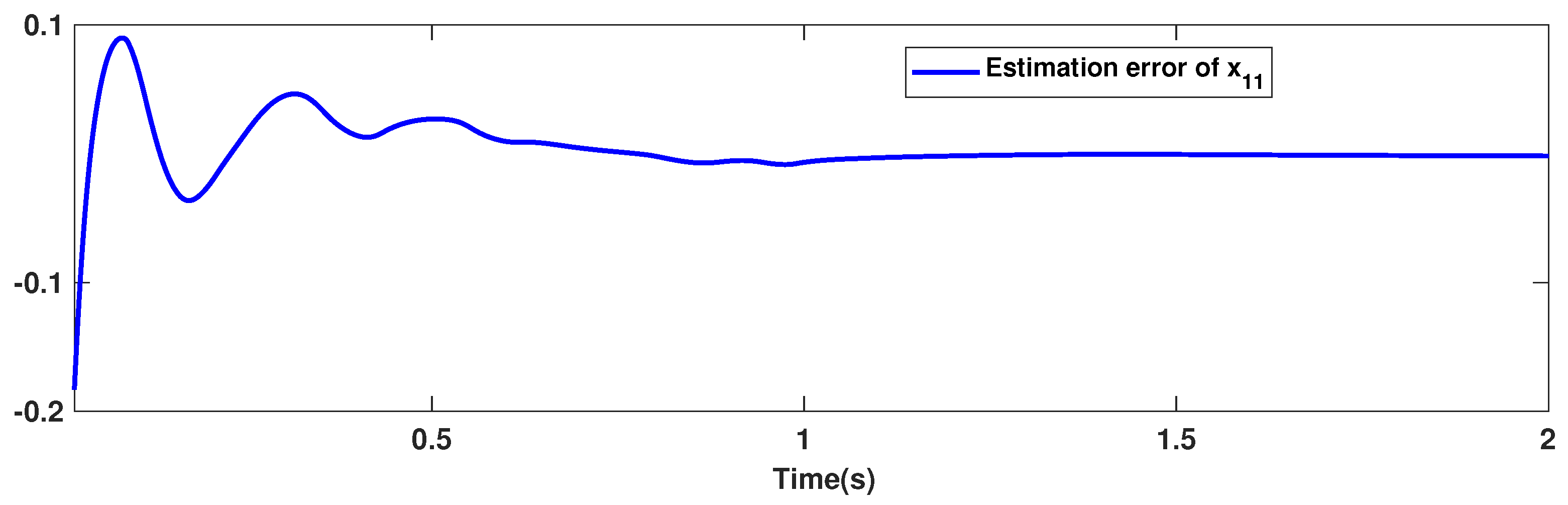
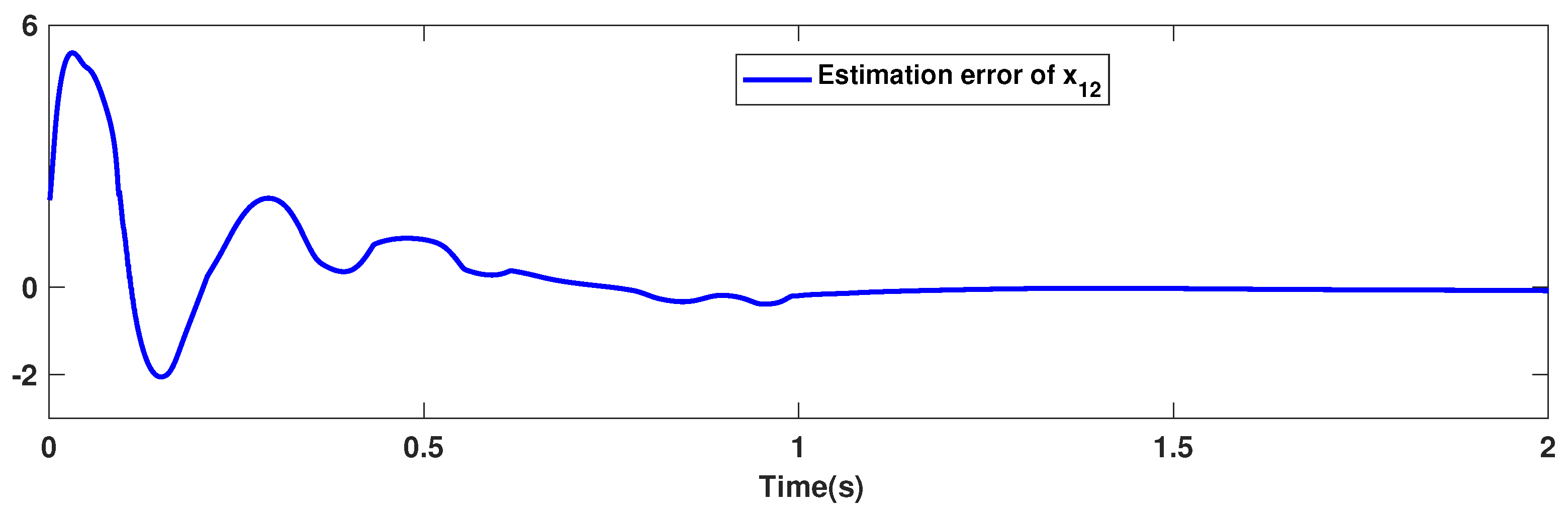
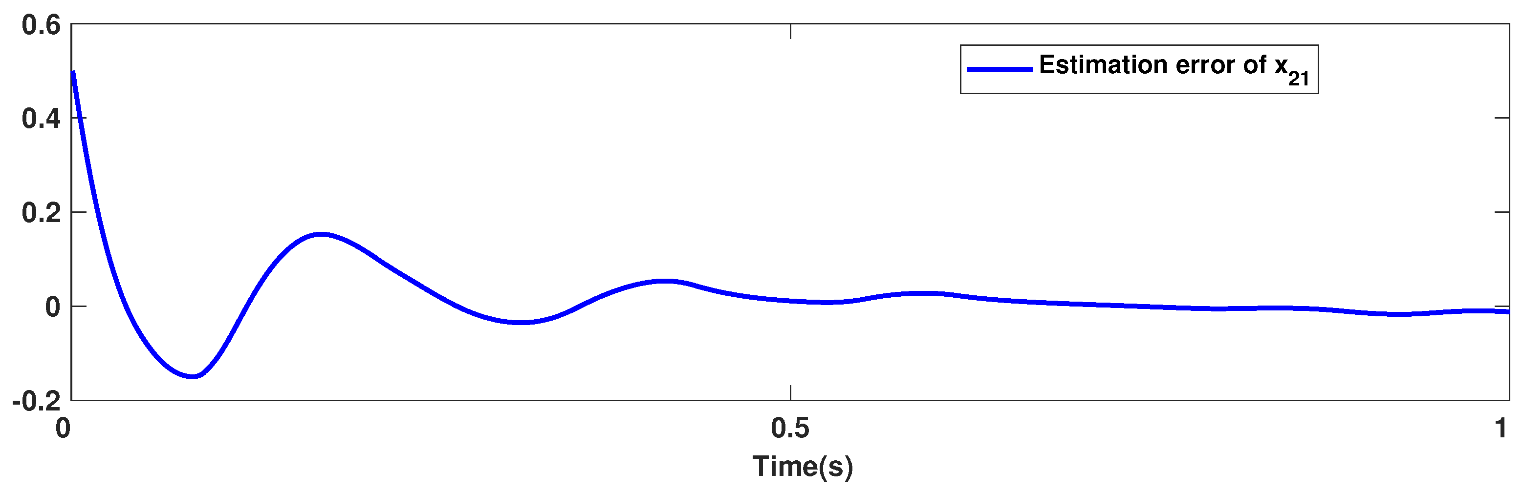
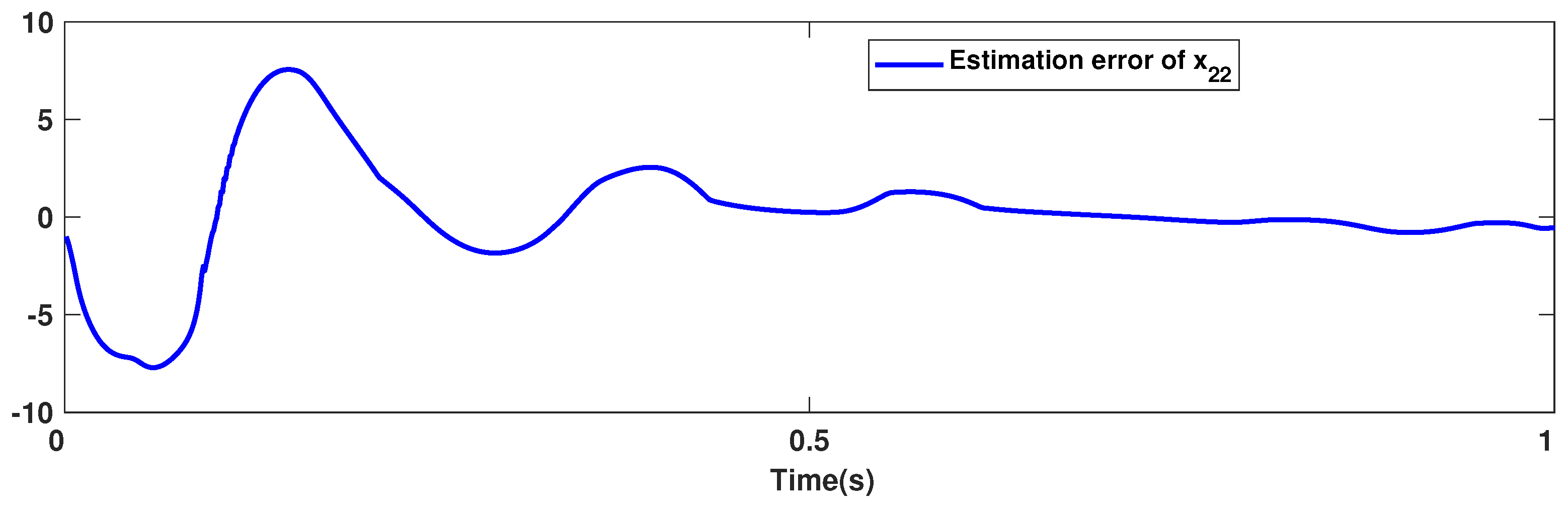
The trajectories of output are depicted in Figure 4. The outputs and approach the reference signals in a short time. The corresponding errors of and are given in Figure 5. The errors reach zero, which demonstrates the good ability of the suggested controller. The control signals are given in Figure 6 and Figure 7. The trajectories in Figure 6 and Figure 7 show that the suggested approach results in implementable control signals. There are no high-frequency fluctuations in the trajectories. The estimation performance for , , , and are given in Figure 8, Figure 9, Figure 10 and Figure 11. The trajectories in Figure 8, Figure 9, Figure 10 and Figure 11 demonstrate the good efficacy of the suggested estimation approach. The suggested FLS estimates the nonlinearities well. The estimation errors are given in Figure 12, Figure 13, Figure 14 and Figure 15. The estimation errors approach zero in a short time.
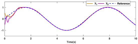
Figure 4.
Output trajectories.
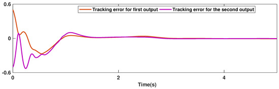
Figure 5.
Tracking trajectories.
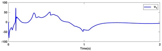
Figure 6.
Control signal .

Figure 7.
Control signal .
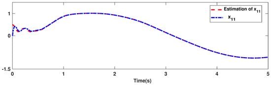
Figure 8.
Estimation accuracy of .
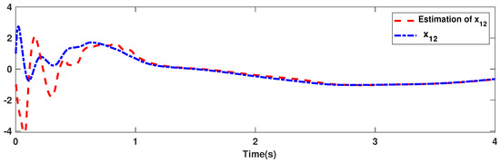
Figure 9.
Estimation accuracy of .
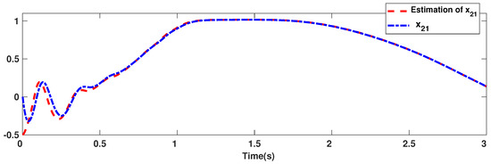
Figure 10.
Estimation accuracy of .
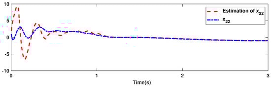
Figure 11.
Estimation accuracy of .
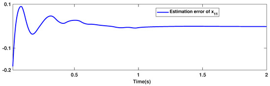
Figure 12.
Estimation error of .
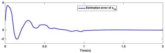
Figure 13.
Estimation error of .
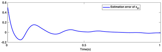
Figure 14.
Estimation error of .
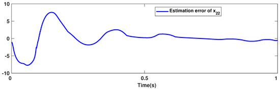
Figure 15.
Estimation error of .
T3-FLSs have better ability in a noisy environment because in T3-FLS the upper and lower bounds of uncertainties are also fuzzy numbers, not crisp values like T2-FLSs. To better show the efficiency of T3-FLSs, a comparison with T1-FLCs and T2-FLCs is given. The performance is compared in terms of the root mean square error (RMSE) in Table 1. For better comparisons, a noise with various variances is added to measured signals. It is seen that designed T3-FLC has better efficiency in a high-noise environment.

Table 1.
Performance comparison.
7. Conclusions
In this study, a new control strategy on the basis of T3-FLSs is developed for the trajectory tracking of RMs. The dynamics of RMs are unknown in the suggested approach and are estimated by T3-FLSs. The fuzzy rules of T3-FLSs are adjusted such that the robot arm tracks the desired command well. The training of T3-FLSs is carried out by the Lyapunov theorem. To ensure robustness and eliminate the perturbations and other errors, two adaptive compensators are also suggested to work in parallel with the T3-FLS-based controller. The main advantage is that the suggested controller does not depend on the dynamics RM. Additionally, it can be easily applied for various case of RMs. For examination, the designed scheme is applied to a case-study RM. In addition to the uncertain dynamics of RM, a disturbance is also considered as a sinusoid function. The results show that all states of RM are well estimated, and the tracking and estimation errors approach zero in a short time. Additionally, the suggested approach results in implementable control signals with no high-frequency fluctuations in the trajectories. The main weakness of this study is that there is no constraint of the controllers. For the future studies, the optimality of the control signals can be studied.
Author Contributions
Conceptualization, S.X., C.Z. and A.M.; methodology, S.X., C.Z. and A.M.; formal analysis, S.X., C.Z. and A.M.; writing–original draft preparation, S.X., C.Z. and A.M. All authors have read and agreed to the published version of the manuscript.
Funding
This research is financially supported by the Ministry of Science and Technology of China (Grant No. 2019YFE0112400), the Department of Science and Technology of Shandong Province (Grant No. 2021CXGC011204).
Data Availability Statement
Not applicable.
Conflicts of Interest
The authors declare no conflict of interest.
References
- Mancilla, A.; García-Valdez, M.; Castillo, O.; Merelo-Guervós, J.J. Optimal Fuzzy Controller Design for Autonomous Robot Path Tracking Using Population-Based Metaheuristics. Symmetry 2022, 14, 202. [Google Scholar] [CrossRef]
- Mancilla, A.; Castillo, O.; Garcia-Valdez, M. Optimization of Fuzzy-Control Parameters for Path Tracking of a Mobile Robot Using Distributed Genetic Algorithms. In New Perspectives on Hybrid Intelligent System Design Based on Fuzzy Logic, Neural Networks and Metaheuristics; Springer: Berlin/Heidelberg, Germany, 2022; pp. 167–177. [Google Scholar]
- Wang, J.; Yang, M.; Liang, F.; Feng, K.; Zhang, K.; Wang, Q. An algorithm for painting large objects based on a nine-axis UR5 robotic manipulator. Appl. Sci. 2022, 12, 7219. [Google Scholar] [CrossRef]
- Zhao, R.; Dai, H.; Yao, H. Liquid-metal magnetic soft robot with reprogrammable magnetization and stiffness. IEEE Robot. Autom. Lett. 2022, 7, 4535–4541. [Google Scholar] [CrossRef]
- Meng, Q.; Lai, X.; Yan, Z.; Su, C.Y.; Wu, M. Motion planning and adaptive neural tracking control of an uncertain two-link rigid–flexible manipulator with vibration amplitude constraint. IEEE Trans. Neural Netw. Learn. Syst. 2021, 33, 3814–3828. [Google Scholar] [CrossRef]
- Chen, Y.H.; Chen, Y.Y. Nonlinear Adaptive Fuzzy Control Design for Wheeled Mobile Robots with Using the Skew Symmetrical Property. Symmetry 2023, 15, 221. [Google Scholar] [CrossRef]
- Chen, Y.H.; Chen, Y.Y. Trajectory Tracking Design for a Swarm of Autonomous Mobile Robots: A Nonlinear Adaptive Optimal Approach. Mathematics 2022, 10, 3901. [Google Scholar] [CrossRef]
- Li, S.; Geng, Z. Bicriteria scheduling on an unbounded parallel-batch machine for minimizing makespan and maximum cost. Inf. Process. Lett. 2023, 180, 106343. [Google Scholar] [CrossRef]
- Wang, J.; Liang, F.; Zhou, H.; Yang, M.; Wang, Q. Analysis of Position, pose and force decoupling characteristics of a 4-UPS/1-RPS parallel grinding robot. Symmetry 2022, 14, 825. [Google Scholar] [CrossRef]
- Lai, X.; Yang, B.; Ma, B.; Liu, M.; Yin, Z.; Yin, L.; Zheng, W. An Improved Stereo Matching Algorithm Based on Joint Similarity Measure and Adaptive Weights. Appl. Sci. 2022, 13, 514. [Google Scholar] [CrossRef]
- Duan, J.; Duan, G.; Cheng, S.; Cao, S.; Wang, G. Fixed-time time-varying output formation-containment control of heterogeneous general multi-agent systems. ISA Trans. 2023. [Google Scholar] [CrossRef]
- Xu, W.; Qu, S.; Zhang, C. Fast terminal sliding mode current control with adaptive extended state disturbance observer for PMSM system. IEEE J. Emerg. Sel. Top. Power Electron. 2022, 11, 418–431. [Google Scholar] [CrossRef]
- Cuevas, F.; Castillo, O.; Cortés-Antonio, P. Generalized Type-2 Fuzzy Parameter Adaptation in the Marine Predator Algorithm for Fuzzy Controller Parameterization in Mobile Robots. Symmetry 2022, 14, 859. [Google Scholar] [CrossRef]
- Luna-Lobano, L.; Cortés-Antonio, P.; Castillo, O.; Melin, P. Analysis of P, PI, Fuzzy and Fuzzy PI Controllers for Control Position in Omnidirectional Robots. In Intuitionistic and Type-2 Fuzzy Logic Enhancements in Neural and Optimization Algorithms: Theory and Applications; Springer: Berlin/Heidelberg, Germany, 2020; pp. 339–353. [Google Scholar]
- Precup, R.E.; Preitl, S.; Petriu, E.; Bojan-Dragos, C.A.; Szedlak-Stinean, A.I.; Roman, R.C.; Hedrea, E.L. Model-based fuzzy control results for networked control systems. Rep. Mech. Eng. 2020, 1, 10–25. [Google Scholar] [CrossRef]
- Milošević, T.D.; Pamučar, D.S.; Chatterjee, P. Model for selecting a route for the transport of hazardous materials using a fuzzy logic system. Vojnoteh. Glas. Tech. Cour. 2021, 69, 355–390. [Google Scholar] [CrossRef]
- Wu, X.; Huang, Y. Adaptive fractional-order non-singular terminal sliding mode control based on fuzzy wavelet neural networks for omnidirectional mobile robot manipulator. ISA Trans. 2022, 121, 258–267. [Google Scholar] [CrossRef]
- Zhai, A.; Wang, J.; Zhang, H.; Lu, G.; Li, H. Adaptive robust synchronized control for cooperative robotic manipulators with uncertain base coordinate system. ISA Trans. 2022, 126, 134–143. [Google Scholar] [CrossRef]
- Muñoz-Vázquez, A.J.; Treesatayapun, C. Model-free discrete-time fractional fuzzy control of robotic manipulators. J. Frankl. Inst. 2022, 359, 952–966. [Google Scholar] [CrossRef]
- Zaare, S.; Soltanpour, M.R. Adaptive fuzzy global coupled nonsingular fast terminal sliding mode control of n-rigid-link elastic-joint robot manipulators in presence of uncertainties. Mech. Syst. Signal Process. 2022, 163, 108165. [Google Scholar] [CrossRef]
- Su, H.; Zhang, J.; She, Z.; Zhang, X.; Fan, K.; Zhang, X.; Liu, Q.; Ferrigno, G.; De Momi, E. Incorporating model predictive control with fuzzy approximation for robot manipulation under remote center of motion constraint. Complex Intell. Syst. 2022, 8, 2883–2895. [Google Scholar] [CrossRef]
- Zhou, J.; Liu, E.; Tian, X.; Li, Z. Adaptive Fuzzy Backstepping Control Based on Dynamic Surface Control for Uncertain Robotic Manipulator. IEEE Access 2022, 10, 23333–23341. [Google Scholar] [CrossRef]
- Song, Z.; Yi, J.; Zhao, D.; Li, X. A computed torque controller for uncertain robotic manipulator systems: Fuzzy approach. Fuzzy Sets Syst. 2005, 154, 208–226. [Google Scholar] [CrossRef]
- Dawson, D.; Qu, Z.; Lewis, F. Hybrid adaptive-robust control for a robot manipulator. Int. J. Adapt. Control Signal Process. 1992, 6, 537–545. [Google Scholar] [CrossRef]
- Keighobadi, J.; Fateh, M.M. Adaptive robust tracking control based on backstepping method for uncertain robotic manipulators including motor dynamics. Int. J. Ind. Electron. Control Optim. 2021, 4, 13–22. [Google Scholar]
- Fateh, M.M. Variable structure slip control for grasping objects. In Proceedings of the 2nd WSEAS International Conference on Dynamical Systems and Control, Bucharest, Romania, 16–18 October 2006; pp. 64–67. [Google Scholar]
- Dai, J.; Zhang, Y.; Deng, H. Novel Voltage-Based Weighted Hybrid Force/Position Control for Redundant Robot Manipulators. Electronics 2022, 11, 179. [Google Scholar] [CrossRef]
- Ding, S.; Peng, L.; Wen, J.; Zhao, H.; Liu, R. Trajectory tracking control of underactuated tendon-driven truss-like manipulator based on type-1 and interval type-2 fuzzy logic approach. Int. J. Intell. Syst. 2022, 37, 3736–3771. [Google Scholar] [CrossRef]
- Xu, X.; Shaker, A.; Salem, M.S. Automatic Control of a Mobile Manipulator Robot Based on Type-2 Fuzzy Sliding Mode Technique. Mathematics 2022, 10, 3773. [Google Scholar] [CrossRef]
- Aghaseyedabdollah, M.; Abedi, M.; Pourgholi, M. Supervisory adaptive interval type-2 fuzzy sliding mode control for planar cable-driven parallel robots using Grasshopper optimization. Iran. J. Fuzzy Syst. 2022, 19, 111–129. [Google Scholar]
- Zou, X.; Zhao, T.; Dian, S. Finite-time adaptive interval type-2 fuzzy tracking control for Mecanum-wheel mobile robots. Int. J. Fuzzy Syst. 2022, 24, 1570–1585. [Google Scholar] [CrossRef]
- Li, D.; Yu, H.; Tee, K.P.; Wu, Y.; Ge, S.S.; Lee, T.H. On time-synchronized stability and control. IEEE Trans. Syst. Man Cybern. Syst. 2021, 52, 2450–2463. [Google Scholar] [CrossRef]


Disclaimer/Publisher’s Note: The statements, opinions and data contained in all publications are solely those of the individual author(s) and contributor(s) and not of MDPI and/or the editor(s). MDPI and/or the editor(s) disclaim responsibility for any injury to people or property resulting from any ideas, methods, instructions or products referred to in the content. |
© 2023 by the authors. Licensee MDPI, Basel, Switzerland. This article is an open access article distributed under the terms and conditions of the Creative Commons Attribution (CC BY) license (https://creativecommons.org/licenses/by/4.0/).