Epidemiological Analysis of Symmetry in Transmission of the Ebola Virus with Power Law Kernel

Abstract

This study presents a mathematical model of non-integer order through the fractal fractional Caputo operator to determine the development of Ebola virus infections. To construct the model and conduct analysis, all Ebola virus cases are taken as incidence data. A symmetric approach is utilized for qualitative and quantitative analysis of the fractional order model. Additionally, stability is evaluated, along with the local and global effects of the virus that causes Ebola. Using the fractional order model of Ebola virus infections, the existence and uniqueness of solutions, as well the posedness and biological viability and disease free equilibrium points are confirmed. Many applications of fractional operators in modern mathematics exist, including the intricate and important study of symmetrical systems. Symmetry analysis is a powerful tool that enables the creation of numerical solutions for a given fractional differential equation very methodically. For this, we compare the results with the Caputo derivative operator to understand the dynamic behavior of the disease. The simulation demonstrates how all classes have convergent characteristics and maintain their places over time, reflecting the true behavior of Ebola virus infection. Power law kernel with the two step polynomial Newton method were used. This model seems to be quite strong and capable of reproducing the issue’s anticipated theoretical conditions.

1. Introduction

The deadly EVD (Ebola virus disease), which was initially identified in Africa, is a condition that only sometimes breaks out. EVD affects both nonhuman primates and people (such as monkeys, gorillas and chimpanzees). The initial discovery of the Ebola virus was in 1976 in the Democratic Republic of the Congo, close to the Ebola River. Since then, the virus has occasionally been responsible for epidemics in various African nations [1,2]. The precise origin of the Ebola virus is unknown to scientists. A straightforward mathematical model depicting the 2014 Ebola outbreak in Liberia was investigated by Rachah et al. [3]. The mathematical model was subsequently validated using computer simulations and historical data from the WHO. They also created a brand new mathematical model that takes immunisation of people into account. By comparing the classical and fractional SEIR epidemic Ebola virus models with real data from reports released by the World Health Organization from 27 March 2014, Area et al. [4] carried out a comparative analysis. A comparison of two mathematical models used to describe the continuous transmission of the Ebola virus in West Africa was conducted by Rachah and Torres [5]. They used two models to determine the best Ebola control and looked at numerical simulations to better predict how the virus will spread and how to manage it. They specifically looked at instances in which the two models yielded comparable outcomes.

The monograph on which A.A. Kilbas worked presents the most recent and up-to-date study on fractional and fractional integro-differential equations, employing a wide range of potentially useful fractional calculus operators. The calculus of integrals and derivatives of any arbitrary real or complex order was addressed by fractional calculus and its applications and the work was continued by Zhang [6]. In many fields of science and engineering where nonlocality plays an important role in fractional calculus, numerous models still need to be suggested, investigated and put into practice. There are still a lot of non-local phenomena that have not been explored and are only waiting to be discovered, despite the fact that many amazing findings have already been documented by researchers in significant monographs and review papers [7]. While Ali Akgul worked on Atangana Baleanu developed a derivative with fractional order to locate the crucial questions. The Atangana–Baleanu problem’s fractional derivative, as well as a new approach for researching fractional differential equations, are covered in [8]. The main goal of Akgul’s research is to solve linear and nonlinear fractional differential equations using the Mittag–Leffler kernel. A precise numerical strategy was created to address this problem. The theoretical conclusions were supported by two experiments [9]. Ford et al. [10] saught to understand the derivatives in the Caputo sense. Before examining how the solutions connect to the existing information, the existence and uniqueness of the solutions were first explored analytically. Baleanu et al. [11] adapted and tweaked the method to solve a large class of partial differential equations of fractional order. We demonstrated the approach’s value by applying it to solve a model fractional problem.

According to the report in 1976, the region of Africa had a wide spread of virus name as Ebola. The Ebola virus starts from a rural area of West Africa areas and spread over the urban area within a week, also within a month it becomes a global epidemic. Baleanu et al. [12] proposed a novel fractional derivative with a non-local and non-singular kernel. We spoke about some of the positive traits of the new derivative and applied it to solve the fractional heat transfer model. Atangana and Goufo [13] originally utilized the Ebola virus model with the classical derivative and then modified it with the beta derivative to create a generalised version. They thoroughly investigated the endemic equilibrium locations using the Jacobian approach to determine the corresponding Eigenvalues. As a consequence, they created the model by iteratively numerically addressing the problem. These answers were discovered in terms of beta and time. Using the Atangana–Baleanu fractional derivative and integral operator, Koca [14] assessed the existence and uniqueness of the solutions for the Ebola disease transmission model. Latha et al. in [15] proposed a fractional-order Ebola virus epidemic model with heterogeneous complex networks with a delayed immune response. The term "time delay" is used to describe cytotoxic T lymphocytes (CTLs). Several requirements for the model’s stability are given based on the fractional Laplace transform. Singh [16,17] undertook some studies on certain numerical solutions for mathematical models. Dokuyucu et al. [18] studied the modelling of cancer therapy using the Caputo–Fabrizio fractional derivative operator in their article. They looked into whether an answer existed. They also explored the solution’s uniqueness and determined the circumstances in which the model offers a unique answer based on research by Hasan et al. [19] a number of fractional parameters were also used to analyse the deterministic mathematical model of the Omicron effect. The Ebola virus is a highly infectious illness that, according to Farman et al. [20], has the capacity to infect the whole population, depending on the dynamics of the community and the individuals. Due to a description of the recollection and hereditary properties in [21,22,23], ordinary integer order can hinder understanding of the explanation of real-world situations, but fractional order, which requires including and transecting differentiation with the use of fractional calculus, can also help in the modelling of genuine occurrences.

The remaining portions of this research document are as follows: A thorough introduction to the proposed model is provided in Section 1, along with descriptions of some other important discoveries from the other work. Several basic fractional order derivatives contained in Section 2 are useful in resolving the epidemiological model. An extended version of the model and an evaluation of the preliminary model description may be found in Section 3, along with the proposed model’s study of well-posedness. In Section 4, a qualitative analysis of the the suggested model is given, along with the study of disease-free equilibrium, positivity of the proposed model with nonlocal operators, invariant region, existence, and uniqueness is discussed. In Section 5, an analysis of stability of the proposed scheme, such as stability of UH (Ulam–Hyres) is given. The numerical simulations and a discussion is given in Section 7. In Section 8, the conclusion is presented.

2. Fundamental Fractional Operator Concepts

In [24], we found a number of significant and practical nonlinear dynamics and modern calculus results.

Definition 1. 

If $\psi \left(t\right)$ is continuous, it is continuous and differentiable in the interval $]a,b[$, then its fractal fractional derivative of order $\upsilon \in (0,1)$ with a Caputo-type kernel is provided by

$${}^{\mathfrak{C}}{\mathbb{D}}_t^{\upsilon }\psi \left(t\right)=\frac{1}{\Gamma (\xi -\upsilon )}{\int }_0^t\frac{{\psi }^{\xi }\left(\rho \right)}{{(t-\rho )}^{\upsilon -\xi +1}}d\rho ,$$

(1)

where $\xi =\left[\upsilon \right]+1$, $\xi <\upsilon +1$ and $\left[\upsilon \right]$ represent the integer parts of υ.

Definition 2. 

The fractal fractional integral of order $\upsilon \in (0,1)$ with a Caputo-type kernel is given by

$${}^{\mathfrak{C}}{\mathbb{I}}_t^{\upsilon }\psi \left(t\right)=\frac{1}{\Gamma \left(\upsilon \right)}{\int }_0^t{(t-\rho )}^{\upsilon -1}d\rho ,$$

(2)

if the interval $]a,b[$ is continuous for $\psi \left(t\right)$.

Definition 3. 

Let ${\varphi }^{☆}$ be the equilibrium point in the Caputo fractional dynamical system if the interval $]a,b[$ is continuous for $\psi \left(t\right)$

$$\begin{array}{ccc}\hfill {}^{\mathfrak{C}}{\mathbb{D}}_t^{\upsilon }\psi \left(t\right)=f(t,\varphi \left(t\right)),& \hfill & \hfill \upsilon \in (0,1),\end{array}$$

(3)

if $f(t,{\varphi }^{☆}\left(t\right))=0$.

3. Fractional-Order Model of Ebola with Treatment

We offer a deterministic model to better comprehend the dynamics of Ebola virus transmission. The causes and recurrence of epidemics are being investigated through simulations by researchers. Let us look at some of the key aspects of the compartmental mathematical epidemic model that Rama et al. [25] devised to explain viral transmission.

The epidemic Ebola virus treatment model is described by a set of nonlinear ordinary differential equations as follows

$$\left\{\begin{array}{c}{}^{\mathfrak{C}}{\mathbb{D}}_{0,t}^{{\upsilon }_1,{\upsilon }_2}S\left(t\right)=\Lambda -\left({\beta }_{I}I+{\beta }_{H}H+{\beta }_{D}D\right)S-(\tau +\mu )S,\hfill \\ {}^{\mathfrak{C}}{\mathbb{D}}_{0,t}^{{\upsilon }_1,{\upsilon }_2}E\left(t\right)=S\left({\beta }_{I}I+{\beta }_{H}H+{\beta }_{D}D\right)-(\mu +\tau +\delta )E,\hfill \\ {}^{\mathfrak{C}}{\mathbb{D}}_{0,t}^{{\upsilon }_1,{\upsilon }_2}I\left(t\right)=\delta E-(\mu +\gamma )I,\hfill \\ {}^{\mathfrak{C}}{\mathbb{D}}_{0,t}^{{\upsilon }_1,{\upsilon }_2}H\left(t\right)=\gamma I-(\mu +\lambda +\alpha )H,\hfill \\ {}^{\mathfrak{C}}{\mathbb{D}}_{0,t}^{{\upsilon }_1,{\upsilon }_2}R\left(t\right)=\alpha H-(\mu +\tau )R,\hfill \\ {}^{\mathfrak{C}}{\mathbb{D}}_{0,t}^{{\upsilon }_1,{\upsilon }_2}D\left(t\right)=\lambda H-\theta D.\hfill \end{array}\right.$$

(4)

where the initial conditions are

$$S\left(0\right)=S^0\ge 0,H\left(0\right)=H^0\ge 0,E\left(0\right)=E^0\ge 0,I\left(0\right)=I^0\ge 0,R\left(0\right)=R^0\ge 0,D\left(0\right)=D^0\ge 0.$$

(5)

3.1. Model Description

The population is divided into four divisions according to our mathematical model, which is displayed in Table 1.

Table 1. The classes of the proposed model are described.

$S\left(t\right)$	Group of vulnerable individuals
$E\left(t\right)$	Group of infected people
$I\left(t\right)$	Group of contagion carriers
$H\left(t\right)$	Class of hospitalized people
$D\left(t\right)$	Class of dead people
$R\left(t\right)$	Class of recovered people

3.2. Model Assumptions

The following assumptions were made in the model

1.

People who have not been exposed to the illness pathogen are placed in the susceptible class $S\left(t\right)$.

2.

Those that reside in this class $I\left(t\right)$ have the disease pathogen but do not exhibit overt clinical symptoms. They are not yet able to spread infection. This is the incubation phase. People then proceed to the infectious class at the conclusion of this phase.

3.

People begin exhibiting clinical symptoms and potentially spread an infection to others $E\left(t\right)$. Authorities place infectious patients under sanitary care after the infectious period, which is the average amount of time a person spends in this class and then classify them as hospitalized.

4.

Although they are receiving treatment, the individuals in this class $H\left(t\right)$ are still contagious. After the hospital stay, patients have two options: heal (and move into the recovered class) or pass away (dead class). We specifically state that there are no hospitalized patients who are no longer able to spread disease in class H. They are classified as described below as “recovered”.

5.

People who have died from the disease but have not yet been buried $D\left(t\right)$ are still contagious to others through touch. The body is interred after a predetermined amount of time.

6.

This class $R\left(t\right)$ consists of survivors of the virus. In this class, people are naturally immune to the disease-causing agent and stop being contagious.

The full list of parameters for the proposed model is presented in Table 2.

Table 2. The suggested model parameters.

$\Lambda$	Rate of recruitment of individuals in state S
$\mu$	The death rate
${\beta }_I$	The effective contact rates for diseases among those in compartment I
${\beta }_H$	People in class H’s rates of effective disease contact
${\beta }_D$	The effective contact rates for diseases among those in compartment D
$\delta$	Rate of change from compartment E to I
$\gamma$	Rate of change from compartment E to compartment I
$\lambda$	The result of the sickness mortality rate multiplied by the compartment H to compartment D transition rate
$\alpha$	The percentage of illnesses that survive multiplied by the transition rate from condition H to compartment R
$\theta$	The percentage of Ebola victims buried
$\tau$	The daily percentage of persons departing the nation in states S, E, and R

Thus, the total population is established by

$$\mathbb{N}\left(t\right)=S\left(t\right)+H\left(t\right)+E\left(t\right)+I\left(t\right)+R\left(t\right)+D\left(t\right).$$

(6)

4. Well Posedness of the Model

The time period and region where the roots to our proposed system makes cultural sense are examined in this section. We have already proven that all solutions and suggested parameters are positive for all t. We know that for everyone, $t>0$.

$${}^{\mathfrak{C}}{\mathbb{D}}_{0,t}^{{\upsilon }_1,{\upsilon }_2}\mathbb{N}\left(t\right)=-\mu \mathbb{N}\left(t\right)+\Lambda .$$

(7)

We desire the function $\mathbb{N}\left(t\right)$ to be an increasing function, ${}^{\mathfrak{C}}{\mathbb{D}}_{0,t}^{{\upsilon }_1,{\upsilon }_2}\mathbb{N}\left(t\right)>0$

$${}^{\mathfrak{C}}{\mathbb{D}}_{0,t}^{{\upsilon }_1,{\upsilon }_2}\mathbb{N}\left(t\right)\ge \mathbb{N}\left(t\right)<\frac{\Lambda }{\mu }.$$

(8)

The level of threshold population is how the literature describes the aforementioned disparity. This leads us to the conclusion that the recognised set of solutions for the suggested model should be restricted to

$$\mathsf{Y}=\left\{(S,E,I,H,R,D)\in R_{+}^6:S+E+H+I+R+D=\mathbb{N}<\frac{\Lambda }{\mu }\right\}.$$

(9)

The $+ve$ cone of $R_{+}^6$ in this instance also contains its faces in the smaller faces. In the interest of reality, we rule out the possibility that the host population ultimately reaches its carrying capacity if ${}^{\mathfrak{C}}{\mathbb{D}}_{0,t}^{{\upsilon }_1,{\upsilon }_2}\mathbb{N}\left(t\right)\ge 0$.

5. Qualitative Analysis of the Proposed Model

To learn more about the characteristics of the Ebola virus and to comprehend the variables that affect how the virus spreads.

5.1. Equilibrium Point of the Model

Setting the left hand side of system (4), we obtain an equilibrium point that is $P^{☆}=\{S^{☆},E^{☆},I^{☆},H^{☆},R^{☆},D^{☆}\}$, where

$$S^{☆}=\frac{{\Xi }_1}{{\Xi }_2}.$$

(10)

$$\begin{array}{cc}\hfill {\Xi }_1=& \theta (\alpha \delta \gamma +\alpha \delta \mu +\alpha \gamma \mu +\alpha \gamma \tau +\alpha {\mu }^2+\alpha \mu \tau +\delta \gamma \lambda +\delta \gamma \mu +\delta \lambda \mu +\delta {\mu }^2+\gamma \lambda \mu \hfill \\ & +\gamma \lambda \tau +\gamma {\mu }^2+\gamma \mu \tau +\lambda {\mu }^2+\lambda \mu \tau +{\mu }^3+{\mu }^2\tau ).\hfill \end{array}$$

$$\begin{array}{c}\hfill {\Xi }_2=\delta (\alpha \theta {\beta }_I+\gamma \lambda {\beta }_D+\gamma \theta {\beta }_H+\lambda \theta {\beta }_I+\mu \theta {\beta }_I).\end{array}$$

$$E^{☆}=\frac{{\Xi }_3}{{\Xi }_4}.$$

(11)

$$\begin{array}{cc}\hfill {\Xi }_3=& \Lambda \alpha \delta \theta {\beta }_I+\Lambda \delta \gamma \lambda {\beta }_D+\Lambda \delta \gamma \theta {\beta }_H+\Lambda \delta \lambda \theta {\beta }_I+\Lambda \delta \mu \theta {\beta }_I-\alpha \delta \gamma \mu \theta -\alpha \delta \gamma \tau \theta -\alpha \delta {\mu }^2\theta \hfill \\ & -\alpha \delta \mu \tau \theta -\alpha \gamma {\mu }^2\theta -2\alpha \gamma \mu \tau \theta -\alpha \gamma {\tau }^2\theta -\alpha {\mu }^3\theta -2\alpha {\mu }^2\tau \theta -\alpha \mu {\tau }^2\theta -\delta \gamma \lambda \mu \theta \hfill \\ & -\delta \gamma \lambda \tau \theta -\delta \gamma {\mu }^2\theta -\delta \gamma \mu \tau \theta -\delta \lambda {\mu }^2\theta -\delta \lambda \mu \tau \theta -\delta {\mu }^3\theta -\delta {\mu }^2\tau \theta -\gamma \lambda {\mu }^2\theta \hfill \\ & -2\gamma \lambda \mu \tau \theta -\gamma \lambda {\tau }^2\theta -\gamma {\mu }^3\theta -2\gamma {\mu }^2\tau \theta -\gamma \mu {\tau }^2\theta -\lambda {\mu }^3\theta -2\lambda {\mu }^2\tau \theta -\lambda \mu {\tau }^2\theta -{\mu }^4\theta \hfill \\ & -2{\mu }^3\tau \theta -{\mu }^2{\tau }^2\theta .\hfill \end{array}$$

$$\begin{array}{cc}\hfill {\Xi }_4=& \delta (\alpha \delta \theta {\beta }_I+\alpha \mu \theta {\beta }_I+\alpha \tau \theta {\beta }_I+\delta \gamma \lambda {\beta }_D+\delta \gamma \theta {\beta }_H+\delta \lambda \theta {\beta }_I+\delta \mu \theta {\beta }_I+\gamma \lambda \mu {\beta }_D\hfill \\ & +\gamma \lambda \tau {\beta }_D+\gamma \mu \theta {\beta }_H+\gamma \tau \theta {\beta }_H+\lambda \mu \theta {\beta }_I+\lambda \tau \theta {\beta }_I+{\mu }^2\theta {\beta }_I+\mu \tau \theta {\beta }_I).\hfill \end{array}$$

$$I^{☆}=\frac{{\Xi }_5}{{\Xi }_6}.$$

(12)

$$\begin{array}{cc}\hfill {\Xi }_5=& \Lambda \alpha \delta \theta {\beta }_I+\Lambda \delta \gamma \lambda {\beta }_D+\Lambda \delta \gamma \theta {\beta }_H+\Lambda \delta \lambda \theta {\beta }_I+\Lambda \delta \mu \theta {\beta }_I-\alpha \delta \gamma \mu \theta -\alpha \delta \gamma \tau \theta -\alpha \delta {\mu }^2\theta \hfill \\ & -\alpha \delta \mu \tau \theta -\alpha \gamma {\mu }^2\theta -2\alpha \gamma \mu \tau \theta -\alpha \gamma {\tau }^2\theta -\alpha {\mu }^3\theta -2\alpha {\mu }^2\tau \theta -\alpha \mu {\tau }^2\theta -\delta \gamma \lambda \mu \theta \hfill \\ & -\delta \gamma \lambda \tau \theta -\delta \gamma {\mu }^2\theta -\delta \gamma \mu \tau \theta -\delta \lambda {\mu }^2\theta -\delta \lambda \mu \tau \theta -\delta {\mu }^3\theta -\delta {\mu }^2\tau \theta -\gamma \lambda {\mu }^2\theta \hfill \\ & -2\gamma \lambda \mu \tau \theta -\gamma \lambda {\tau }^2\theta -\gamma {\mu }^3\theta -2\gamma {\mu }^2\tau \theta -\gamma \mu {\tau }^2\theta -\lambda {\mu }^3\theta -2\lambda {\mu }^2\tau \theta -\lambda \mu {\tau }^2\theta -{\mu }^4\theta \hfill \\ & -2{\mu }^3\tau \theta -{\mu }^2{\tau }^2\theta .\hfill \end{array}$$

$$\begin{array}{cc}\hfill {\Xi }_6=& \alpha \delta \gamma \theta {\beta }_I+\alpha \delta \mu \theta {\beta }_I+\alpha \gamma \mu \theta {\beta }_I+\alpha \gamma \tau \theta {\beta }_I+\alpha {\mu }^2\theta {\beta }_I+\alpha \mu \tau \theta {\beta }_I+\delta {\gamma }^2\lambda {\beta }_D+\delta {\gamma }^2\theta {\beta }_H\hfill \\ & +\delta \gamma \lambda \mu {\beta }_D+\delta \gamma \lambda \theta {\beta }_I+\delta \gamma \mu \theta {\beta }_I+\delta \gamma \mu \theta {\beta }_H+\delta \lambda \mu \theta {\beta }_I+\delta {\mu }^2\theta {\beta }_I+{\gamma }^2\lambda \mu {\beta }_D+{\gamma }^2\lambda \tau {\beta }_D\hfill \\ & +{\gamma }^2\mu \theta {\beta }_H+{\gamma }^2\tau \theta {\beta }_H+\gamma \lambda {\mu }^2{\beta }_D+\gamma \lambda \mu \tau {\beta }_D+\gamma \lambda \mu \theta {\beta }_I+\gamma \lambda \tau \theta {\beta }_I+\gamma {\mu }^2\theta {\beta }_I+\gamma {\mu }^2\theta {\beta }_H\hfill \\ & +\gamma \mu \tau \theta {\beta }_I+\gamma \mu \tau \theta {\beta }_H+\lambda {\mu }^2\theta {\beta }_I+\lambda \mu \tau \theta {\beta }_I+{\mu }^3\theta {\beta }_I+{\mu }^2\tau \theta {\beta }_I.\hfill \end{array}$$

$$H^{☆}=\frac{{\Xi }_7}{{\Xi }_8}.$$

(13)

$$\begin{array}{cc}\hfill {\Xi }_7=& \gamma (\Lambda \alpha \delta \theta {\beta }_I+\Lambda \delta \gamma \lambda {\beta }_D+\Lambda \delta \gamma \theta {\beta }_H+\Lambda \delta \lambda \theta {\beta }_I+\Lambda \delta \mu \theta {\beta }_I-\alpha \delta \gamma \mu \theta -\alpha \delta \gamma \tau \theta -\alpha \delta {\mu }^2\theta \hfill \\ & -\alpha \delta \mu \tau \theta -\alpha \gamma {\mu }^2\theta -2\alpha \gamma \mu \tau \theta -\alpha \gamma {\tau }^2\theta -\alpha {\mu }^3\theta -2\alpha {\mu }^2\tau \theta -\alpha \mu {\tau }^2\theta -\delta \gamma \lambda \mu \theta -\delta \gamma \lambda \tau \theta \hfill \\ & -\delta \gamma {\mu }^2\theta -\delta \gamma \mu \tau \theta -\delta \lambda {\mu }^2\theta -\delta \lambda \mu \tau \theta -\delta {\mu }^3\theta -\delta {\mu }^2\tau \theta -\gamma \lambda {\mu }^2\theta -2\gamma \lambda \mu \tau \theta -\gamma \lambda {\tau }^2\theta \hfill \\ & -\gamma {\mu }^3\theta -2\gamma {\mu }^2\tau \theta -\gamma \mu {\tau }^2\theta -\lambda {\mu }^3\theta -2\lambda {\mu }^2\tau \theta -\lambda \mu {\tau }^2\theta -{\mu }^4\theta -2{\mu }^3\tau \theta -{\mu }^2{\tau }^2\theta ).\hfill \end{array}$$

$$\begin{array}{cc}\hfill {\Xi }_8=& {\alpha }^2\delta \gamma \theta {\beta }_I+{\alpha }^2\delta \mu \theta {\beta }_I+{\alpha }^2\gamma \mu \theta {\beta }_I+{\alpha }^2\gamma \tau \theta {\beta }_I+{\alpha }^2{\mu }^2\theta {\beta }_I+{\alpha }^2\mu \tau \theta {\beta }_I+\alpha \delta {\gamma }^2\lambda {\beta }_D\hfill \\ & +\alpha \delta {\gamma }^2\theta {\beta }_H+\alpha \delta \gamma \lambda \mu {\beta }_D+2\alpha \delta \gamma \lambda \theta {\beta }_I+2\alpha \delta \gamma \mu \theta {\beta }_I+\alpha \delta \gamma \mu \theta {\beta }_H+2\alpha \delta \lambda \mu \theta {\beta }_I\hfill \\ & +2\alpha \delta {\mu }^2\theta {\beta }_I+\alpha {\gamma }^2\lambda \mu {\beta }_D+\alpha {\gamma }^2\lambda \tau {\beta }_D+\alpha {\gamma }^2\mu \theta {\beta }_H+\alpha {\gamma }^2\tau \theta {\beta }_H+\alpha \gamma \lambda {\mu }^2{\beta }_D\hfill \\ & +\alpha \gamma \lambda \mu \tau {\beta }_D+2\alpha \gamma \lambda \mu \theta {\beta }_I+2\alpha \gamma \lambda \tau \theta {\beta }_I+2\alpha \gamma {\mu }^2\theta {\beta }_I+\alpha \gamma {\mu }^2\theta {\beta }_I+2\alpha \gamma \mu \tau \theta {\beta }_I\hfill \\ & +\alpha \gamma \mu \tau \theta {\beta }_H+2\alpha \lambda {\mu }^2\theta {\beta }_I+2\alpha \lambda \mu \tau \theta {\beta }_I+2\alpha {\mu }^3\theta {\beta }_I+2\alpha {\mu }^2\tau \theta {\beta }_I+\delta {\gamma }^2{\lambda }^2{\beta }_D\hfill \\ & +\delta {\gamma }^2\lambda \mu {\beta }_D+\delta {\gamma }^2\lambda \theta {\beta }_H+\delta {\gamma }^2\mu \theta {\beta }_H+\delta \gamma {\lambda }^2\mu {\beta }_H+\delta \gamma {\lambda }^2\theta {\beta }_I+\delta \gamma \lambda {\mu }^2{\beta }_D\hfill \\ & +2\delta \gamma \lambda \mu \theta {\beta }_I+\delta \gamma \lambda \mu \theta {\beta }_H+\delta \gamma {\mu }^2\theta {\beta }_I+\delta \gamma {\mu }^2\theta {\beta }_H+\delta {\lambda }^2\mu \theta {\beta }_I+2\delta \lambda {\mu }^2\theta {\beta }_I\hfill \\ & +\delta {\mu }^3\theta {\beta }_I+{\gamma }^2{\lambda }^2\mu {\beta }_D+{\gamma }^2{\lambda }^2\tau {\beta }_D+{\gamma }^2\lambda {\mu }^2{\beta }_D+{\gamma }^2\lambda \mu \tau {\beta }_D+{\gamma }^2\lambda \mu \theta {\beta }_H+{\gamma }^2\lambda \tau \theta {\beta }_H\hfill \\ & +{\gamma }^2{\mu }^2\theta {\beta }_H+{\gamma }^2\mu \tau \theta {\beta }_H+\gamma {\lambda }^2{\mu }^2{\beta }_D+\gamma {\lambda }^2\mu \tau {\beta }_D+\gamma {\lambda }^2\mu \theta {\beta }_I+\gamma {\lambda }^2\tau \theta {\beta }_I+\gamma \lambda {\mu }^3{\beta }_D\hfill \\ & +\gamma \lambda {\mu }^2\tau {\beta }_D+2\gamma \lambda {\mu }^2\theta {\beta }_I+\gamma \lambda {\mu }^2\theta {\beta }_H+2\gamma \lambda \mu \tau \theta {\beta }_I+\gamma \lambda \mu \tau \theta {\beta }_H+\gamma {\mu }^3\theta {\beta }_I+\gamma {\mu }^3\theta {\beta }_H\hfill \\ & +\gamma {\mu }^2\tau \theta {\beta }_I+\gamma {\mu }^2\tau \theta {\beta }_H+{\lambda }^2{\mu }^2\theta {\beta }_I+{\lambda }^2\mu \tau \theta {\beta }_I+2\lambda {\mu }^3\theta {\beta }_I+2\lambda {\mu }^2\tau \theta {\beta }_I+{\mu }^4\theta {\beta }_I+{\mu }^3\tau \theta {\beta }_I.\hfill \end{array}$$

$$R^{☆}=\frac{{\Xi }_9}{{\Xi }_{10}}.$$

(14)

$$\begin{array}{cc}\hfill {\Xi }_9=& \alpha \gamma (\Lambda \alpha \delta \theta {\beta }_I+\Lambda \delta \gamma \lambda {\beta }_D+\Lambda \delta \gamma \theta {\beta }_H+\Lambda \delta \lambda \theta {\beta }_I+\Lambda \delta \mu \theta {\beta }_I-\alpha \delta \gamma \mu \theta -\alpha \delta \gamma \tau \theta -\alpha \delta {\mu }^2\theta \hfill \\ & -\alpha \delta \mu \tau \theta -\alpha \gamma {\mu }^2\theta -2\alpha \gamma \mu \tau \theta -\alpha \gamma {\tau }^2\theta -\alpha {\mu }^3\theta -2\alpha {\mu }^2\tau \theta -\alpha \mu {\tau }^2\theta -\delta \gamma \lambda \mu \theta -\delta \gamma \lambda \tau \theta \hfill \\ & -\delta \gamma {\mu }^2\theta -\delta \gamma \mu \tau \theta -\delta \lambda {\mu }^2\theta -\delta \lambda \mu \tau \theta -\delta {\mu }^3\theta -\delta {\mu }^2\tau \theta -\gamma \lambda {\mu }^2\theta -2\gamma \lambda \mu \tau \theta -\gamma \lambda {\tau }^2\theta \hfill \\ & -\gamma {\mu }^3\theta -2\gamma {\mu }^2\tau \theta -\gamma \mu {\tau }^2\theta -\lambda {\mu }^3\theta -2\lambda {\mu }^2\tau \theta -\lambda \mu {\tau }^2\theta -{\mu }^4\theta -2{\mu }^3\tau \theta -{\mu }^2{\tau }^2\theta ).\hfill \end{array}$$

$$\begin{array}{cc}\hfill {\Xi }_{10}=& ({\alpha }^2\delta \gamma \theta {\beta }_I+{\alpha }^2\delta \mu \theta {\beta }_I+{\alpha }^2\gamma \mu \theta {\beta }_I+{\alpha }^2\gamma \tau \theta {\beta }_I+{\alpha }^2{\mu }^2\theta {\beta }_I+{\alpha }^2\mu \tau \theta {\beta }_I+\alpha \delta {\gamma }^2\lambda {\beta }_D\hfill \\ & +\alpha \delta {\gamma }^2\theta {\beta }_H+\alpha \delta \gamma \lambda \mu {\beta }_D+2\alpha \delta \gamma \lambda \theta {\beta }_I+2\alpha \delta \gamma \mu \theta {\beta }_I+\alpha \delta \gamma \mu \theta {\beta }_H+2\alpha \delta \lambda \mu \theta {\beta }_I\hfill \\ & +2\alpha \delta {\mu }^2\theta {\beta }_I+\alpha {\gamma }^2\lambda \mu {\beta }_D+\alpha {\gamma }^2\lambda \tau {\beta }_D+\alpha {\gamma }^2\mu \theta {\beta }_H+\alpha {\gamma }^2\tau \theta {\beta }_H+\alpha \gamma \lambda {\mu }^2{\beta }_D+\alpha \gamma \lambda \mu \tau {\beta }_D\hfill \\ & +2\alpha \gamma \lambda \mu \theta {\beta }_I+2\alpha \gamma \lambda \tau \theta {\beta }_I+2\alpha \gamma {\mu }^2\theta {\beta }_I+\alpha \gamma {\mu }^2\theta {\beta }_H+2\alpha \gamma \mu \tau \theta {\beta }_H+\alpha \gamma \mu \tau \theta {\beta }_H\hfill \\ & +2\alpha \lambda {\mu }^2\theta {\beta }_I+2\alpha \lambda \mu \tau \theta {\beta }_I+2\alpha {\mu }^3\theta {\beta }_I+2\alpha {\mu }^2\tau \theta {\beta }_I+\delta {\gamma }^2{\lambda }^2{\beta }_D+\delta {\gamma }^2\lambda \mu {\beta }_D+\delta {\gamma }^2\lambda \theta {\beta }_H\hfill \\ & +\delta {\gamma }^2\mu \theta {\beta }_H+\delta \gamma {\lambda }^2\mu {\beta }_D+\delta \gamma {\lambda }^2\theta {\beta }_I+\delta \gamma \lambda {\mu }^2{\beta }_I+2\delta \gamma \lambda \mu \theta {\beta }_I+\delta \gamma \lambda \mu \theta {\beta }_H+\delta \gamma {\mu }^2\theta {\beta }_I\hfill \\ & +\delta \gamma {\mu }^2\theta {\beta }_H+\delta {\lambda }^2\mu \theta {\beta }_I+2\delta \lambda {\mu }^2\theta {\beta }_I+\delta {\mu }^3\theta {\beta }_I+{\gamma }^2{\lambda }^2\mu {\beta }_D+{\gamma }^2{\lambda }^2\tau {\beta }_D+{\gamma }^2\lambda {\mu }^2{\beta }_D\hfill \\ & +{\gamma }^2\lambda \mu \tau {\beta }_D+{\gamma }^2\lambda \mu \theta {\beta }_H+{\gamma }^2\lambda \tau \theta {\beta }_H+{\gamma }^2{\mu }^2\theta {\beta }_H+{\gamma }^2\mu \tau \theta {\beta }_H+\gamma {\lambda }^2{\mu }^2{\beta }_D+\gamma {\lambda }^2\mu \tau {\beta }_D\hfill \\ & +\gamma {\lambda }^2\mu \theta {\beta }_I+\gamma {\lambda }^2\tau \theta {\beta }_I+\gamma \lambda {\mu }^3{\beta }_D+\gamma \lambda {\mu }^2\tau {\beta }_D+2\gamma \lambda {\mu }^2\theta {\beta }_I+\gamma \lambda {\mu }^2\theta {\beta }_H+2\gamma \lambda \mu \tau \theta {\beta }_I\hfill \\ & +\gamma \lambda \mu \tau \theta {\beta }_H+\gamma {\mu }^3\theta {\beta }_I+\gamma {\mu }^3\theta {\beta }_H+\gamma {\mu }^2\tau \theta {\beta }_I+\gamma {\mu }^2\tau \theta {\beta }_H+{\lambda }^2{\mu }^2\theta {\beta }_I+{\lambda }^2\mu \tau \theta {\beta }_I\hfill \\ & +2\lambda {\mu }^3\theta {\beta }_I+2\lambda {\mu }^2\tau \theta {\beta }_I+{\mu }^4\theta {\beta }_I+{\mu }^3\tau \theta {\beta }_I)(\mu +\tau ).\hfill \end{array}$$

$$D^{☆}=\frac{{\Xi }_{11}}{{\Xi }_{12}}.$$

(15)

$$\begin{array}{cc}\hfill {\Xi }_{11}=& \gamma (\Lambda \alpha \delta \theta {\beta }_I+\Lambda \delta \gamma \lambda {\beta }_D+\Lambda \delta \gamma \theta {\beta }_H+\Lambda \delta \lambda \theta {\beta }_I+\Lambda \delta \mu \theta {\beta }_I-\alpha \delta \gamma \mu \theta -\alpha \delta \gamma \tau \theta \hfill \\ & -\alpha \delta {\mu }^2\theta -\alpha \delta \mu \tau \theta -\alpha \gamma {\mu }^2\theta -2\alpha \gamma \mu \tau \theta -\alpha \gamma {\tau }^2\theta -\alpha {\mu }^3\theta -2\alpha {\mu }^2\tau \theta -\alpha \mu {\tau }^2\theta \hfill \\ & -\delta \gamma \lambda \mu \theta -\delta \gamma \lambda \tau \theta -\delta \gamma {\mu }^2\theta -\delta \gamma \mu \tau \theta -\delta \lambda {\mu }^2\theta -\delta \lambda \mu \tau \theta -\delta {\mu }^3\theta -\delta {\mu }^2\tau \theta -\gamma \lambda {\mu }^2\theta \hfill \\ & -2\gamma \lambda \mu \tau \theta -\gamma \lambda {\tau }^2\theta -\gamma {\mu }^3\theta -2\gamma {\mu }^2\tau \theta -\gamma \mu {\tau }^2\theta -\lambda {\mu }^3\theta -2\lambda {\mu }^2\tau \theta -\lambda \mu {\tau }^2\theta \hfill \\ & -{\mu }^4\theta -2{\mu }^3\tau \theta -{\mu }^2{\tau }^2\theta )\lambda .\hfill \end{array}$$

$$\begin{array}{cc}\hfill {\Xi }_{12}=& ({\alpha }^2\delta \gamma \theta {\beta }_I+{\alpha }^2\delta \mu \theta {\beta }_I+{\alpha }^2\gamma \mu \theta {\beta }_I+{\alpha }^2\gamma \tau \theta {\beta }_I+{\alpha }^2{\mu }^2\theta {\beta }_I+{\alpha }^2\mu \tau \theta {\beta }_I+\alpha \delta {\gamma }^2\lambda {\beta }_D\hfill \\ & +\alpha \delta {\gamma }^2\theta {\beta }_H+\alpha \delta \gamma \lambda \mu {\beta }_D+2\alpha \delta \gamma \lambda \theta {\beta }_I+2\alpha \delta \gamma \mu \theta {\beta }_I+\alpha \delta \gamma \mu \theta {\beta }_H+2\alpha \delta \lambda \mu \theta {\beta }_I\hfill \\ & +2\alpha \delta {\mu }^2\theta {\beta }_I+\alpha {\gamma }^2\lambda \mu {\beta }_D+\alpha {\gamma }^2\lambda \tau {\beta }_D+\alpha {\gamma }^2\mu \theta {\beta }_H+\alpha {\gamma }^2\tau \theta {\beta }_H+\alpha \gamma \lambda {\mu }^2{\beta }_D+\alpha \gamma \lambda \mu \tau {\beta }_D\hfill \\ & +2\alpha \gamma \lambda \mu \theta {\beta }_I+2\alpha \gamma \lambda \tau \theta {\beta }_I+2\alpha \gamma {\mu }^2\theta {\beta }_I+\alpha \gamma {\mu }^2\theta {\beta }_H+2\alpha \gamma \mu \tau \theta {\beta }_I+\alpha \gamma \mu \tau \theta {\beta }_H+2\alpha \lambda {\mu }^2\theta {\beta }_I\hfill \\ & +2\alpha \lambda \mu \tau \theta {\beta }_I+2\alpha {\mu }^3\theta {\beta }_I+2\alpha {\mu }^2\tau \theta {\beta }_I+\delta {\gamma }^2{\lambda }^2{\beta }_I+\delta {\gamma }^2\lambda \mu {\beta }_D+\delta {\gamma }^2\lambda \theta {\beta }_H+\delta {\gamma }^2\mu \theta {\beta }_D\hfill \\ & +\delta \gamma {\lambda }^2\mu {\beta }_D+\delta \gamma {\lambda }^2\theta {\beta }_I+\delta \gamma \lambda {\mu }^2{\beta }_D+2\delta \gamma \lambda \mu \theta {\beta }_I+\delta \gamma \lambda \mu \theta {\beta }_H+\delta \gamma {\mu }^2\theta {\beta }_I+\delta \gamma {\mu }^2\theta {\beta }_H\hfill \\ & +\delta {\lambda }^2\mu \theta {\beta }_I+2\delta \lambda {\mu }^2\theta {\beta }_I+\delta {\mu }^3\theta {\beta }_I+{\gamma }^2{\lambda }^2\mu {\beta }_D+{\gamma }^2{\lambda }^2\tau {\beta }_D+{\gamma }^2\lambda {\mu }^2{\beta }_D+{\gamma }^2\lambda \mu \tau {\beta }_D\hfill \\ & +{\gamma }^2\lambda \mu \theta {\beta }_H+{\gamma }^2\lambda \tau \theta {\beta }_H+{\gamma }^2{\mu }^2\theta {\beta }_H+{\gamma }^2\mu \tau \theta {\beta }_H+\gamma {\lambda }^2{\mu }^2{\beta }_D+\gamma {\lambda }^2\mu \tau {\beta }_D+\gamma {\lambda }^2\mu \theta {\beta }_I\hfill \\ & +\gamma {\lambda }^2\tau \theta {\beta }_I+\gamma \lambda {\mu }^3{\beta }_D+\gamma \lambda {\mu }^2\tau {\beta }_D+2\gamma \lambda {\mu }^2\theta {\beta }_I+\gamma \lambda {\mu }^2\theta {\beta }_I+2\gamma \lambda \mu \tau \theta {\beta }_I+\gamma \lambda \mu \tau \theta {\beta }_H\hfill \\ & +\gamma {\mu }^3\theta {\beta }_I+\gamma {\mu }^3\theta {\beta }_H+\gamma {\mu }^2\tau \theta {\beta }_I+\gamma {\mu }^2\tau \theta {\beta }_H+{\lambda }^2{\mu }^2\theta {\beta }_I+{\lambda }^2\mu \tau \theta {\beta }_I+2\lambda {\mu }^3\theta {\beta }_I\hfill \\ & +2\lambda {\mu }^2\tau \theta {\beta }_I+{\mu }^4\theta {\beta }_I+{\mu }^3\tau \theta {\beta }_I)\theta .\hfill \end{array}$$

5.2. Positivity of Proposed Model with Nonlocal Operator

We demonstrate the positivity of the solutions for a fractional calculus model with nonlocal operators in this subsection. If all of the initial criteria are met for nonlocal operators, then all solutions are positive.

Theorem 1. 

Consider

$$\mathsf{Y}=\left\{(S,E,I,H,R,D)\in R_{+}^6:S\left(0\right)>0,R\left(0\right)>0,E\left(0\right)>0,H\left(0\right)>0,I\left(0\right)>0,D\left(0\right)>0\right\},$$

(16)

therefore, the remedies for

$$\left\{S\left(t\right),E\left(t\right),H\left(t\right),I\left(t\right),R\left(t\right),D\left(t\right)\right\},$$

(17)

of Equation (4) are positive $\forall t\ge 0$.

Proof. 

Let us begin by solving the system’s first Equation (4)

$$\frac{dS\left(t\right)}{dt}=\Lambda -\left({\beta }_{I}I+{\beta }_{H}H+{\beta }_{D}D\right)S-S(\mu +\tau ),$$

(18)

$$\frac{dS\left(t\right)}{dt}=\Lambda -(\tau +\mu )S.$$

We now analyse a possible solution to

$$\frac{dS\left(t\right)}{dt}+(\tau +\mu )S=\Lambda .$$

Using the integrating factor approach, we arrive at

$$S\left(t\right)=\frac{\Lambda }{\mu +\tau }+c{e}^{-(\mu +\tau )t},$$

in the initial circumstance

$$S\left(0\right)=S_0,$$

then

$$c=S_0-\frac{\Lambda }{\mu +\tau },$$

so

$$S\left(t\right)=\frac{\Lambda }{\mu +\tau }+\left(S_0-\frac{\Lambda }{\tau +\mu }\right)e^{-(\tau +\mu )t}\ge 0.$$

(19)

Consider the system’s second equation now (4).

$$\frac{E\left(t\right)}{dt}=S\left({\beta }_{I}I+{\beta }_{H}H+{\beta }_{D}D\right)-(\mu +\delta +\tau )E,$$

(20)

$$\frac{E\left(t\right)}{dt}\ge -(\mu +\tau +\delta )E.$$

Integration yields

$$E\left(t\right)\ge E_0{e}^{-(\mu +\tau +\delta )t}\ge 0.$$

(21)

Now consider the third equation of the system (4)

$$\frac{I\left(t\right)}{dt}=\delta E-(\mu +\gamma )I,$$

(22)

$$\frac{I\left(t\right)}{dt}\ge -(\mu +\gamma )I.$$

Integration yields

$$I\left(t\right)\ge I_0{e}^{-(\mu +\gamma )t}\ge 0.$$

(23)

Now think about the system’s fourth Equation (4).

$$\frac{H\left(t\right)}{dt}=\gamma I-(\mu +\lambda +\alpha )H,$$

(24)

$$\frac{H\left(t\right)}{dt}\ge -(\mu +\lambda +\alpha )H.$$

Integration yields

$$H\left(t\right)\ge H_0{e}^{-(\mu +\lambda +\alpha )t}\ge 0.$$

(25)

Now think about the system’s fifth Equation (4).

$$\frac{R\left(t\right)}{dt}=\alpha H-R(\tau +\mu ),$$

(26)

$$\frac{R\left(t\right)}{dt}\ge -R(\tau +\mu ).$$

Integration yields

$$R\left(t\right)\ge R_0{e}^{-(\mu +\tau )t}\ge 0.$$

(27)

Now consider the final equation of the system (4)

$$\frac{D\left(t\right)}{dt}=\lambda H-\theta D,$$

(28)

$$\frac{D\left(t\right)}{dt}\ge -\theta D.$$

Integration yields

$$D\left(t\right)\ge D_0{e}^{-\theta t}\ge 0.$$

(29)

□

5.3. Invariant Region

The feasible zone contains solutions to the system Equation (4).

$$\begin{array}{cc}\hfill \mathsf{Y}=& \{(S,E,I,H,R,D)\in R_{+}^6:S\left(0\right)>0,R\left(0\right)>0,E\left(0\right)>0,H\left(0\right)>0,I\left(0\right)>0,D\left(0\right)>0,\hfill \\ & S+E+I+H+R+D=\mathbb{N}<\frac{\Lambda }{\mu }\}.\hfill \end{array}$$

(30)

The model can be demonstrated to be positively invariant and globally attractive in $R_{+}^6$ with regard to the system of ordinary differential equations representing our model, and it also makes biological sense.

We have the reproductive number ${\mathbf{R}}_0$ data from [25].

$$\begin{array}{ccccc}\hfill {\mathbf{R}}_0=mea{n}_{t\in [0,T_{max}]}\overline{R_0}\left(t\right)& \hfill & \hfill and& \hfill & \hfill C{\mathbf{R}}_0\left(j\right)=mea{n}_{t\in [0,T_{max}]}\overline{R_0}(j,t)\end{array}$$

(31)

5.4. Existence and Uniqueness

This section looks at the set of equations that allows fractional calculus to still exist as well as its originality. To do this, it is essential to demonstrate the following theorem.

$$\left\{\begin{array}{c}{}^{\mathfrak{C}}{\mathbb{D}}_t^{\upsilon }S\left(t\right)={\Theta }_1(t,W),\hfill \\ {}^{\mathfrak{C}}{\mathbb{D}}_t^{\upsilon }E\left(t\right)={\Theta }_2(t,W),\hfill \\ {}^{\mathfrak{C}}{\mathbb{D}}_t^{\upsilon }I\left(t\right)={\Theta }_3(t,W),\hfill \\ {}^{\mathfrak{C}}{\mathbb{D}}_t^{\upsilon }H\left(t\right)={\Theta }_4(t,W),\hfill \\ {}^{\mathfrak{C}}{\mathbb{D}}_t^{\upsilon }R\left(t\right)={\Theta }_5(t,W),\hfill \\ {}^{\mathfrak{C}}{\mathbb{D}}_t^{\upsilon }D\left(t\right)={\Theta }_6(t,W).\hfill \end{array}\right.$$

(32)

where $W=S,E,I,H,R,D$.

$$\left\{\begin{array}{c}{\Theta }_1(t,W)=-S\left({\beta }_{I}I+{\beta }_{H}H+{\beta }_{D}D\right)+\Lambda -S(\mu +\tau ),\hfill \\ {\Theta }_2(t,W)=S\left({\beta }_{I}I+{\beta }_{D}D+{\beta }_{H}H\right)-E(\mu +\tau +\delta ),\hfill \\ {\Theta }_3(t,W)=\delta E-(\mu +\gamma )I,\hfill \\ {\Theta }_4(t,W)=I\gamma -H(\mu +\lambda +\alpha ),\hfill \\ {\Theta }_5(t,W)=\alpha H-R(\mu +\tau ),\hfill \\ {\Theta }_6(t,W)=\lambda H-\theta D.\hfill \end{array}\right.$$

(33)

Now the equation becomes

$$\left\{\begin{array}{c}{}^{\mathfrak{C}}{\mathbb{D}}_t^{\upsilon }\mu \left(t\right)=\kappa (t,\mu \left(t\right)),\hfill \\ \mu \left(0\right)={\mu }_0\ge 0.\hfill \end{array}\right.$$

(34)

only if

$$\left\{\begin{array}{c}\varpi \left(t\right)={\left(W\right)}^T,\hfill \\ \varpi \left(t\right)={(S_0,E_0,I_0,H_0,R_0,D_0)}^T,\hfill \\ \kappa (t,\varpi \left(t\right))={\left({\Theta }_i(t,W)\right)}^T,i=1,2,3,\cdots ,6.\hfill \end{array}\right.$$

(35)

where ${(·)}^T$ is the transpositional surgery.

$$\begin{array}{c}\hfill \varpi \left(t\right)={\varpi }_0+{\chi }_0^{\upsilon }+\kappa (t,\varpi \left(t\right)),\\ \hfill \varpi \left(t\right)={\varpi }_0+\frac{1}{\Gamma \left(\upsilon \right)}\int {(t-\tau )}^{\upsilon -1}\kappa (\tau ,\varpi \left(\tau \right))d\tau .\end{array}$$

Let $\mathbb{B}=C\left(\right[0,b];\mathbf{R})$ be a Banach space (BS) for all the continuous functions from $\mathbf{R}[0,b]$ and the norm $\parallel \varpi \parallel =su{p}_t\in J\left|\varpi \left(t\right)\right|$.

Theorem 2. 

Let mappings of the bounded subset of $J☆{\mathit{R}}^3$ and the function $\kappa \in C[J,\mathit{R}])$ be a compact subset of $\mathit{R}$. Additionally, a constant $\xi \kappa \ge 0$ exists where

$A_1$

$|\kappa (t,{\varpi }_1\left(t\right))-\kappa (t,{\varpi }_2\left(t\right))|\le {\xi }_{\kappa }|{\varpi }_1\left(t\right)-{\varpi }_2\left(t\right)|$, for all $t\in J$ and for all ${\varpi }_1,{\varpi }_2\in C\left([\chi ,\mathit{R}]\right)$, which has a unique solution whenever $\sigma {\xi }_{\kappa }<1$.

$$\sigma =\frac{b}{\Gamma (\varphi +1)}.$$

Proof. 

Consider that $S:\mathbf{F}\to \mathbf{F}$ is defined by

$$\varpi \left(t\right)={\varpi }_0+\frac{1}{\Gamma \left(\upsilon \right)}\int {(-\tau +t)}^{-1+\upsilon }\kappa (\tau ,\varpi \left(\tau \right))d\tau ,$$

(36)

$$\left|\varpi \left(t\right)\right|\le |{\varpi }_0|+\frac{1}{\Gamma \left(\upsilon \right)}\int {(-\tau +t)}^{-1+\upsilon }\left|\kappa (\tau ,\varpi \left(\tau \right))d\tau \right|,$$

$$\le |{\varpi }_0|+\frac{1}{\Gamma \left(\upsilon \right)}\int {(-\tau +t)}^{\upsilon -1}\left[\right|\kappa (\tau ,\varpi \left(\tau \right))-\kappa (\tau ,0)|+\kappa d\tau ,$$

$$\le |{\varpi }_0+\frac{({\xi }_{\kappa }n+K_1)}{\Gamma (\upsilon +1)}\int {(-\tau +t)}^{\upsilon -1}d\tau ,$$

$$\le |{\varpi }_0+\frac{({\xi }_{\kappa }n+K_1)}{\Gamma (\upsilon +1)}{b}^{\upsilon },$$

$$\le |{\varpi }_0+\sigma ({\xi }_{\kappa }n+K_1),$$

$$\le n.$$

We justify the results for ${\varpi }_1,{\varpi }_2\in \mathbf{E}$

$$|({\varpi }_1\left(t\right)-{\varpi }_2\left(t\right)|\le \frac{1}{\Gamma \left(\upsilon \right)}\int {(-\tau +t)}^{-1+\upsilon }|\kappa (t,{\varpi }_1\left(t\right))-\kappa (t,{\varpi }_2\left(t\right))|d\tau ,$$

(37)

$$\le \frac{\xi }{\Gamma \left(\upsilon \right)}\int {(-\tau +t)}^{\upsilon -1}|{\varpi }_1\left(\tau \right))-{\varpi }_2\left(\tau \right)\left)\right|d\tau ,$$

$$\le \sigma {\xi }_{\kappa }|{\varpi }_1\left(t\right))-{\varpi }_2\left(t\right)|,$$

$$\le \frac{1}{\Gamma \left(\upsilon \right)}\int {(-\tau +t)}^{\upsilon -1}|\kappa (\tau ,{\varpi }_1\left(\tau \right))-\kappa (\tau ,{\varpi }_2\left(\tau \right))|d\tau ,$$

$$\le \frac{{\xi }_{\kappa }}{\Gamma \left(\upsilon \right)}\int {(t-\tau )}^{\upsilon -1}|{\varpi }_1\left(\tau \right)-{\varpi }_2\left(\tau \right)|d\tau ,$$

$$\le \sigma {\xi }_{\kappa }|{\varpi }_1\left(t\right)-{\varpi }_2\left(t\right)|.$$

This justifies that

$$|\left({\varpi }_1\right)-\left({\varpi }_2\right)|\le \sigma {\xi }_{\kappa }|{\varpi }_1\left(t\right)-{\varpi }_2\left(t\right)|.$$

Similarly,

$$|\left(E{\varpi }_1\right)-\left(E{\varpi }_2\right)|\le \sigma {\xi }_{\kappa }|{\varpi }_1\left(t\right)-{\varpi }_2\left(t\right)|,$$

$$|\left(I{\varpi }_1\right)-\left(I{\varpi }_2\right)|\le \sigma {\xi }_{\kappa }|{\varpi }_1\left(t\right)-{\varpi }_2\left(t\right)|,$$

$$|\left(H{\varpi }_1\right)-\left(H{\varpi }_2\right)|\le \sigma {\xi }_{\kappa }|{\varpi }_1\left(t\right)-{\varpi }_2\left(t\right)|,$$

$$|\left(R{\varpi }_1\right)-\left(R{\varpi }_2\right)|\le \sigma {\xi }_{\kappa }|{\varpi }_1\left(t\right)-{\varpi }_2\left(t\right)|,$$

$$|\left(D{\varpi }_1\right)-\left(D{\varpi }_2\right)|\le \sigma {\xi }_{\kappa }|{\varpi }_1\left(t\right)-{\varpi }_2\left(t\right)|.$$

The answer is hence unique as a result of the Banach contraction. □

Lemma 1. 

LetBbe a closed, bounded, convex subset of a Banach space, and let $M\ne \varphi$ be its element. Let ${\Omega }_1$ and ${\Omega }_2$ be the two operators that respect the stated relation.

1.

${\Omega }_1{\varpi }_1+{\Omega }_2{\varpi }_2\in M$, provided that ${\varpi }_1,{\varpi }_2\in M$.

2.

${\Omega }_1$ is continuous and compact.

3.

${\Omega }_2$ is the mapping contraction.

Then, $c\in M$ is equal to $c={\Omega }_{1}c+{\Omega }_{2}c$.

Theorem 3. 

Surmising $\kappa :\chi \ast {\mathit{R}}^3\to \mathit{R}$ is continuous and holds for the circumstance (2). Furthermore, let

$A_2$

$\left|\right(t,\varpi \left)\right|\le \varphi \left(t\right)\forall t,\varpi \in J\ast \mathit{R}$ and $\varphi \in C([0,b],{\mathit{R}}_{+}^6)$.

When this occurs, the equation system (4) has at least one solution.

$${\xi }_k\parallel {\varpi }_1\left(t_0\right)-{\varpi }_2\left(t_0\right)\parallel <1.$$

Proof. 

Setting $su{p}_{t\in J}\left|\varphi \left(t\right)\right|=\left|\right|\varphi \left|\right|$ and $\eta \ge \left|\right|{\varpi }_0\left|\right|+\sigma \left|\right|\varphi \left|\right|$.

We believe

$$G_{\eta }=\varpi \in \mathbf{B}:\left|\right|\mu \left|\right|\le \eta .$$

Assume the $({\Omega }_1,{\Omega }_2)$ operators on $G\eta$ are expressed as

$$\begin{array}{ccc}\hfill \left({\Omega }_1\varpi \right)\left(t\right)=\frac{1}{\Gamma \left(\varphi \right)}\int {(-\tau +t)}^{\varphi -1}\kappa (\tau ,\varpi \left(\tau \right))d\tau ,& \hfill & \hfill t\in J\end{array}$$

$$\begin{array}{ccc}\hfill {\Omega }_1\varpi \left(t\right)=\varpi \left(t_0\right),& \hfill & \hfill t\in J\end{array}$$

Now, every ${\varpi }_1,{\varpi }_2\in G_{\eta }$ gives

$$∥{\Omega }_1{\varpi }_1\left(t\right)+{\Omega }_2{\varpi }_2\left(t\right)∥\le ∥{\varpi }_0∥+\frac{1}{\Gamma \left(\varphi \right)}\int {(t-\tau )}^{-1+\varphi }∥\kappa (\tau ,{\varpi }_1\left(\tau \right))∥,$$

(38)

$$\le \parallel {\mu }_0\parallel +\sigma \parallel \varphi \parallel ,$$

$$\le \eta <+\infty .$$

(39)

Therefore, it may be justified that ${\Omega }_1$ is compact if ${\Omega }_1$ is not uniformly confined by ${\Omega }_1{\varpi }_1+{\Omega }_2{\varpi }_2\in G_{\eta }$. This demonstrates that there is at least one solution via the Arzela–Ascoli principle.

$$\begin{array}{cc}\hfill \left|\right({\Omega }_1{\varpi }_1\left(t\right)-{\Omega }_2{\varpi }_2\left(t\right)|& =\frac{1}{\Gamma \left(\varphi \right)}|{\int }_0^{t_1}[{(t_2-\tau )}^{-1+\varphi }-{(t_1-\tau )}^{-1+\varphi }]\kappa \left(\tau \right),\varpi \left(\tau \right))d\tau \hfill \\ & +{\int }_{t_1}^{t_2}{(t_2-\tau )}^{-1+\varphi }\kappa (\tau ,\varpi \left(\tau \right))d\tau |,\hfill \end{array}$$

$$\begin{array}{ccc}\hfill \le \frac{{\kappa }^{*}}{\Gamma \left(\varphi \right)}\left[2{(t_2-t_1)}^{\varphi }+(t_2^{\varphi }-t_1^{\varphi })\right]\to 0,& \hfill & \hfill t_2\to t_1.\end{array}$$

(40)

□

Theorem 4. 

Depending on the initial circumstances, the suggested epidemic Ebola virus model (4) solution is distinct and constrained in $R_{+}^6$.

Proof. 

We control it by

$$\left\{\begin{array}{c}{}^{\mathfrak{C}}{\mathbb{D}}_{0,t}^{{\upsilon }_1,{\upsilon }_2}{S\left(t\right)|}_{S=0}=\Lambda \ge 0,\hfill \\ {}^{\mathfrak{C}}{\mathbb{D}}_{0,t}^{{\upsilon }_1,{\upsilon }_2}{E\left(t\right)|}_{E=0}=S({\beta }_{I}I+{\beta }_{H}H+{\beta }_D)\ge 0,\hfill \\ {}^{\mathfrak{C}}{\mathbb{D}}_{0,t}^{{\upsilon }_1,{\upsilon }_2}{I\left(t\right)|}_{I=0}=\delta E\ge 0,\hfill \\ {}^{\mathfrak{C}}{\mathbb{D}}_{0,t}^{{\upsilon }_1,{\upsilon }_2}{H\left(t\right)|}_{H=0}=\gamma I\ge 0,\hfill \\ {}^{\mathfrak{C}}{\mathbb{D}}_{0,t}^{{\upsilon }_1,{\upsilon }_2}{R\left(t\right)|}_{R=0}=\alpha H\ge 0,\hfill \\ {}^{\mathfrak{C}}{\mathbb{D}}_{0,t}^{{\upsilon }_1,{\upsilon }_2}{D\left(t\right)|}_{D=0}=\lambda H\ge 0.\hfill \end{array}\right.$$

(41)

According to Equation (5), the solution cannot escape the hyper-plane if $\left\{S\right(0);R(0);E(0);$$I\left(0\right);H\left(0\right);D\left(0\right)\}\in R_{+}^6$. A vector field pointing towards $R_{+}^6$ exists in each hyper-plane around the non-negative orthant, indicating that the domain is positively invariant. □

6. Analysis of the Proposed Model’s Stability

To acquire insights into the dynamical properties of the proposed model system (4), a qualitative analysis is conducted. This analysis helps to increase understanding of how control measures affect the dynamics of the Ebola virus transmission. The Ebola virus model’s stability features are first investigated.

Theorem 5. 

Let there be a self map onBand a Banach space, respectively. The inequality that follows therefore applies to all instances ofB:

$$\parallel {\mathit{G}}_x^{*}-{\mathit{G}}_y^{*}\parallel \le C\parallel x-{\mathit{G}}^{*}\parallel +c\parallel x-y\parallel ,$$

(42)

with $c\in [0,1),C\ge 0$. If we suppose that ${\mathit{G}}^{*}$ is picard ${\mathit{G}}^{*}$ stable.

Proof. 

We assume ${\mathbf{G}}^{*}$ is picard ${\mathbf{G}}^{*}$ stable. Consider the equations connected with the proposed model (4):

$$\left\{\begin{array}{c}{S}_{n+1}=S^n\left(t\right)+{\mathcal{L}}^{-1}\left[\frac{1}{S_{\upsilon }}\mathcal{L}\left\{\Lambda -S_n\left({\beta }_I{I}_n+{\beta }_H{H}_n+{\beta }_D{D}_n\right)-(\mu +\tau )S_n\right\}\right],\hfill \\ E_{n+1}=E^n\left(t\right)+{\mathcal{L}}^{-1}\left[\frac{1}{E_{\upsilon }}\mathcal{L}\left\{S_n\left({\beta }_I{I}_n+{\beta }_H{H}_n+{\beta }_D{D}_n\right)-(\mu +\tau +\delta )E_n\right\}\right],\hfill \\ I_{n+1}=I^n\left(t\right)+{\mathcal{L}}^{-1}\left[\frac{1}{I_{\upsilon }}\mathcal{L}\left\{\delta E_n-(\mu +\gamma )I_n\right\}\right],\hfill \\ H_{n+1}=H^n\left(t\right)+{\mathcal{L}}^{-1}\left[\frac{1}{H_{\upsilon }}\mathcal{L}\left\{\gamma I_n-(\mu +\lambda +\alpha )H_n\right\}\right],\hfill \\ R_{n+1}=R^n\left(t\right)+{\mathcal{L}}^{-1}\left[\frac{1}{R_{\upsilon }}\mathcal{L}\left\{\alpha H_n-(\mu +\tau )R_n\right\}\right],\hfill \\ D_{n+1}=D^n\left(t\right)+{\mathcal{L}}^{-1}\left[\frac{1}{D_{\upsilon }}\mathcal{L}\left\{\lambda H_n-\theta D_n\right\}\right].\hfill \end{array}\right.$$

(43)

□

Theorem 6. 

A self map is $\mathbb{U}$. The definition is

$$\left\{\begin{array}{c}\mathbb{U}\left[S_n\right]=S_{n+1}=S^n\left(t\right)+{\mathcal{L}}^{-1}\left[\frac{1}{S_{\upsilon }}\mathcal{L}\left\{\Lambda -S_n\left({\beta }_I{I}_n+{\beta }_H{H}_n+{\beta }_D{D}_n\right)-(\mu +\tau )S_n\right\}\right],\hfill \\ \mathbb{U}\left[E_n\right]=E_{n+1}=E^n\left(t\right)+{\mathcal{L}}^{-1}\left[\frac{1}{E_{\upsilon }}\mathcal{L}\left\{S_n\left({\beta }_I{I}_n+{\beta }_H{H}_n+{\beta }_D{D}_n\right)-(\mu +\tau +\delta )E_n\right\}\right],\hfill \\ \mathbb{U}\left[I_n\right]=I_{n+1}=I^n\left(t\right)+{\mathcal{L}}^{-1}\left[\frac{1}{I_{\upsilon }}\mathcal{L}\left\{\delta E_n-(\mu +\gamma )I_n\right\}\right],\hfill \\ \mathbb{U}\left[H_n\right]=H_{n+1}=H^n\left(t\right)+{\mathcal{L}}^{-1}\left[\frac{1}{H_{\upsilon }}\mathcal{L}\left\{\gamma I_n-(\mu +\lambda +\alpha )H_n\right\}\right],\hfill \\ \mathbb{U}\left[R_n\right]=R_{n+1}=R^n\left(t\right)+{\mathcal{L}}^{-1}\left[\frac{1}{R_{\upsilon }}\mathcal{L}\left\{\alpha H_n-(\mu +\tau )R_n\right\}\right],\hfill \\ \mathbb{U}\left[D_n\right]=D_{n+1}=D^n\left(t\right)+{\mathcal{L}}^{-1}\left[\frac{1}{D_{\upsilon }}\mathcal{L}\left\{\lambda H_n-\theta D_n\right\}\right].\hfill \end{array}\right.$$

(44)

Where $\mathbb{U}$ is only stable in the space of ${\mathit{L}}^1(a,b)$.

$$\aleph =\left\{\begin{array}{c}\{1+k_1{\beta }_I{h}_1\left(\upsilon \right)+k_2{\beta }_I{h}_2\left(\upsilon \right)+k_1{\beta }_H{h}_3\left(\upsilon \right)+k_3{\beta }_H{h}_4\left(\upsilon \right)\hfill \\ +k_1{\beta }_D{h}_5\left(\upsilon \right)+K_4{\beta }_D{h}_6\left(\upsilon \right)+(\mu +\tau )h_7\left(\upsilon \right)\}<1,\hfill \\ \{1+k_1{\beta }_I{h}_8\left(\upsilon \right)+k_2{\beta }_I{h}_9\left(\upsilon \right)+k_1{\beta }_H{h}_{10}\left(\upsilon \right)+k_3{\beta }_H{h}_{11}\left(\upsilon \right)\hfill \\ +k_1{\beta }_D{h}_{12}\left(\upsilon \right)+k_4{\beta }_D{h}_{13}\left(\upsilon \right)+(\mu +\tau +\delta )h_{14}\left(\upsilon \right)\}<1,\hfill \\ \left\{1+\delta h_{15}\left(\upsilon \right)+(\mu +\gamma )h_{16}\left(\upsilon \right)\right\}<1,\hfill \\ \left\{1+\gamma h_{17}\left(\upsilon \right)+(\mu +\lambda +\alpha )h_{18}\left(\upsilon \right)\right\}<1,\hfill \\ \left\{1+\alpha h_{19}\left(\upsilon \right)+(\mu +\tau )h_{20}\left(\upsilon \right)\right\}<1,\hfill \\ \left\{1+\lambda h_{21}\left(\upsilon \right)+\theta h_{22}\left(\upsilon \right)\right\}<1.\hfill \end{array}\right.$$

(45)

Proof. 

Given that $\mathbb{U}$ is a fixed point, one achieves $(m,n)\in (\mathbf{N}\times \mathbf{N})$ for each

$$\begin{array}{cc}\hfill \mathbb{U}\left[S_n\right]-\mathbb{U}\left[S_m\right]& =S_{n+1}\left(t\right)=S_n\left(t\right)+{\mathcal{L}}^{-1}\left[\frac{1}{S_{\upsilon }}\mathcal{L}\left\{\Lambda -S_n\left({\beta }_I{I}_n+{\beta }_H{H}_n+{\beta }_D{D}_n\right)-(\mu +\tau )S_n\right\}\right]\hfill \\ & -S_m\left(t\right)-{\mathcal{L}}^{-1}\left[\frac{1}{S_{\upsilon }}\mathcal{L}\left\{\Lambda -S_m\left({\beta }_I{I}_m+{\beta }_H{H}_m+{\beta }_D{D}_m\right)-(\mu +\tau )S_m\right\}\right],\hfill \end{array}$$

(46)

$$\begin{array}{cc}\hfill \mathbb{U}\left[E_n\right]-\mathbb{U}\left[E_m\right]& =E_{n+1}\left(t\right)=E_n\left(t\right)+{\mathcal{L}}^{-1}\left[\frac{1}{E_{\upsilon }}\mathcal{L}\left\{S_n\left({\beta }_I{I}_n+{\beta }_H{H}_n+{\beta }_D{D}_n\right)-(\mu +\tau +\delta )E_n\right\}\right]\hfill \\ & -E_m\left(t\right)-{\mathcal{L}}^{-1}\left[\frac{1}{E_{\upsilon }}\mathcal{L}\left\{S_m\left({\beta }_I{I}_m+{\beta }_H{H}_m+{\beta }_D{D}_m\right)-(\mu +\tau +\delta )E_m\right\}\right],\hfill \end{array}$$

(47)

$$\begin{array}{cc}\hfill \mathbb{U}\left[I_n\right]-\mathbb{U}\left[I_m\right]& =I_{n+1}\left(t\right)=I_n\left(t\right)+{\mathcal{L}}^{-1}\left[\frac{1}{I_{\upsilon }}\mathcal{L}\left\{\delta E_n-(\mu +\gamma )I_n\right\}\right]\hfill \\ & -I_m\left(t\right)-{\mathcal{L}}^{-1}\left[\frac{1}{I_{\upsilon }}\mathcal{L}\left\{\delta E_m-(\mu +\gamma )I_m\right\}\right],\hfill \end{array}$$

(48)

$$\begin{array}{cc}\hfill \mathbb{U}\left[H_n\right]-\mathbb{U}\left[H_m\right]& =H_{n+1}\left(t\right)=H_n\left(t\right)+{\mathcal{L}}^{-1}\left[\frac{1}{H_{\upsilon }}\mathcal{L}\left\{\gamma I_n-(\mu +\lambda +\alpha )H_n\right\}\right]\hfill \\ & -H_m\left(t\right)-{\mathcal{L}}^{-1}\left[\frac{1}{H_{\upsilon }}\mathcal{L}\left\{\gamma I_m-(\mu +\lambda +\alpha )H_m\right\}\right],\hfill \end{array}$$

(49)

$$\begin{array}{cc}\hfill \mathbb{U}\left[R_n\right]-\mathbb{U}\left[R_m\right]& =R_{n+1}\left(t\right)=R_n\left(t\right)+{\mathcal{L}}^{-1}\left[\frac{1}{R_{\upsilon }}\mathcal{L}\left\{\alpha H_n-(\mu +\tau )R_n\right\}\right]\hfill \\ & -R_m\left(t\right)-{\mathcal{L}}^{-1}\left[\frac{1}{R_{\upsilon }}\mathcal{L}\left\{\alpha H_m-(\mu +\tau )R_m\right\}\right],\hfill \end{array}$$

(50)

$$\begin{array}{cc}\hfill \mathbb{U}\left[D_n\right]-\mathbb{U}\left[D_m\right]& =D_{n+1}\left(t\right)=D_n\left(t\right)+{\mathcal{L}}^{-1}\left[\frac{1}{D_{\upsilon }}\mathcal{L}\left\{\lambda H_n-\theta D_n\right\}\right]\hfill \\ & -D_m\left(t\right)-{\mathcal{L}}^{-1}\left[\frac{1}{D_{\upsilon }}\mathcal{L}\left\{\lambda H_m-\theta D_m\right\}\right].\hfill \end{array}$$

(51)

By taking the norm of (46)–(51), and without loss of generality, we obtain

$$\begin{array}{cc}\hfill \parallel \mathbb{U}\left[S_n\right]-\mathbb{U}\left[S_m\right]\parallel & =\parallel S_n\left(t\right)+{\mathcal{L}}^{-1}\left[\frac{1}{S_{\upsilon }}\mathcal{L}\left\{\Lambda -S_n\left({\beta }_I{I}_n+{\beta }_H{H}_n+{\beta }_D{D}_n\right)-(\mu +\tau )S_n\right\}\right]\hfill \\ & -S_m\left(t\right)-{\mathcal{L}}^{-1}\left[\frac{1}{S_{\upsilon }}\mathcal{L}\left\{\Lambda -S_m\left({\beta }_I{I}_m+{\beta }_H{H}_m+{\beta }_D{D}_m\right)-(\mu +\tau )S_m\right\}\right]\parallel ,\hfill \end{array}$$

(52)

$$\begin{array}{cc}\hfill \parallel \mathbb{U}\left[E_n\right]-\mathbb{U}\left[E_m\right]\parallel & =\parallel E_n\left(t\right)+{\mathcal{L}}^{-1}\left[\frac{1}{E_{\upsilon }}\mathcal{L}\left\{S_n\left({\beta }_I{I}_n+{\beta }_H{H}_n+{\beta }_D{D}_n\right)-(\mu +\tau +\delta )E_n\right\}\right]\hfill \\ & -E_m\left(t\right)-{\mathcal{L}}^{-1}\left[\frac{1}{E_{\upsilon }}\mathcal{L}\left\{S_m\left({\beta }_I{I}_m+{\beta }_H{H}_m+{\beta }_D{D}_m\right)-(\mu +\tau +\delta )E_m\right\}\right]\parallel ,\hfill \end{array}$$

(53)

$$\begin{array}{cc}\hfill \parallel \mathbb{U}\left[I_n\right]-\mathbb{U}\left[I_m\right]\parallel & =\parallel I_n\left(t\right)+{\mathcal{L}}^{-1}\left[\frac{1}{I_{\upsilon }}\mathcal{L}\left\{\delta E_n-(\mu +\gamma )I_n\right\}\right]\hfill \\ & -I_m\left(t\right)-{\mathcal{L}}^{-1}\left[\frac{1}{I_{\upsilon }}\mathcal{L}\left\{\delta E_m-(\mu +\gamma )I_m\right\}\right]\parallel ,\hfill \end{array}$$

(54)

$$\begin{array}{cc}\hfill \parallel \mathbb{U}\left[H_n\right]-\mathbb{U}\left[H_m\right]\parallel & =\parallel H_n\left(t\right)+{\mathcal{L}}^{-1}\left[\frac{1}{H_{\upsilon }}\mathcal{L}\left\{\gamma I_n-(\mu +\lambda +\alpha )H_n\right\}\right]\hfill \\ & -H_m\left(t\right)-{\mathcal{L}}^{-1}\left[\frac{1}{H_{\upsilon }}\mathcal{L}\left\{\gamma I_m-(\mu +\lambda +\alpha )H_m\right\}\right]\parallel ,\hfill \end{array}$$

(55)

$$\begin{array}{cc}\hfill \parallel \mathbb{U}\left[R_n\right]-\mathbb{U}\left[R_m\right]\parallel & =\parallel R_n\left(t\right)+{\mathcal{L}}^{-1}\left[\frac{1}{R_{\upsilon }}\mathcal{L}\left\{\alpha H_n-(\mu +\tau )R_n\right\}\right]\hfill \\ & -R_m\left(t\right)-{\mathcal{L}}^{-1}\left[\frac{1}{R_{\upsilon }}\mathcal{L}\left\{\alpha H_m-(\mu +\tau )R_m\right\}\right]\parallel ,\hfill \end{array}$$

(56)

$$\begin{array}{cc}\hfill \parallel \mathbb{U}\left[D_n\right]-\mathbb{U}\left[D_m\right]\parallel & =\parallel D_n\left(t\right)+{\mathcal{L}}^{-1}\left[\frac{1}{D_{\upsilon }}\mathcal{L}\left\{\lambda H_n-\theta D_n\right\}\right]\hfill \\ & -D_m\left(t\right)-{\mathcal{L}}^{-1}\left[\frac{1}{D_{\upsilon }}\mathcal{L}\left\{\lambda H_m-\theta D_m\right\}\right]\parallel .\hfill \end{array}$$

(57)

Then, applying the inequality, the equations become

$$\begin{array}{cc}\hfill \parallel \mathbb{U}\left[S_n\right]-\mathbb{U}\left[S_m\right]\parallel & \le \parallel S_n\left(t\right)-S_m\left(t\right)\parallel +{\mathcal{L}}^{-1}\left[\frac{1}{S_{\upsilon }}\mathcal{L}\right\{\parallel -S_n{\beta }_I(I_n-I_m)\parallel \hfill \\ & +\parallel -I_m{\beta }_I(S_n-S_m)\parallel +\parallel -S_n{\beta }_H(H_n-H_m)\parallel +\parallel -H_m{\beta }_H(S_n-S_m)\parallel \hfill \\ & +\parallel -S_n{\beta }_D(D_n-D_m)\parallel +\parallel -D_m{\beta }_D(S_n-S_m)\parallel +\parallel -(\mu +\tau )(S_n-S_m)\parallel \left\}\right],\hfill \end{array}$$

(58)

$$\begin{array}{cc}\hfill \parallel \mathbb{U}\left[E_n\right]-\mathbb{U}\left[E_m\right]\parallel & \le \parallel E_n\left(t\right)-E_m\left(t\right)\parallel +{\mathcal{L}}^{-1}\left[\frac{1}{E_{\upsilon }}\mathcal{L}\right\{\parallel S_n{\beta }_I(I_n-I_m)\parallel \hfill \\ & +\parallel I_m{\beta }_I(S_n-S_m)\parallel +\parallel S_n{\beta }_H(H_n-H_m)\parallel +\parallel H_m{\beta }_H(S_n-S_m)\parallel \hfill \\ & +\parallel S_n{\beta }_D(D_n-D_m)\parallel +\parallel D_m{\beta }_D(S_n-S_m)\parallel +\parallel -(\mu +\tau +\delta )(E_n-E_m)\parallel \left\}\right],\hfill \end{array}$$

(59)

$$\begin{array}{cc}\hfill \parallel \mathbb{U}\left[I_n\right]-\mathbb{U}\left[I_m\right]\parallel & \le \parallel I_n\left(t\right)-I_m\left(t\right)\parallel +{\mathcal{L}}^{-1}\left[\frac{1}{I_{\upsilon }}\mathcal{L}\left\{\parallel \delta (E_n-E_m)\parallel +\parallel -(\mu +\gamma )(I_n-I_m)\parallel \right\}\right],\hfill \end{array}$$

(60)

$$\begin{array}{cc}\hfill \parallel \mathbb{U}\left[H_n\right]-\mathbb{U}\left[H_m\right]\parallel & \le \parallel H_n\left(t\right)-H_m\left(t\right)\parallel +{\mathcal{L}}^{-1}\left[\frac{1}{H_{\upsilon }}\mathcal{L}\left\{\parallel \gamma (I_n-I_m)\parallel +\parallel -(\mu +\lambda +\alpha )(H_n-H_m)\parallel \right\}\right],\hfill \end{array}$$

(61)

$$\begin{array}{cc}\hfill \parallel \mathbb{U}\left[R_n\right]-\mathbb{U}\left[R_m\right]\parallel & \le \parallel R_n\left(t\right)-R_m\left(t\right)\parallel +{\mathcal{L}}^{-1}\left[\frac{1}{R_{\upsilon }}\mathcal{L}\left\{\parallel \alpha (H_n-H_m)\parallel +\parallel -(\mu +\tau )(R_n-R_m)\parallel \right\}\right],\hfill \end{array}$$

(62)

$$\begin{array}{cc}\hfill \parallel \mathbb{U}\left[D_n\right]-\mathbb{U}\left[D_m\right]\parallel & \le \parallel D_n\left(t\right)-D_m\left(t\right)\parallel +{\mathcal{L}}^{-1}\left[\frac{1}{D_{\upsilon }}\mathcal{L}\left\{\parallel \lambda (H_n-H_m)\parallel +\parallel -\theta (D_n-D_m)\parallel \right\}\right].\hfill \end{array}$$

(63)

Considering that the obtained solutions take on a similar role, we conclude that

$$\begin{array}{cc}\hfill & ∥S_n\left(t\right)-S_m\left(t\right)∥=∥R_n\left(t\right)-R_m\left(t\right)∥=∥I_n\left(t\right)-I_m\left(t\right)∥\hfill \\ & =∥H_n\left(t\right)-H_m\left(t\right)∥=∥D_n\left(t\right)-D_m\left(t\right)∥=∥E_n\left(t\right)-E_m\left(t\right)∥.\hfill \end{array}$$

(64)

By replacing with this in (58)–(63), we obtain the connection shown below

$$\begin{array}{cc}\hfill \parallel \mathbb{U}\left[S_n\right]-\mathbb{U}\left[S_m\right]\parallel & \le \parallel S_n\left(t\right)-S_m\left(t\right)\parallel +{\mathcal{L}}^{-1}\left[\frac{1}{S_{\upsilon }}\mathcal{L}\right\{\parallel -{\beta }_I{S}_n(S_n\left(t\right)-S_m\left(t\right))\parallel \hfill \\ & +\parallel -I_m{\beta }_I(S_n-S_m)\parallel +\parallel -S_n{\beta }_H(S_n\left(t\right)-S_m\left(t\right))\parallel +\parallel -H_m{\beta }_H(S_n-S_m)\parallel \hfill \\ & +\parallel -S_n{\beta }_D(S_n\left(t\right)-S_m\left(t\right))\parallel +\parallel -D_m{\beta }_D(S_n-S_m)\parallel +\parallel -(\mu +\tau )(S_n-S_m)\parallel \left\}\right],\hfill \end{array}$$

(65)

$$\begin{array}{cc}\hfill \parallel \mathbb{U}\left[E_n\right]-\mathbb{U}\left[E_m\right]\parallel & \le \parallel E_n\left(t\right)-E_m\left(t\right)\parallel +{\mathcal{L}}^{-1}\left[\frac{1}{E_{\upsilon }}\mathcal{L}\right\{\parallel S_n{\beta }_I(E_n-E_m)\parallel \hfill \\ & +\parallel I_m{\beta }_I(E_n-E_m)\parallel +\parallel S_n{\beta }_H(E_n-E_m)\parallel +\parallel H_m{\beta }_H(E_n-E_m)\parallel \hfill \\ & +\parallel S_n{\beta }_D(E_n-E_m)\parallel +\parallel D_m{\beta }_D(E_n-E_m)\parallel +\parallel -(\mu +\tau +\delta )(E_n-E_m)\parallel \left\}\right],\hfill \end{array}$$

(66)

$$\begin{array}{cc}\hfill \parallel \mathbb{U}\left[I_n\right]-\mathbb{U}\left[I_m\right]\parallel & \le \parallel I_n\left(t\right)-I_m\left(t\right)\parallel +{\mathcal{L}}^{-1}\left[\frac{1}{I_{\upsilon }}\mathcal{L}\left\{\parallel \delta (I_n-I_m)\parallel +\parallel -(\mu +\gamma )(I_n-I_m)\parallel \right\}\right],\hfill \end{array}$$

(67)

$$\begin{array}{cc}\hfill \parallel \mathbb{U}\left[H_n\right]-\mathbb{U}\left[H_m\right]\parallel & \le \parallel H_n\left(t\right)-H_m\left(t\right)\parallel +{\mathcal{L}}^{-1}\left[\frac{1}{H_{\upsilon }}\mathcal{L}\left\{\parallel \gamma (H_n-H_m)\parallel +\parallel -(\mu +\lambda +\alpha )(H_n-H_m)\parallel \right\}\right],\hfill \end{array}$$

(68)

$$\begin{array}{cc}\hfill \parallel \mathbb{U}\left[R_n\right]-\mathbb{U}\left[R_m\right]\parallel & \le \parallel R_n\left(t\right)-R_m\left(t\right)\parallel +{\mathcal{L}}^{-1}\left[\frac{1}{R_{\upsilon }}\mathcal{L}\left\{\parallel \alpha (R_n-R_m)\parallel +\parallel -(\mu +\tau )(R_n-R_m)\parallel \right\}\right],\hfill \end{array}$$

(69)

$$\begin{array}{cc}\hfill \parallel \mathbb{U}\left[D_n\right]-\mathbb{U}\left[D_m\right]\parallel & \le \parallel D_n\left(t\right)-D_m\left(t\right)\parallel +{\mathcal{L}}^{-1}\left[\frac{1}{D_{\upsilon }}\mathcal{L}\left\{\parallel \lambda (D_n-D_m)\parallel +\parallel -\theta (D_n-D_m)\parallel \right\}\right].\hfill \end{array}$$

(70)

The above Equations (65)–(70) are simplified so that:

$$\begin{array}{cc}\hfill \parallel \mathbb{U}\left[S_n\right]-\mathbb{U}\left[S_m\right]\parallel & \le \parallel S_n\left(t\right)-S_m\left(t\right)\parallel +{\mathcal{L}}^{-1}\left[\frac{1}{S_{\upsilon }}\mathcal{L}\right\{{\beta }_I\parallel S_n\parallel \parallel (S_n\left(t\right)-S_m\left(t\right))\parallel \hfill \\ & +\parallel I_m\parallel {\beta }_I\parallel (S_n-S_m)\parallel +\parallel S_n\parallel {\beta }_H\parallel (S_n\left(t\right)-S_m\left(t\right))\parallel +\parallel H_m\parallel {\beta }_H\parallel (S_n-S_m)\parallel \hfill \\ & +\parallel S_n\parallel {\beta }_D\parallel (S_n\left(t\right)-S_m\left(t\right))\parallel +\parallel D_m\parallel {\beta }_D\parallel (S_n-S_m)\parallel +(\mu +\tau )\parallel (S_n-S_m)\parallel \left\}\right],\hfill \end{array}$$

(71)

$$\begin{array}{cc}\hfill \parallel \mathbb{U}\left[E_n\right]-\mathbb{U}\left[E_m\right]\parallel & \le \parallel E_n\left(t\right)-E_m\left(t\right)\parallel +{\mathcal{L}}^{-1}[\frac{1}{E_{\upsilon }}\mathcal{L}\{\parallel S_n\parallel {\beta }_I\parallel (E_n-E_m)\parallel \hfill \\ & +\parallel I_m\parallel {\beta }_I\parallel (E_n-E_m)\parallel +\parallel S_n\parallel {\beta }_H\parallel (E_n-E_m)\parallel +\parallel H_m\parallel {\beta }_H\parallel (E_n-E_m)\parallel \hfill \\ & +\parallel S_n\parallel {\beta }_D\parallel (E_n-E_m)\parallel +\parallel D_m\parallel {\beta }_D\parallel (E_n-E_m)\parallel +(\mu +\tau +\delta )\parallel (E_n-E_m)\parallel \left\}\right],\hfill \end{array}$$

(72)

$$\begin{array}{cc}\hfill \parallel \mathbb{U}\left[I_n\right]-\mathbb{U}\left[I_m\right]\parallel & \le \parallel I_n\left(t\right)-I_m\left(t\right)\parallel +{\mathcal{L}}^{-1}\left[\frac{1}{I_{\upsilon }}\mathcal{L}\left\{\delta \parallel (I_n-I_m)\parallel +(\mu +\gamma )\parallel (I_n-I_m)\parallel \right\}\right],\hfill \end{array}$$

(73)

$$\begin{array}{cc}\hfill \parallel \mathbb{U}\left[H_n\right]-\mathbb{U}\left[H_m\right]\parallel & \le \parallel H_n\left(t\right)-H_m\left(t\right)\parallel +{\mathcal{L}}^{-1}\left[\frac{1}{H_{\upsilon }}\mathcal{L}\left\{\gamma \parallel (H_n-H_m)\parallel +(\mu +\lambda +\alpha )\parallel (H_n-H_m)\parallel \right\}\right],\hfill \end{array}$$

(74)

$$\begin{array}{cc}\hfill \parallel \mathbb{U}\left[R_n\right]-\mathbb{U}\left[R_m\right]\parallel & \le \parallel R_n\left(t\right)-R_m\left(t\right)\parallel +{\mathcal{L}}^{-1}\left[\frac{1}{R_{\upsilon }}\mathcal{L}\left\{\alpha \parallel (R_n-R_m)\parallel +(\mu +\tau )\parallel (R_n-R_m)\parallel \right\}\right],\hfill \end{array}$$

(75)

$$\begin{array}{cc}\hfill \parallel \mathbb{U}\left[D_n\right]-\mathbb{U}\left[D_m\right]\parallel & \le \parallel D_n\left(t\right)-D_m\left(t\right)\parallel +{\mathcal{L}}^{-1}\left[\frac{1}{D_{\upsilon }}\mathcal{L}\left\{\lambda \parallel (D_n-D_m)\parallel +\theta \parallel (D_n-D_m)\parallel \right\}\right].\hfill \end{array}$$

(76)

In addition, $S_n$, $I_m$, $H_m$ and $D_m$ are convergent sequences; hence, they are bounded and we can obtain four different positive constants $k_1$, $k_2$, $k_3$ and $k_4$ for all t such that

$$∥S_n∥<k_1,∥I_m∥<k_2,∥H_m∥<k_3,∥D_m∥<k_4.$$

(77)

Next, considering Equations (71)–(77), we obtain

$$\begin{array}{cc}\hfill \parallel \mathbb{U}\left[S_n\left(t\right)\right]-\mathbb{U}\left[S_m\left(t\right)\right]\parallel & \le \{1+k_1{\beta }_I{h}_1\left(\upsilon \right)+k_2{\beta }_I{h}_2\left(\upsilon \right)+k_1{\beta }_H{h}_3\left(\upsilon \right)+k_3{\beta }_H{h}_4\left(\upsilon \right)\hfill \\ & +k_1{\beta }_D{h}_5\left(\upsilon \right)+K_4{\beta }_D{h}_6\left(\upsilon \right)+(\mu +\tau )h_7\left(\upsilon \right)\}\parallel (S_n-S_m)\parallel ,\hfill \end{array}$$

(78)

$$\begin{array}{cc}\hfill \parallel \mathbb{U}\left[E_n\left(t\right)\right]-\mathbb{U}\left[E_m\left(t\right)\right]\parallel & \le \{1+k_1{\beta }_I{h}_8\left(\upsilon \right)+k_2{\beta }_I{h}_9\left(\upsilon \right)+k_1{\beta }_H{h}_{10}\left(\upsilon \right)+k_3{\beta }_H{h}_{11}\left(\upsilon \right)\hfill \\ & +k_1{\beta }_D{h}_{12}\left(\upsilon \right)+k_4{\beta }_D{h}_{13}\left(\upsilon \right)+(\mu +\tau +\delta )h_{14}\left(\upsilon \right)\}\parallel (E_n-E_m)\parallel ,\hfill \end{array}$$

(79)

$$\begin{array}{cc}\hfill \parallel \mathbb{U}\left[I_n\left(t\right)\right]-\mathbb{U}\left[I_m\left(t\right)\right]\parallel & \le \left\{1+\delta h_{15}\left(\upsilon \right)+(\mu +\gamma )h_{16}\left(\upsilon \right)\right\}\parallel (I_n-I_m)\parallel ,\hfill \end{array}$$

(80)

$$\begin{array}{cc}\hfill \parallel \mathbb{U}\left[H_n\left(t\right)\right]-\mathbb{U}\left[H_m\left(t\right)\right]\parallel & \le \left\{1+\gamma h_{17}\left(\upsilon \right)+(\mu +\lambda +\alpha )h_{18}\left(\upsilon \right)\right\}\parallel (H_n-H_m)\parallel ,\hfill \end{array}$$

(81)

$$\begin{array}{cc}\hfill \parallel \mathbb{U}\left[R_n\left(t\right)\right]-\mathbb{U}\left[R_m\left(t\right)\right]\parallel & \le \left\{1+\alpha h_{19}\left(\upsilon \right)+(\mu +\tau )h_{20}\left(\upsilon \right)\right\}\parallel (R_n-R_m)\parallel ,\hfill \end{array}$$

(82)

$$\begin{array}{cc}\hfill \parallel \mathbb{U}\left[D_n\left(t\right)\right]-\mathbb{U}\left[D_m\left(t\right)\right]\parallel & \le \left\{1+\lambda h_{21}\left(\upsilon \right)+\theta h_{22}\left(\upsilon \right)\right\}\parallel (D_n-D_m)\parallel .\hfill \end{array}$$

(83)

Where $h_i\left(\upsilon \right)$, $i=1,2,3,\cdots ,22$ are functions from ${\mathcal{L}}^{-1}\left[\mathcal{L}\right]$.

Therefore, the mapping ${\mathbf{G}}^{☆}$ has a fixed point. Next, we prove that ${\mathbf{G}}^{☆}$ holds all the conditions in above Theorem 5. Let Equations (77) and (84) hold, and by using

$$\aleph =(0,0,0,0,0,0),$$

$$\aleph =\left\{\begin{array}{c}\{1+k_1{\beta }_I{h}_1\left(\upsilon \right)+k_2{\beta }_I{h}_2\left(\upsilon \right)+k_1{\beta }_H{h}_3\left(\upsilon \right)+k_3{\beta }_H{h}_4\left(\upsilon \right)\hfill \\ +k_1{\beta }_D{h}_5\left(\upsilon \right)+K_4{\beta }_D{h}_6\left(\upsilon \right)+(\mu +\tau )h_7\left(\upsilon \right)\}<1,\hfill \\ \{1+k_1{\beta }_I{h}_8\left(\upsilon \right)+k_2{\beta }_I{h}_9\left(\upsilon \right)+k_1{\beta }_H{h}_{10}\left(\upsilon \right)+k_3{\beta }_H{h}_{11}\left(\upsilon \right)\hfill \\ +k_1{\beta }_D{h}_{12}\left(\upsilon \right)+k_4{\beta }_D{h}_{13}\left(\upsilon \right)+(\mu +\tau +\delta )h_{14}\left(\upsilon \right)\}<1,\hfill \\ \left\{1+\delta h_{15}\left(\upsilon \right)+(\mu +\gamma )h_{16}\left(\upsilon \right)\right\}<1,\hfill \\ \left\{1+\gamma h_{17}\left(\upsilon \right)+(\mu +\lambda +\alpha )h_{18}\left(\upsilon \right)\right\}<1,\hfill \\ \left\{1+\alpha h_{19}\left(\upsilon \right)+(\mu +\tau )h_{20}\left(\upsilon \right)\right\}<1,\hfill \\ \left\{1+\lambda h_{21}\left(\upsilon \right)+\theta h_{22}\left(\upsilon \right)\right\}<1.\hfill \end{array}\right.$$

(84)

all the conditions in Theorem 6 are satisfied by ${\mathbf{G}}^{☆}$. Therefore, ${\mathbf{G}}^{☆}$ is Picard ${\mathbf{G}}^{☆}$ stable. □

7. Numerical Dynamics

At this point, utilising the most appropriate values found in the table and the Caputo operator (a fractional differential operator), we give several numerical findings for the suggested model. In order to conduct the model simulations, a dependable piece of software called Matlab has been used in conjunction with a numerical method for the type of fractional dynamical proposed system, as described and assessed in [26]. The Cauchy ordinary differential equation is considered in the following manner with respect to a Caputo differential operator of order $\upsilon$.

$$\left\{\begin{array}{c}{}^{\mathfrak{C}}{\mathbb{D}}_t^{\upsilon }\psi \left(t\right)=\mu (t,\psi \left(t\right)),\hfill \\ {\psi }^b={\psi }_0^b.\hfill \end{array}\right.$$

(85)

where $0<t\le \upsilon ,0<\psi \le 1$ with $b=0,1,2...,n-1,n=\left[\upsilon \right]$.

As a result, we obtain the Voltera equation

$$\psi \left(t\right)=\sum _{b=0}^{n-1}{\psi }_0^b\frac{t}{b}+\frac{1}{\Gamma \left(\upsilon \right)}\int {(t-E)}^{\upsilon -1}\mu (E,\psi )dE.$$

(86)

Numerical Scheme with Power Law Kernel

Our main goal in this section is to apply the operators to the suggested model. Additionally, we implement the variable version and recover the classical operators using the power-law kernel. Therefore, the suggested model (4) becomes

$$\left\{\begin{array}{c}{}^{\mathfrak{C}}{\mathbb{D}}_t^{\upsilon }S\left(t\right)=\Lambda -S\left({\beta }_{I}I+{\beta }_{D}D+{\beta }_{H}H\right)-(\tau +\mu )S,\hfill \\ {}^{\mathfrak{C}}{\mathbb{D}}_t^{\upsilon }E\left(t\right)=S\left({\beta }_{I}I+{\beta }_{H}H+{\beta }_{D}D\right)-(\mu +\tau +\delta )E,\hfill \\ {}^{\mathfrak{C}}{\mathbb{D}}_t^{\upsilon }I\left(t\right)=\delta E-(\mu +\gamma )I,\hfill \\ {}^{\mathfrak{C}}{\mathbb{D}}_t^{\upsilon }H\left(t\right)=\gamma I-(\mu +\lambda +\alpha )H,\hfill \\ {}^{\mathfrak{C}}{\mathbb{D}}_t^{\upsilon }R\left(t\right)=\alpha H-(\mu +\tau )R,\hfill \\ {}^{\mathfrak{C}}{\mathbb{D}}_t^{\upsilon }D\left(t\right)=\lambda H-\theta D.\hfill \end{array}\right.$$

(87)

with initial conditons

$$S\left(0\right)=S_0\ge 0,E\left(0\right)=E_0\ge 0,I\left(0\right)=I_0\ge 0,H\left(0\right)=H_0\ge 0,R\left(0\right)=R_0\ge 0,D\left(0\right)=D_0\ge 0.$$

(88)

$$\left\{\begin{array}{c}{}^{\mathfrak{C}}{\mathbb{D}}_t^{\upsilon }S\left(t\right)={\mathsf{Y}}_1(t,W),\hfill \\ {}^{\mathfrak{C}}{\mathbb{D}}_t^{\upsilon }E\left(t\right)={\mathsf{Y}}_2(t,W),\hfill \\ {}^{\mathfrak{C}}{\mathbb{D}}_t^{\upsilon }I\left(t\right)={\mathsf{Y}}_3(t,W),\hfill \\ {}^{\mathfrak{C}}{\mathbb{D}}_t^{\upsilon }H\left(t\right)={\mathsf{Y}}_4(t,W),\hfill \\ {}^{\mathfrak{C}}{\mathbb{D}}_t^{\upsilon }R\left(t\right)={\mathsf{Y}}_5(t,W),\hfill \\ {}^{\mathfrak{C}}{\mathbb{D}}_t^{\upsilon }D\left(t\right)={\mathsf{Y}}_6(t,W).\hfill \end{array}\right.$$

(89)

$$\left\{\begin{array}{c}{\mathsf{Y}}_1(t,W)=\Lambda -S\left({\beta }_{I}I+{\beta }_{H}H+{\beta }_{D}D\right)-(\mu +\tau )S,\hfill \\ {\mathsf{Y}}_2(t,W)=S\left({\beta }_{I}I+{\beta }_{H}H+{\beta }_{D}D\right)-(\mu +\tau +\delta )E,\hfill \\ {\mathsf{Y}}_3(t,W)=\delta E-(\mu +\gamma )I,\hfill \\ {\mathsf{Y}}_4(t,W)=\gamma I-(\mu +\lambda +\alpha )H,\hfill \\ {\mathsf{Y}}_5(t,W)=\alpha H-(\mu +\tau )R,\hfill \\ {\mathsf{Y}}_6(t,W)=\lambda H-\theta D.\hfill \end{array}\right.$$

(90)

As an example of a Power Law kernel, consider

$$\left\{\begin{array}{c}S\left(t_{\delta +1}\right)=\frac{1}{\Gamma \left(\upsilon \right)}{\Sigma }_{\mu =2}^{\delta }{\int }_{t\delta }^{t\delta +1}\left({\mathsf{Y}}_1(\tau ,W\left(\tau \right)){(-\tau +t_{\delta +1})}^{-1+\upsilon }\right)d\tau ,\hfill \\ E\left(t_{\delta +1}\right)=\frac{1}{\Gamma \left(\upsilon \right)}{\Sigma }_{\mu =2}^{\delta }{\int }_{t\delta }^{t\delta +1}\left({\mathsf{Y}}_2(\tau ,W\left(\tau \right)){(-\tau +t_{\delta +1})}^{-1+\upsilon }\right)d\tau ,\hfill \\ I\left(t_{\delta +1}\right)=\frac{1}{\Gamma \left(\upsilon \right)}{\Sigma }_{\mu =2}^{\delta }{\int }_{t\delta }^{t\delta +1}\left({\mathsf{Y}}_3(\tau ,W\left(\tau \right)){(-\tau +t_{\delta +1})}^{-1+\upsilon }\right)d\tau ,\hfill \\ H\left(t_{\delta +1}\right)=\frac{1}{\Gamma \left(\upsilon \right)}{\Sigma }_{\mu =2}^{\delta }{\int }_{t\delta }^{t\delta +1}\left({\mathsf{Y}}_4(\tau ,W\left(\tau \right)){(-\tau +t_{\delta +1})}^{-1+\upsilon }\right)d\tau ,\hfill \\ R\left(t_{\delta +1}\right)=\frac{1}{\Gamma \left(\upsilon \right)}{\Sigma }_{\mu =2}^{\delta }{\int }_{t\delta }^{t\delta +1}\left({\mathsf{Y}}_5(\tau ,W\left(\tau \right)){(-\tau +t_{\delta +1})}^{-1+\upsilon }\right)d\tau ,\hfill \\ D\left(t_{\delta +1}\right)=\frac{1}{\Gamma \left(\upsilon \right)}{\Sigma }_{\mu =2}^{\delta }{\int }_{t\delta }^{t\delta +1}\left({\mathsf{Y}}_6(\tau ,W\left(\tau \right)){(-\tau +t_{\delta +1})}^{-1+\upsilon }\right)d\tau .\hfill \end{array}\right.$$

(91)

$$\begin{array}{cc}\hfill S^{\delta +1}& =\frac{1}{\Gamma \left(\upsilon \right)}{\Sigma }_{\mu =2}^{\delta }{\mathsf{Y}}_1(t_{\mu -2},S^{\mu -2},E^{\mu -2},I^{\mu -2},H^{\mu -2},R^{\mu -2},D^{\mu -2})\Delta t{\int }_{t\delta }^{t\delta +1}{(t_{\delta +1}-\tau )}^{\upsilon -1})d\tau \hfill \\ & +\frac{1}{\Gamma \left(\upsilon \right)}{\Sigma }_{\mu =2}^{\delta }[\frac{{\mathsf{Y}}_1(t_{\mu -1},,S^{\mu -1},E^{\mu -1},I^{\mu -1},H^{\mu -1},R^{\mu -1},D^{\mu -1})}{\Delta t}\hfill \\ & -\frac{{\mathsf{Y}}_1(t_{\mu -2},S^{\mu -2},E^{\mu -2},I^{\mu -2},H^{\mu -2},R^{\mu -2},D^{\mu -2})}{\Delta t}]\times {\int }_{t\delta }^{t\delta +1}(\tau -t_{\mu -2}){(t_{\delta +1}-\tau )}^{\upsilon -1})d\tau \hfill \\ & +\frac{1}{\Gamma \left(\upsilon \right)}{\Sigma }_{\mu =2}^{\delta }[\frac{{\mathsf{Y}}_1(t_{\mu },S^{\mu },E^{\mu },I^{\mu },H^{\mu },R^{\mu },D^{\mu })-2{\mathsf{Y}}_1(t_{\mu -1},S^{-1+\mu },E^{\mu -1},I^{\mu -1},H^{\mu -1},R^{\mu -1},D^{\mu -1})}{2{(\Delta t)}^2}\hfill \\ & +\frac{{\mathsf{Y}}_1(t_{\mu -2},S^{\mu -2},E^{\mu -2},I^{\mu -2},H^{\mu -2},R^{\mu -2},D^{\mu -2})}{2{(\Delta t)}^2}]\times {\int }_{t\delta }^{t\delta +1}(\tau -t_{\mu -2})(\tau -t_{\mu -1}){(t_{\delta +1}-\tau )}^{\upsilon -1}d\tau ,\hfill \end{array}$$

(92)

$$\begin{array}{cc}\hfill E^{\delta +1}& =\frac{1}{\Gamma \left(\upsilon \right)}{\Sigma }_{\mu =2}^{\delta }{\mathsf{Y}}_2(t_{\mu -2},S^{\mu -2},E^{\mu -2},I^{\mu -2},H^{\mu -2},R^{\mu -2},D^{\mu -2})\Delta t{\int }_{t\delta }^{t\delta +1}{(t_{\delta +1}-\tau )}^{\upsilon -1})d\tau \hfill \\ & +\frac{1}{\Gamma \left(\upsilon \right)}{\Sigma }_{\mu =2}^{\delta }[\frac{{\mathsf{Y}}_2(t_{\mu -1},,S^{\mu -1},E^{\mu -1},I^{\mu -1},H^{\mu -1},R^{\mu -1},D^{\mu -1})}{\Delta t}\hfill \\ & -\frac{{\mathsf{Y}}_2(t_{\mu -2},S^{\mu -2},E^{\mu -2},I^{\mu -2},H^{\mu -2},R^{\mu -2},D^{\mu -2})}{\Delta t}]\times {\int }_{t\delta }^{t\delta +1}(\tau -t_{\mu -2}){(t_{1+\delta }-\tau )}^{\upsilon -1})d\tau \hfill \\ & +\frac{1}{\Gamma \left(\upsilon \right)}{\Sigma }_{\mu =2}^{\delta }[\frac{{\mathsf{Y}}_2(t_{\mu },S^{\mu },E^{\mu },I^{\mu },H^{\mu },R^{\mu },D^{\mu })-2{\mathsf{Y}}_2(t_{\mu -1},S^{-1+\mu },E^{\mu -1},I^{\mu -1},H^{\mu -1},R^{\mu -1},D^{\mu -1})}{2{(\Delta t)}^2}\hfill \\ & +\frac{{\mathsf{Y}}_2(t_{\mu -2},S^{\mu -2},E^{\mu -2},I^{\mu -2},H^{\mu -2},R^{\mu -2},D^{\mu -2})}{2{(\Delta t)}^2}]\times {\int }_{t\delta }^{t\delta +1}(\tau -t_{\mu -2})(\tau -t_{\mu -1}){(t_{\delta +1}-\tau )}^{\upsilon -1}d\tau ,\hfill \end{array}$$

(93)

$$\begin{array}{cc}\hfill I^{\delta +1}& =\frac{1}{\Gamma \left(\upsilon \right)}{\Sigma }_{\mu =2}^{\delta }{\mathsf{Y}}_3(t_{\mu -2},S^{\mu -2},E^{\mu -2},I^{\mu -2},H^{\mu -2},R^{\mu -2},D^{\mu -2})\Delta t{\int }_{t\delta }^{t\delta +1}{(t_{\delta +1}-\tau )}^{\upsilon -1})d\tau \hfill \\ & +\frac{1}{\Gamma \left(\upsilon \right)}{\Sigma }_{\mu =2}^{\delta }[\frac{{\mathsf{Y}}_3(t_{\mu -1},,S^{\mu -1},E^{\mu -1},I^{\mu -1},H^{\mu -1},R^{\mu -1},D^{\mu -1})}{\Delta t}\hfill \\ & -\frac{{\mathsf{Y}}_3(t_{\mu -2},S^{\mu -2},E^{\mu -2},I^{\mu -2},H^{\mu -2},R^{\mu -2},D^{\mu -2})}{\Delta t}]\times {\int }_{t\delta }^{t\delta +1}(\tau -t_{\mu -2}){(t_{1+\delta }-\tau )}^{\upsilon -1})d\tau \hfill \\ & +\frac{1}{\Gamma \left(\upsilon \right)}{\Sigma }_{\mu =2}^{\delta }[\frac{{\mathsf{Y}}_3(t_{\mu },S^{\mu },E^{\mu },I^{\mu },H^{\mu },R^{\mu },D^{\mu })-2{\mathsf{Y}}_3(t_{\mu -1},S^{-1+\mu },E^{\mu -1},I^{\mu -1},H^{\mu -1},R^{\mu -1},D^{\mu -1})}{2{(\Delta t)}^2}\hfill \\ & +\frac{{\mathsf{Y}}_3(t_{\mu -2},S^{\mu -2},E^{\mu -2},I^{\mu -2},H^{\mu -2},R^{\mu -2},D^{\mu -2})}{2{(\Delta t)}^2}]\times {\int }_{t\delta }^{t\delta +1}(\tau -t_{\mu -2})(\tau -t_{\mu -1}){(t_{\delta +1}-\tau )}^{\upsilon -1}d\tau ,\hfill \end{array}$$

(94)

$$\begin{array}{cc}\hfill H^{\delta +1}& =\frac{1}{\Gamma \left(\upsilon \right)}{\Sigma }_{\mu =2}^{\delta }{\mathsf{Y}}_4(t_{\mu -2},S^{\mu -2},E^{\mu -2},I^{\mu -2},H^{\mu -2},R^{\mu -2},D^{\mu -2})\Delta t{\int }_{t\delta }^{t\delta +1}{(t_{\delta +1}-\tau )}^{\upsilon -1})d\tau \hfill \\ & +\frac{1}{\Gamma \left(\upsilon \right)}{\Sigma }_{\mu =2}^{\delta }[\frac{{\mathsf{Y}}_4(t_{\mu -1},,S^{\mu -1},E^{\mu -1},I^{\mu -1},H^{\mu -1},R^{\mu -1},D^{\mu -1})}{\Delta t}\hfill \\ & -\frac{{\mathsf{Y}}_4(t_{\mu -2},S^{\mu -2},E^{\mu -2},I^{\mu -2},H^{\mu -2},R^{\mu -2},D^{\mu -2})}{\Delta t}]\times {\int }_{t\delta }^{t\delta +1}(\tau -t_{\mu -2}){(t_{1+\delta }-\tau )}^{\upsilon -1})d\tau \hfill \\ & +\frac{1}{\Gamma \left(\upsilon \right)}{\Sigma }_{\mu =2}^{\delta }[\frac{{\mathsf{Y}}_4(t_{\mu },S^{\mu },E^{\mu },I^{\mu },H^{\mu },R^{\mu },D^{\mu })-2{\mathsf{Y}}_4(t_{\mu -1},S^{-1+\mu },E^{\mu -1},I^{\mu -1},H^{\mu -1},R^{\mu -1},D^{\mu -1})}{2{(\Delta t)}^2}\hfill \\ & +\frac{{\mathsf{Y}}_4(t_{\mu -2},S^{\mu -2},E^{\mu -2},I^{\mu -2},H^{\mu -2},R^{\mu -2},D^{\mu -2})}{2{(\Delta t)}^2}]\times {\int }_{t\delta }^{t\delta +1}(\tau -t_{\mu -2})(\tau -t_{\mu -1}){(t_{\delta +1}-\tau )}^{\upsilon -1}d\tau ,\hfill \end{array}$$

(95)

$$\begin{array}{cc}\hfill R^{\delta +1}& =\frac{1}{\Gamma \left(\upsilon \right)}{\Sigma }_{\mu =2}^{\delta }{\mathsf{Y}}_5(t_{\mu -2},S^{\mu -2},E^{\mu -2},I^{\mu -2},H^{\mu -2},R^{\mu -2},D^{\mu -2})\Delta t{\int }_{t\delta }^{t\delta +1}{(t_{\delta +1}-\tau )}^{\upsilon -1})d\tau \hfill \\ & +\frac{1}{\Gamma \left(\upsilon \right)}{\Sigma }_{\mu =2}^{\delta }[\frac{{\mathsf{Y}}_5(t_{\mu -1},,S^{\mu -1},E^{\mu -1},I^{\mu -1},H^{\mu -1},R^{\mu -1},D^{\mu -1})}{\Delta t}\hfill \\ & -\frac{{\mathsf{Y}}_5(t_{\mu -2},S^{\mu -2},E^{\mu -2},I^{\mu -2},H^{\mu -2},R^{\mu -2},D^{\mu -2})}{\Delta t}]\times {\int }_{t\delta }^{t\delta +1}(\tau -t_{\mu -2}){(t_{1+\delta }-\tau )}^{\upsilon -1})d\tau \hfill \\ & +\frac{1}{\Gamma \left(\upsilon \right)}{\Sigma }_{\mu =2}^{\delta }[\frac{{\mathsf{Y}}_5(t_{\mu },S^{\mu },E^{\mu },I^{\mu },H^{\mu },R^{\mu },D^{\mu })-2{\mathsf{Y}}_5(t_{\mu -1},S^{-1+\mu },E^{\mu -1},I^{\mu -1},H^{\mu -1},R^{\mu -1},D^{\mu -1})}{2{(\Delta t)}^2}\hfill \\ & +\frac{{\mathsf{Y}}_5(t_{\mu -2},S^{\mu -2},E^{\mu -2},I^{\mu -2},H^{\mu -2},R^{\mu -2},D^{\mu -2})}{2{(\Delta t)}^2}]\times {\int }_{t\delta }^{t\delta +1}(\tau -t_{\mu -2})(\tau -t_{\mu -1}){(t_{\delta +1}-\tau )}^{\upsilon -1}d\tau ,\hfill \end{array}$$

(96)

$$\begin{array}{cc}\hfill D^{\delta +1}& =\frac{1}{\Gamma \left(\upsilon \right)}{\Sigma }_{\mu =2}^{\delta }{\mathsf{Y}}_6(t_{\mu -2},S^{\mu -2},E^{\mu -2},I^{\mu -2},H^{\mu -2},R^{\mu -2},D^{\mu -2})\Delta t{\int }_{t\delta }^{t\delta +1}{(t_{\delta +1}-\tau )}^{\upsilon -1})d\tau \hfill \\ & +\frac{1}{\Gamma \left(\upsilon \right)}{\Sigma }_{\mu =2}^{\delta }[\frac{{\mathsf{Y}}_6(t_{\mu -1},,S^{\mu -1},E^{\mu -1},I^{\mu -1},H^{\mu -1},R^{\mu -1},D^{\mu -1})}{\Delta t}\hfill \\ & -\frac{{\mathsf{Y}}_6(t_{\mu -2},S^{\mu -2},E^{\mu -2},I^{\mu -2},H^{\mu -2},R^{\mu -2},D^{\mu -2})}{\Delta t}]\times {\int }_{t\delta }^{t\delta +1}(\tau -t_{\mu -2}){(t_{1+\delta }-\tau )}^{\upsilon -1})d\tau \hfill \\ & +\frac{1}{\Gamma \left(\upsilon \right)}{\Sigma }_{\mu =2}^{\delta }[\frac{{\mathsf{Y}}_6(t_{\mu },S^{\mu },E^{\mu },I^{\mu },H^{\mu },R^{\mu },D^{\mu })-2{\mathsf{Y}}_6(t_{\mu -1},S^{-1+\mu },E^{\mu -1},I^{\mu -1},H^{\mu -1},R^{\mu -1},D^{\mu -1})}{2{(\Delta t)}^2}\hfill \\ & +\frac{{\mathsf{Y}}_6(t_{\mu -2},S^{\mu -2},E^{\mu -2},I^{\mu -2},H^{\mu -2},R^{\mu -2},D^{\mu -2})}{2{(\Delta t)}^2}]\times {\int }_{t\delta }^{t\delta +1}(\tau -t_{\mu -2})(\tau -t_{\mu -1}){(t_{\delta +1}-\tau )}^{\upsilon -1}d\tau ,\hfill \end{array}$$

(97)

The resulting number pattern is as follows:

$$\begin{array}{cc}\hfill S^{\delta +1}& =\frac{{(\Delta t)}^{\upsilon }}{\Gamma (\upsilon +1)}{\Sigma }_{\mu =2}^{\delta }{t}_{\mu -2}^{1-\beta }{\mathsf{Y}}_1(t_{\mu -2},S^{\mu -2},E^{\mu -2},I^{\mu -2},H^{\mu -2},R^{\mu -2},D^{\mu -2})\hfill \\ & \times \left[{(\delta -\mu +1)}^{\upsilon }-{(\delta -\mu )}^{\upsilon }\right]\hfill \\ & +\frac{{(\Delta t)}^{\upsilon }}{\Gamma (\upsilon +2)}{\Sigma }_{\mu =2}^{\delta }[t_{\mu -1}^{1-\beta }{\mathsf{Y}}_1(t_{\mu -1},S^{\mu -1},E^{-1+\mu },I^{\mu -1},H^{\mu -1},R^{\mu -1},D^{\mu -1})\hfill \\ & -t_{\mu -2}^{1-\beta }{\mathsf{Y}}_1(t_{\mu -2},S^{\mu -2},E^{\mu -2},I^{\mu -2},H^{\mu -2},R^{\mu -2},D^{\mu -2})]\hfill \\ & \times \left[{(\delta -\mu +1)}^{\upsilon }(\delta -\mu +3+2a)-{(\delta -\mu )}^{\upsilon }(\delta -\mu +3+3a)\right]\hfill \\ & +\frac{{(\Delta t)}^{\upsilon }}{2\Gamma (\upsilon +3)}{\Sigma }_{\mu =2}^{\delta }[t_{\mu -2}^{1-\beta }{\mathsf{Y}}_1(t_{\mu },S^{\mu },E^{\mu },I^{\mu },H^{\mu },R^{\mu },D^{\mu })\hfill \\ & -t_{\mu -2}^{1-\beta }{\mathsf{Y}}_1(t_{\mu -1},S^{\mu -1},E^{-1+\mu },I^{\mu -1},H^{\mu -1},R^{\mu -1},D^{\mu -1})\hfill \\ & -t_{\mu -2}^{1-\beta }{\mathsf{Y}}_1(t_{\mu -2},S^{\mu -2},E^{\mu -2},I^{\mu -2},H^{\mu -2},R^{\mu -2},D^{\mu -2})]\times {(\delta -\mu +1)}^{\upsilon }\hfill \\ & \times \left[2{(\delta -\mu )}^2+(3\upsilon +10)(\delta -\mu )+2{\upsilon }^2+9\upsilon +12\right]-{(\delta -\mu )}^{\upsilon }\hfill \\ & \times \left[2{(\delta -\mu )}^2+(5\upsilon +10)(\delta -\mu )+6{\upsilon }^2+18\upsilon +12\right],\hfill \end{array}$$

(98)

$$\begin{array}{cc}\hfill E^{\delta +1}& =\frac{{(\Delta t)}^{\upsilon }}{\Gamma (\upsilon +1)}{\Sigma }_{\mu =2}^{\delta }{t}_{\mu -2}^{1-\beta }{\mathsf{Y}}_2(t_{\mu -2},S^{\mu -2},E^{\mu -2},I^{\mu -2},H^{\mu -2},R^{\mu -2},D^{\mu -2})\hfill \\ & \times \left[{(\delta -\mu +1)}^{\upsilon }-{(\delta -\mu )}^{\upsilon }\right]\hfill \\ & +\frac{{(\Delta t)}^{\upsilon }}{\Gamma (\upsilon +2)}{\Sigma }_{\mu =2}^{\delta }[t_{\mu -1}^{1-\beta }{\mathsf{Y}}_2(t_{\mu -1},S^{\mu -1},E^{-1+\mu },I^{\mu -1},H^{\mu -1},R^{\mu -1},D^{\mu -1})\hfill \\ & -t_{\mu -2}^{1-\beta }{\mathsf{Y}}_2(t_{\mu -2},S^{\mu -2},E^{\mu -2},I^{\mu -2},H^{\mu -2},R^{\mu -2},D^{\mu -2})]\hfill \\ & \times \left[{(\delta -\mu +1)}^{\upsilon }(\delta -\mu +3+2a)-{(\delta -\mu )}^{\upsilon }(\delta -\mu +3+3a)\right]\hfill \\ & +\frac{{(\Delta t)}^{\upsilon }}{2\Gamma (\upsilon +3)}{\Sigma }_{\mu =2}^{\delta }[t_{\mu -2}^{1-\beta }{\mathsf{Y}}_2(t_{\mu },S^{\mu },E^{\mu },I^{\mu },H^{\mu },R^{\mu },D^{\mu })\hfill \\ & -t_{\mu -2}^{1-\beta }{\mathsf{Y}}_2(t_{\mu -1},S^{\mu -1},E^{-1+\mu },I^{\mu -1},H^{\mu -1},R^{\mu -1},D^{\mu -1})\hfill \\ & -t_{\mu -2}^{1-\beta }{\mathsf{Y}}_2(t_{\mu -2},S^{\mu -2},E^{\mu -2},I^{\mu -2},H^{\mu -2},R^{\mu -2},D^{\mu -2})]\times {(\delta -\mu +1)}^{\upsilon }\hfill \\ & \times \left[2{(\delta -\mu )}^2+(3\upsilon +10)(\delta -\mu )+2{\upsilon }^2+9\upsilon +12\right]-{(\delta -\mu )}^{\upsilon }\hfill \\ & \times \left[2{(\delta -\mu )}^2+(5\upsilon +10)(\delta -\mu )+6{\upsilon }^2+18\upsilon +12\right],\hfill \end{array}$$

(99)

$$\begin{array}{cc}\hfill I^{\delta +1}& =\frac{{(\Delta t)}^{\upsilon }}{\Gamma (\upsilon +1)}{\Sigma }_{\mu =2}^{\delta }{t}_{\mu -2}^{1-\beta }{\mathsf{Y}}_3(t_{\mu -2},S^{\mu -2},E^{\mu -2},I^{\mu -2},H^{\mu -2},R^{\mu -2},D^{\mu -2})\hfill \\ & \times \left[{(\delta -\mu +1)}^{\upsilon }-{(\delta -\mu )}^{\upsilon }\right]\hfill \\ & +\frac{{(\Delta t)}^{\upsilon }}{\Gamma (\upsilon +2)}{\Sigma }_{\mu =2}^{\delta }[t_{\mu -1}^{1-\beta }{\mathsf{Y}}_3(t_{\mu -1},S^{\mu -1},E^{-1+\mu },I^{\mu -1},H^{\mu -1},R^{\mu -1},D^{\mu -1})\hfill \\ & -t_{\mu -2}^{1-\beta }{\mathsf{Y}}_3(t_{\mu -2},S^{\mu -2},E^{\mu -2},I^{\mu -2},H^{\mu -2},R^{\mu -2},D^{\mu -2})]\hfill \\ & \times \left[{(\delta -\mu +1)}^{\upsilon }(\delta -\mu +3+2a)-{(\delta -\mu )}^{\upsilon }(\delta -\mu +3+3a)\right]\hfill \\ & +\frac{{(\Delta t)}^{\upsilon }}{2\Gamma (\upsilon +3)}{\Sigma }_{\mu =2}^{\delta }[t_{\mu -2}^{1-\beta }{\mathsf{Y}}_3(t_{\mu },S^{\mu },E^{\mu },I^{\mu },H^{\mu },R^{\mu },D^{\mu })\hfill \\ & -t_{\mu -2}^{1-\beta }{\mathsf{Y}}_3(t_{\mu -1},S^{\mu -1},E^{-1+\mu },I^{\mu -1},H^{\mu -1},R^{\mu -1},D^{\mu -1})\hfill \\ & -t_{\mu -2}^{1-\beta }{\mathsf{Y}}_3(t_{\mu -2},S^{\mu -2},E^{\mu -2},I^{\mu -2},H^{\mu -2},R^{\mu -2},D^{\mu -2})]\times {(\delta -\mu +1)}^{\upsilon }\hfill \\ & \times \left[2{(\delta -\mu )}^2+(3\upsilon +10)(\delta -\mu )+2{\upsilon }^2+9\upsilon +12\right]-{(\delta -\mu )}^{\upsilon }\hfill \\ & \times \left[2{(\delta -\mu )}^2+(5\upsilon +10)(\delta -\mu )+6{\upsilon }^2+18\upsilon +12\right],\hfill \end{array}$$

(100)

$$\begin{array}{cc}\hfill H^{\delta +1}& =\frac{{(\Delta t)}^{\upsilon }}{\Gamma (\upsilon +1)}{\Sigma }_{\mu =2}^{\delta }{t}_{\mu -2}^{1-\beta }{\mathsf{Y}}_4(t_{\mu -2},S^{\mu -2},E^{\mu -2},I^{\mu -2},H^{\mu -2},R^{\mu -2},D^{\mu -2})\hfill \\ & \times \left[{(\delta -\mu +1)}^{\upsilon }-{(\delta -\mu )}^{\upsilon }\right]\hfill \\ & +\frac{{(\Delta t)}^{\upsilon }}{\Gamma (\upsilon +2)}{\Sigma }_{\mu =2}^{\delta }[t_{\mu -1}^{1-\beta }{\mathsf{Y}}_4(t_{\mu -1},S^{\mu -1},E^{-1+\mu },I^{\mu -1},H^{\mu -1},R^{\mu -1},D^{\mu -1})\hfill \\ & -t_{\mu -2}^{1-\beta }{\mathsf{Y}}_4(t_{\mu -2},S^{\mu -2},E^{\mu -2},I^{\mu -2},H^{\mu -2},R^{\mu -2},D^{\mu -2})]\hfill \\ & \times \left[{(\delta -\mu +1)}^{\upsilon }(\delta -\mu +3+2a)-{(\delta -\mu )}^{\upsilon }(\delta -\mu +3+3a)\right]\hfill \\ & +\frac{{(\Delta t)}^{\upsilon }}{2\Gamma (\upsilon +3)}{\Sigma }_{\mu =2}^{\delta }[t_{\mu -2}^{1-\beta }{\mathsf{Y}}_4(t_{\mu },S^{\mu },E^{\mu },I^{\mu },H^{\mu },R^{\mu },D^{\mu })\hfill \\ & -t_{\mu -2}^{1-\beta }{\mathsf{Y}}_4(t_{\mu -1},S^{\mu -1},E^{-1+\mu },I^{\mu -1},H^{\mu -1},R^{\mu -1},D^{\mu -1})\hfill \\ & -t_{\mu -2}^{1-\beta }{\mathsf{Y}}_4(t_{\mu -2},S^{\mu -2},E^{\mu -2},I^{\mu -2},H^{\mu -2},R^{\mu -2},D^{\mu -2})]\times {(\delta -\mu +1)}^{\upsilon }\hfill \\ & \times \left[2{(\delta -\mu )}^2+(3\upsilon +10)(\delta -\mu )+2{\upsilon }^2+9\upsilon +12\right]-{(\delta -\mu )}^{\upsilon }\hfill \\ & \times \left[2{(\delta -\mu )}^2+(5\upsilon +10)(\delta -\mu )+6{\upsilon }^2+18\upsilon +12\right],\hfill \end{array}$$

(101)

$$\begin{array}{cc}\hfill R^{\delta +1}& =\frac{{(\Delta t)}^{\upsilon }}{\Gamma (\upsilon +1)}{\Sigma }_{\mu =2}^{\delta }{t}_{\mu -2}^{1-\beta }{\mathsf{Y}}_5(t_{\mu -2},S^{\mu -2},E^{\mu -2},I^{\mu -2},H^{\mu -2},R^{\mu -2},D^{\mu -2})\hfill \\ & \times \left[{(\delta -\mu +1)}^{\upsilon }-{(\delta -\mu )}^{\upsilon }\right]\hfill \\ & +\frac{{(\Delta t)}^{\upsilon }}{\Gamma (\upsilon +2)}{\Sigma }_{\mu =2}^{\delta }[t_{\mu -1}^{1-\beta }{\mathsf{Y}}_5(t_{\mu -1},S^{\mu -1},E^{-1+\mu },I^{\mu -1},H^{\mu -1},R^{\mu -1},D^{\mu -1})\hfill \\ & -t_{\mu -2}^{1-\beta }{\mathsf{Y}}_5(t_{\mu -2},S^{\mu -2},E^{\mu -2},I^{\mu -2},H^{\mu -2},R^{\mu -2},D^{\mu -2})]\hfill \\ & \times \left[{(\delta -\mu +1)}^{\upsilon }(\delta -\mu +3+2a)-{(\delta -\mu )}^{\upsilon }(\delta -\mu +3+3a)\right]\hfill \\ & +\frac{{(\Delta t)}^{\upsilon }}{2\Gamma (\upsilon +3)}{\Sigma }_{\mu =2}^{\delta }[t_{\mu -2}^{1-\beta }{\mathsf{Y}}_5(t_{\mu },S^{\mu },E^{\mu },I^{\mu },H^{\mu },R^{\mu },D^{\mu })\hfill \\ & -t_{\mu -2}^{1-\beta }{\mathsf{Y}}_5(t_{\mu -1},S^{\mu -1},E^{-1+\mu },I^{\mu -1},H^{\mu -1},R^{\mu -1},D^{\mu -1})\hfill \\ & -t_{\mu -2}^{1-\beta }{\mathsf{Y}}_5(t_{\mu -2},S^{\mu -2},E^{\mu -2},I^{\mu -2},H^{\mu -2},R^{\mu -2},D^{\mu -2})]\times {(\delta -\mu +1)}^{\upsilon }\hfill \\ & \times \left[2{(\delta -\mu )}^2+(3\upsilon +10)(\delta -\mu )+2{\upsilon }^2+9\upsilon +12\right]-{(\delta -\mu )}^{\upsilon }\hfill \\ & \times \left[2{(\delta -\mu )}^2+(5\upsilon +10)(\delta -\mu )+6{\upsilon }^2+18\upsilon +12\right],\hfill \end{array}$$

(102)

$$\begin{array}{cc}\hfill D^{\delta +1}& =\frac{{(\Delta t)}^{\upsilon }}{\Gamma (\upsilon +1)}{\Sigma }_{\mu =2}^{\delta }{t}_{\mu -2}^{1-\beta }{\mathsf{Y}}_6(t_{\mu -2},S^{\mu -2},E^{\mu -2},I^{\mu -2},H^{\mu -2},R^{\mu -2},D^{\mu -2})\hfill \\ & \times \left[{(\delta -\mu +1)}^{\upsilon }-{(\delta -\mu )}^{\upsilon }\right]\hfill \\ & +\frac{{(\Delta t)}^{\upsilon }}{\Gamma (\upsilon +2)}{\Sigma }_{\mu =2}^{\delta }[t_{\mu -1}^{1-\beta }{\mathsf{Y}}_6(t_{\mu -1},S^{\mu -1},E^{-1+\mu },I^{\mu -1},H^{\mu -1},R^{\mu -1},D^{\mu -1})\hfill \\ & -t_{\mu -2}^{1-\beta }{\mathsf{Y}}_6(t_{\mu -2},S^{\mu -2},E^{\mu -2},I^{\mu -2},H^{\mu -2},R^{\mu -2},D^{\mu -2})]\hfill \\ & \times \left[{(\delta -\mu +1)}^{\upsilon }(\delta -\mu +3+2a)-{(\delta -\mu )}^{\upsilon }(\delta -\mu +3+3a)\right]\hfill \\ & +\frac{{(\Delta t)}^{\upsilon }}{2\Gamma (\upsilon +3)}{\Sigma }_{\mu =2}^{\delta }[t_{\mu -2}^{1-\beta }{\mathsf{Y}}_6(t_{\mu },S^{\mu },E^{\mu },I^{\mu },H^{\mu },R^{\mu },D^{\mu })\hfill \\ & -t_{\mu -2}^{1-\beta }{\mathsf{Y}}_6(t_{\mu -1},S^{\mu -1},E^{-1+\mu },I^{\mu -1},H^{\mu -1},R^{\mu -1},D^{\mu -1})\hfill \\ & -t_{\mu -2}^{1-\beta }{\mathsf{Y}}_6(t_{\mu -2},S^{\mu -2},E^{\mu -2},I^{\mu -2},H^{\mu -2},R^{\mu -2},D^{\mu -2})]\times {(\delta -\mu +1)}^{\upsilon }\hfill \\ & \times \left[2{(\delta -\mu )}^2+(3\upsilon +10)(\delta -\mu )+2{\upsilon }^2+9\upsilon +12\right]-{(\delta -\mu )}^{\upsilon }\hfill \\ & \times \left[2{(\delta -\mu )}^2+(5\upsilon +10)(\delta -\mu )+6{\upsilon }^2+18\upsilon +12\right],\hfill \end{array}$$

(103)

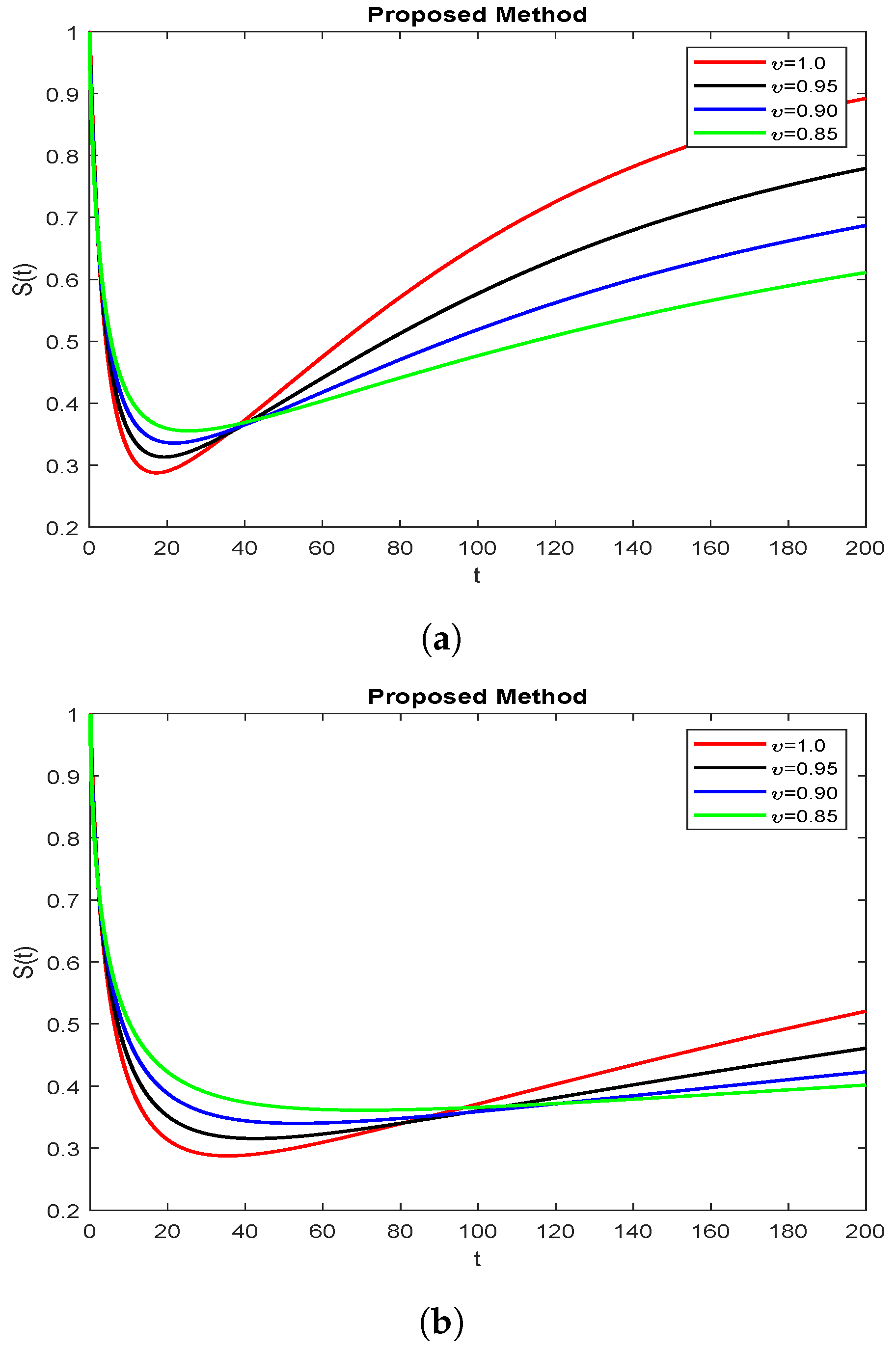
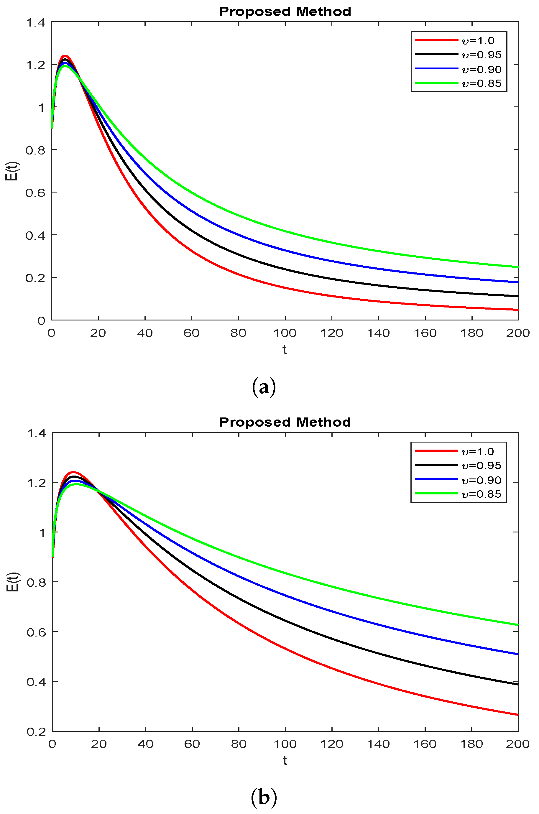
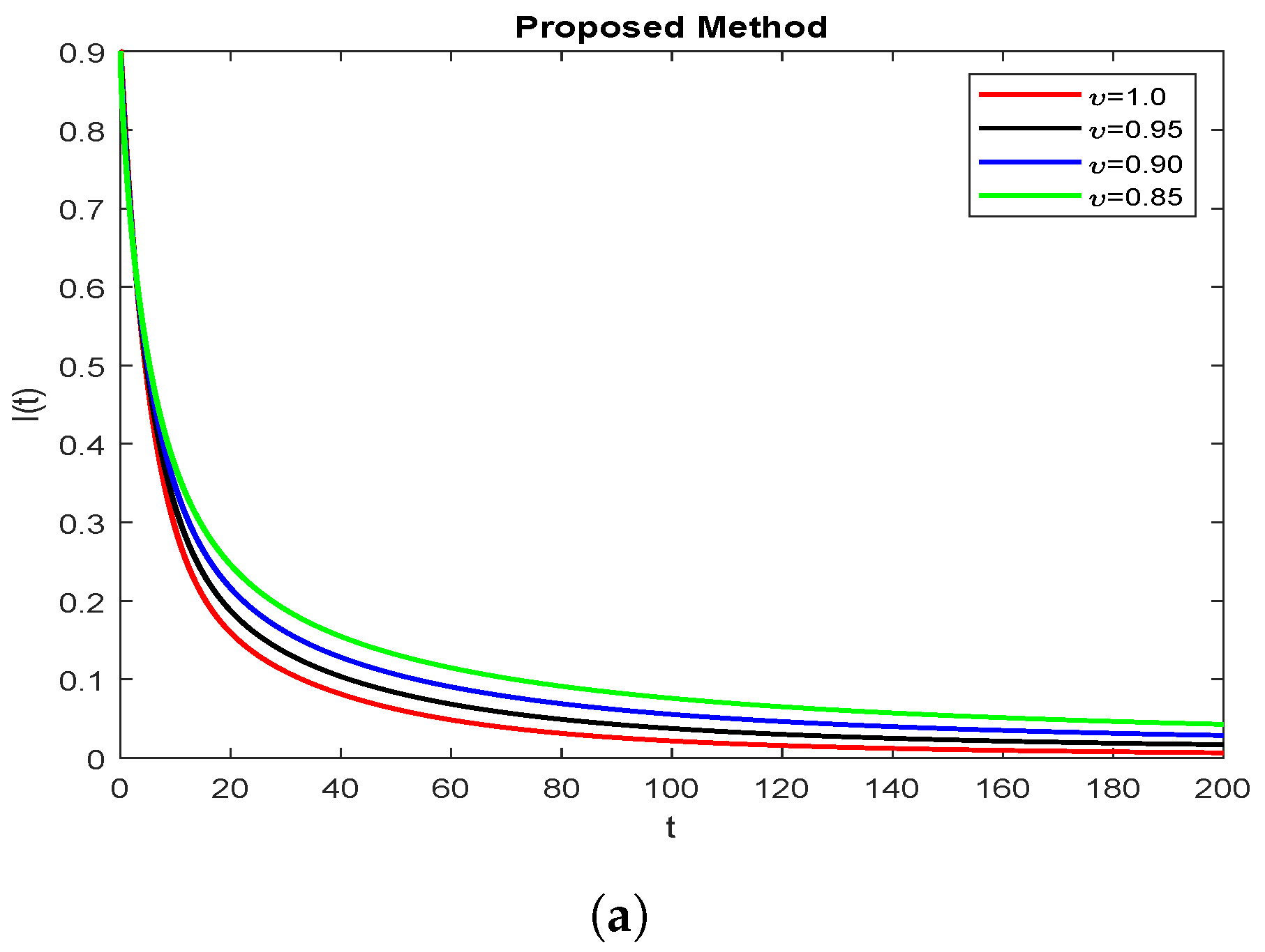
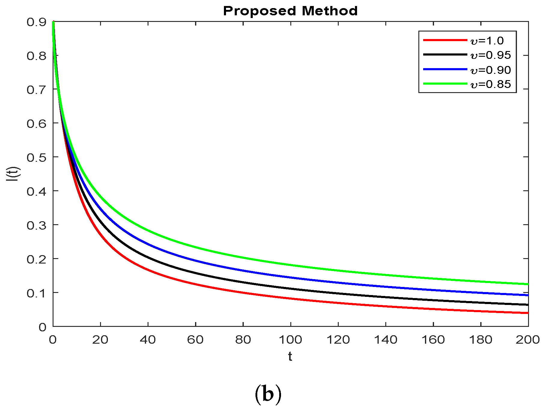
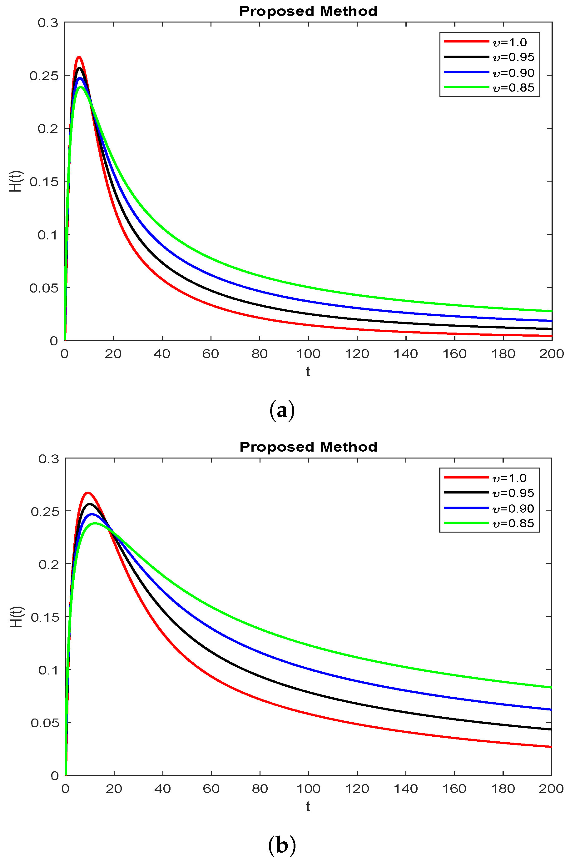
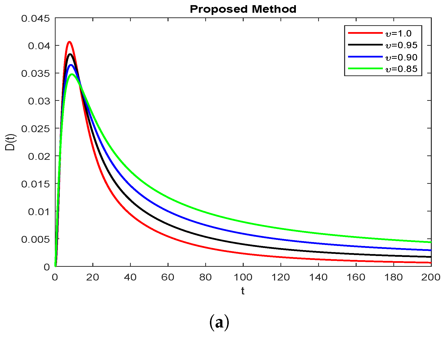
8. Discussions and Numerical Simulations

A mathematical analysis has been performed on a non-linear epidemiological model of the Ebola virus and therapy. In order to ascertain the benefits of the parameters used in this Ebola dynamics model, several simulation tests based on parameter values were carried out to assess the impact of the fractional derivative on the treatment sections. Through using a fractal fractional derivative, the model creates numerical representations for a range of fractional values in accordance with the steady state point. Many numerical methods may be used to study the end time value of a certain parameter in order to analyze how distinct parameters affect the dynamics of the fractional order model. Figure 1, Figure 2, Figure 3, Figure 4, Figure 5 and Figure 6 show graphs of the approximations of solutions for various fractional orders. As shown in Figure 1, Figure 2, Figure 3, Figure 4, Figure 5 and Figure 6, $S\left(t\right)$ and $R\left(t\right)$ increase as the fractional values drop, whereas $E\left(t\right)$, $I\left(t\right)$, $H\left(t\right)$ and $D\left(t\right)$ fall as the fractional values grow. When the fractional values are reduced, the behaviour in all graphs shifts, suggesting that the roots will work better if the fractional values are lower than the classical derivative. These simulations demonstrate how variations in values have an effect on the model behavior. The simulation also demonstrates how the condition of Ebola patients might change over time. As a result, the research becomes even more crucial for making choices and putting restrictions in place.

Through using different numerical techniques and the time fractional parameters, the mechanical characteristics of the fractional order model have been identified. Simulations reveal that the model’s dynamics have changed. Furthermore, with aid of the fractional value and results from various dimensions, the outcomes of the nonlinear system memory were also discovered. It provides a better way to control the disease without defining other parameters. Figure 1 shows the simulations obtained by the power law kernel method. It is highlighted that, when compared to the classical order situation with varied dimensions, the most visible and robust part (the fractional order derivatives) are far better at explaining the physical processes. The numerical results demonstrate how the dynamics in the different fractional orders behave.

Figure 1. Simulation of the model classes with the Caputo fractional derivative. (a) $S\left(t\right)$ at dimension 1. (b) $S\left(t\right)$ at dimension 0.8.

Simulations obtained by the power law kernel approach are shown in Figure 2. It is highlighted that, when compared to the classical order situation with varied dimensions, the most visible and robust parts (the fractional order derivatives) are far better at explaining the physical processes. The numerical results demonstrate how the dynamics in the different fractional orders behave.

Figure 2. Simulation of model classes with the Caputo fractional derivative. (a) $E\left(t\right)$ at dimension 1. (b) $E\left(t\right)$ at dimension 0.8.

Simulations obtained by the power law kernel approach are shown in Figure 3. It is highlighted that, when compared to the classical order situation with varied dimensions, the most visible and robust part (the fractional order derivatives) are far better at explaining the physical processes. The numerical results demonstrate how the dynamics in the different fractional orders behave.

Figure 3. Simulation of model classes with the Caputo fractional derivative. (a) $I\left(t\right)$ at dimension 1. (b) $I\left(t\right)$ at dimension 0.8.

Simulations obtained by the power law kernel approach are shown in Figure 4. It is highlighted that, when compared to the classical order situation with varied dimensions, the most visible and robust parts (the fractional order derivatives) are far better at explaining the physical processes. The numerical results demonstrate how the dynamics in the different fractional orders behave.

Figure 4. Simulation of model classes with the Caputo fractional derivative. (a) $H\left(t\right)$ at dimension 1. (b) $H\left(t\right)$ at dimension 0.8.

Simulations obtained by the power law kernel approach are shown in Figure 5. It is highlighted that, when compared to the classical order situation with varied dimensions, the most visible and robust parts (the fractional order derivatives) are far better at explaining the physical processes. The numerical results demonstrate how the dynamics in the different fractional orders behave.

Figure 5. Simulation of model classes with the Caputo fractional derivative. (a) $R\left(t\right)$ at dimension 1. (b) $R\left(t\right)$ at dimension 0.8.

Simulations obtained by the power law kernel approach are shown in Figure 6. It is highlighted that, when compared to the classical order situation with varied dimensions, the most visible and robust parts (the fractional order derivatives) are far better at explaining the physical processes. The numerical results demonstrate how the dynamics in the different fractional orders behave.

Figure 6. Simulation of model classes with the Caputo fractional derivative. (a) $D\left(t\right)$ at dimension 1. (b) $D\left(t\right)$ at dimension 0.8.

9. Conclusions

To better comprehend how the Ebola virus spreads, a nonlinear compartmental model has been suggested. Six components make up the suggested paradigm, and they are all mutually exclusive. It has been determined that there have been many Ebola virus fever cases and Ebola has caused many fatalities and it may be spread by treating infected individuals and through dead bodies. We were able to analyze the consequences of the Ebola virus on individuals, as well as the general population in any nation, through the research of a proposed mathematical model with fast and slow observable cases. The model’s nonlinear ordinary differential equations were carefully analyzed for the degree to which they are well posed. The existence and positivity of solutions were also checked to determine biological feasibility of the model. Then, we investigated the stability of the iterative scheme of the proposed model by using fixed point theory results. The numerical results were discussed through graphs, and we also compared the results in two different dimensions for a complex analysis. Symmetry analysis is a strong tool that makes it possible to generate numerical answers to given fractional differential equations very methodically. This unique method of fusing two operators was used to derive numerical outcomes and simulations for this purpose. The method is extremely dependable, efficient and capable of resolving a variety of technical and scientific issues. This area of research is beneficial for understanding how the Ebola virus spreads and how to manage illnesses in a community.

References

1. Baseler, L.; Chertow, D.S.; Johnson, K.M.; Feldmann, H.; Morens, D.M. The pathogenesis of Ebola virus disease. Ann. Rev. Pathol. 2017, 12, 387–418. [Google Scholar] [CrossRef]
2. Sullivan, N.J.; Sanchez, A.; Rollin, P.E.; Yang, Z.Y.; Nabel, G.J. Development of a preventive vaccine for Ebola virus infection in primates. Nature 2000, 408, 605–609. [Google Scholar] [CrossRef]
3. Rachah, A.; Torres, D.F. Mathematical modelling, simulation, and optimal control of the 2014 Ebola outbreak in West Africa. Discr. Dyn. Nat. Soc. 2015. [Google Scholar] [CrossRef]
4. Area, I.; Batarfi, H.; Losada, J.; Nieto, J.J.; Shammakh, W.; Torres, A. On a fractional order Ebola epidemic model. Adv. Diff. Equ. 2015, 2015, 278. [Google Scholar] [CrossRef]
5. Rachah, A.; Torres, D.F. Predicting and controlling the Ebola infection. Math. Methods Appl. Sci. 2017, 40, 6155–6164. [Google Scholar] [CrossRef]
6. Kilbas, A.A.; Srivastava, H.M.; Trujillo, J.J. Theory and Applications of Fractional Differential Equations; Elsevier: Amsterdam, The Netherlands, 2006; Volume 204. [Google Scholar]
7. Sun, H.; Zhang, Y.; Baleanu, D.; Chen, W.; Chen, Y. A new collection of real world applications of fractional calculus in science and engineering. Commun. Nonlinear Sci. Numer. Simul. 2018, 64, 213–231. [Google Scholar] [CrossRef]
8. Akg, A. A novel method for a fractional derivative with non-local and non-singular kernel. Chaos. Solitons Fractals 2018, 114, 478–482. [Google Scholar]
9. Akg, E.K. Solutions of the linear and nonlinear differential equations within the generalized fractional derivatives. Chaos Interdiscip. J. Nonlinear Sci. 2019, 29, 023108. [Google Scholar]
10. Diethelm, K.; Ford, N.J. Multi-order fractional differential equations and their numerical solution. Appl. Math. Comput. 2004, 154, 621–640. [Google Scholar] [CrossRef]
11. Fernandez, A.; Baleanu, D.; Fokas, A.S. Solving PDEs of fractional order using the unified transform method. Appl. Math. Comput. 2018, 339, 738–749. [Google Scholar] [CrossRef]
12. Atangana, A.; Baleanu, D. New fractional derivatives with nonlocal and non-singular kernel: Theory and application to heat transfer model. arXiv 2016, arXiv:1602.03408. [Google Scholar] [CrossRef]
13. Atangana, A.; Goufo, E.F.D. On the mathematical analysis of Ebola hemorrhagic fever: Deathly infection disease in west african countries. BioMed Res. Int. 2014, 1–8. [Google Scholar] [CrossRef] [PubMed]
14. Koca, I. Modelling the spread of ebola virus with Atangana-Baleanu fractional operators. Eur. Phys. J. Plus 2018, 133, 100. [Google Scholar] [CrossRef]
15. Latha, V.P.; Rihan, F.A.; Rakkiyappan, R.; Velmurugan, G. A fractional-order model for Ebola virus infection with delayed immune response on heterogeneous complex networks. J. Comput. Appl. Math. 2018, 339, 134–146. [Google Scholar] [CrossRef]
16. Singh, H. A new numerical algorithm for fractional model of Bloch equation in nuclear magnetic resonance. Alexandria Eng. J. 2016, 55, 2863–2869. [Google Scholar] [CrossRef]
17. Singh, H. Operational matrix approach for approximate solution of fractional model of Bloch equation. J. King Saud Univ.-Sci. 2017, 29, 235–240. [Google Scholar] [CrossRef]
18. Dokuyucu, M.A.; Celik, E.; Bulut, H.; Baskonus, H.M. Cancer treatment model with the Caputo-Fabrizio fractional derivative. Eur. Phys. J. Plus 2018, 133, 92. [Google Scholar] [CrossRef]
19. Xu, C.; Farman, M.; Hasan, A.; Akgl, A.; Zakarya, M.; Albalawi, W.; Park, C. Lyapunov Stability and Wave Analysis of COVID-19 Omicron Variant of Real Data with Fractional Operator. Alex. Eng. J. 2022, 61, 11787–11802. [Google Scholar] [CrossRef]
20. Farman, M.; Akg, A.; Abdeljawad, T.; Naik, P.A.; Bukhari, N.; Ahmad, A. Modeling and analysis of fractional order Ebola virus model with Mittag–Leffler kernel. Alex. Eng. J. 2022, 61, 2062–2073. [Google Scholar] [CrossRef]
21. Farman, M.; Akg, l.A.; Nisar, K.S.; Ahmad, D.; Ahmad, A.; Kamangar, S.; Saleel, C.A. Epidemiological analysis of fractional order COVID-19 model with Mittag–Leffler kernel. AIMS Math. 2022, 7, 756–783. [Google Scholar] [CrossRef]
22. Farman, M.; Akg, A.; Tekin, M.T.; Akram, M.M.; Ahmad, A.; Mahmoud, E.E.; Yahia, I.S. Fractal fractional-order derivative for HIV/AIDS model with Mittag–Leffler kernel. Alex. Eng. J. 2022, 61, 10965–10980. [Google Scholar] [CrossRef]
23. Farman, M.; Saleem, M.U.; Ahmad, A.; Ahmad, M.O. Analysis and numerical solution of SEIR epidemic model of measles with non-integer time fractional derivatives by using Laplace Adomian Decomposition Method. Ain Shams Eng. J. 2018, 9, 3391–3397. [Google Scholar] [CrossRef]
24. Amin, M.; Farman, M.; Akg, A.; Partohaghighi, M.; Jarad, F. Computational analysis of COVID-19 model outbreak with singular and nonlocal operator. AIMS Math. 2022, 7, 16741–16759. [Google Scholar] [CrossRef]
25. Seck, R.; Ngom, D.; Ivorra, B.; Ramos, M. An optimal control model to design strategies for reducing the spread of the Ebola virus disease. Math. Biosci. Eng. 2022, 19, 1746–1774. [Google Scholar] [CrossRef]
26. Veeresha, P.; Prakasha, D.G.; Baskonus, H.M. New numerical surfaces to the mathematical model of cancer chemotherapy effect in Caputo fractional derivatives. Chaos Interdiscip. J. Nonlinear Sci. 2019, 29, 013119. [Google Scholar] [CrossRef]