Offline Computation of the Explicit Robust Model Predictive Control Law Based on Deep Neural Networks

Abstract

A significant challenge in robust model predictive control (MPC) is the online computational complexity. This paper proposes a learning-based approach to accelerate online calculations by combining recent advances in deep learning with robust MPC. The use of soft constraint variables addresses feasibility issues in the robust MPC design, while the employment of a symmetrical structure deep neural network (DNN) approximates the robust MPC control law. The symmetry of the network structure facilitates the training process. The use of soft constraints expands the feasible region and also increases the complexity of the training data, making the network difficult to train. To overcome this issue, a dataset construction method is employed. The performance of the proposed method is demonstrated through simulated examples, and the proposed algorithm can be applied to control systems in various fields such as aerospace, three-dimensional printing, optical imaging, and chemical production.

1. Introduction

Robust model predictive control (MPC) synthesis is a popular technique for the control of dynamical systems which solves online dynamic optimization problems, ensuring the stability of the overall closed-loop system with uncertainties [1,2,3,4]. The technique involves an enormous computation time due to the online solution of an optimization problem. Therefore, explicit robust MPC with a short deterministic running time was proposed in [5,6,7,8,9]. For linear systems, the explicit control law can be calculated offline by solving a multi-parameter quadratic programming problem, which eliminates the online optimization process. For a broad class of systems, the nominal performance cost was introduced to calculate the explicit control law in [10,11,12,13,14]. A robust model predictive controller can be designed based on the explicit control law [15,16,17].

Recently, there has been increasing interest in using deep learning-based methods to design model predictive controllers, particularly in industrial and real-world applications [18,19,20,21,22,23]. Among the deep learning models, deep neural networks (DNNs) have been used as controllers in plant models [24]. Due to their structure with multilayer feedforward networks, DNNs have a strong ability to approximate a system’s dynamics. In addition, the deep neural network’s parallelized architecture enables it to be accelerated by the use of a GPU, resulting in real-time response speeds. A DNN-based controller with guaranteed robustness was proposed in [25,26,27,28]. However, most of the related work focuses on the use of DNNs in robust MPC problems with hard constraints. Enforcing hard constraints in robust MPC can lead to conservative results or even infeasibility, resulting in failure of the robust MPC design.

Moreover, the predictive accuracy of the DNN directly impacts the stability and constraint satisfaction of the DNN controller, as highlighted in [25,29,30]. Proposals for DNN controllers with exceptional predictive accuracy can be found in [7]. In the DNN model, the dataset is generated from the domain of attraction, and the distribution of the dataset has a direct effect on the predictive accuracy. However, the constraints of robust MPC dictate the distribution of the state. The training process becomes challenging for datasets with high variability [31], particularly when attempting to achieve a higher predictive accuracy for out-of-distribution data [32]. On the other hand, larger network sizes are often required to achieve a high predictive accuracy without overfitting. The DNN controller is implemented through the feedforward propagation of the neural network [33,34], and large-scale networks increase the computation delay in feedforward propagation.

To tackle the aforementioned challenges, a DNN controller with a symmetrical structure is proposed in this paper. The primary focus is on linear systems, and the DNN is employed to represent the explicit robust MPC. Feasibility of the robust MPC is guaranteed through the use of slack variables to soften the constraints, thereby extending the domain of attraction [35]. Additionally, the robust stability of the DNN controller is ensured by imposing a bound on the permissible input disturbance, as previously proposed in [25,36]. Symmetrical neural networks have demonstrated improved performance in certain scenarios [37,38]. In this study, the primary objective of utilizing a symmetrical network structure is to decrease the size of the network, mitigate the risk of overfitting caused by training, and minimize the maximum allowable computation delay for the DNN controller. The proposed method addresses the feasibility problem through the use of soft constraints and calculates the domain of attraction accordingly. The DNN controller is then obtained by learning the domain of attraction. During the learning process, an admissible control input disturbance is incorporated as a constraint in the network training. The predictive stability of the DNN controller is evaluated by utilizing the empirical risk method to ensure its robustness.

The main contributions of the paper are threefold. First, we propose a DNN-based predictive controller that is designed through an online robust MPC approach with soft constraints in the linear matrix inequality (LMI) framework. Secondly, we introduce the data density-based segmentation method (DDSD) for construction of the dataset, making the network training process more robust. Thirdly, a symmetrical DNN is utilized to approximate the implicit control law, which enhances the online computation performance and reduces the potential risk of overfitting.

2. Problem Description

Consider a discrete time-varying uncertain plant with the following state space equations:

$$x(k+1)=A\left(k\right)x\left(k\right)+B\left(k\right)u\left(k\right),k\ge 0,$$

(1)

where the control move and the state are denoted by $u\left(k\right)\in {\mathbb{R}}^m$ and $x\left(k\right)\in {\mathbb{R}}^n$, respectively, and k is the sampling time. The following constraints are considered:

$$\begin{array}{ccc}\hfill -\overline{u}& \le u(k+i)\le \overline{u},\hfill & \hfill \forall i\ge 0,\end{array}$$

(2a)

$$\begin{array}{ccc}\hfill -\overline{\psi }& \le \mathsf{\Psi }x(k+i+1)\le \overline{\psi },\hfill & \hfill \forall i\ge 0,\end{array}$$

(2b)

where $\overline{u}:={[{\overline{u}}_1,{\overline{u}}_2,\cdots ,{\overline{u}}_m]}^T$, $\overline{\psi }:={[{\overline{\psi }}_1,{\overline{\psi }}_2,\cdots ,{\overline{\psi }}_q]}^T$, and $\mathsf{\Psi }\in {\mathbb{R}}^{q\times n}$.

Suppose that $\left[A\right(k\left)B\right(k\left)\right]\in \Omega$, $\forall k\ge 0$. For polytopic systems, the polytope $\Omega =\mathrm{Co}\{\left[A_1{B}_1\right],\left[A_2{B}_2\right],\cdots ,\left[A_G{B}_G\right]\}$; in other words,

there are G non-negative parameters denoted by ${\omega }_g\left(k\right)$ such that

$$\sum _{g=1}^G{\omega }_g\left(k\right)=1,\left[A\left(k\right)B\left(k\right)\right]=\sum _{g=1}^G{\omega }_g\left(k\right)\left[A_g{B}_g\right].$$

(3)

where $G=1$ corresponds to the nominal linear time-invariant (LTI) system. Without loss of the generality, we follow the pioneer work on robust MPC design (e.g., the work presented in [1]) to establish the problem to solve. Consider that the nominal model that approximates the actual plant is denoted by $[\widehat{A},\widehat{B}]\in \Omega$ (e.g., as $[\widehat{A},\widehat{B}]={\sum }_{g=1}^G\left[A_g{B}_g\right]/G$) [5]. Now, a robust MPC structure should be appropriately constructed to tend the states of the systems in Equations (1), (2a) and (2b) to the equilibrium point $(x_{ss},u_{ss})=(0,0)$. This could be achieved by minimizing the performance index $J_{true,\infty }={\sum }_{i=0}^{\infty }\left[{\parallel x\left(i\right)\parallel }_{{\mathcal{Q}}_1}^2+{\parallel u\left(i\right)\parallel }_{\mathcal{R}}^2\right]$, where ${\mathcal{Q}}_1$ and $\mathcal{R}$ are positive weights. Due to model uncertainty, $J_{true,\infty }$ could not be optimized directly. According to [1], the following optimization problem should be solved for each sampling time k:

$$\begin{array}{cc}\hfill & \underset{u(k+i|k)=F(k\left)x\right(k+i\left|k\right),P\left(k\right)}{min}\underset{\left[A\right(k+i\left)\right|B(k+i)]\in \Omega ,i\ge 0}{max}{J}_{\infty }\left(k\right)\hfill \end{array}$$

$$\begin{array}{cc}\hfill & =\sum _{i=0}^{\infty }\left[{∥x\left(k+i|k\right)∥}_{{\mathcal{Q}}_1}^2+{∥u\left(k+i|k\right)∥}_{\mathcal{R}}^2\right],\hfill \\ \hfill & \mathrm{s}.\mathrm{t}.\left(2\right)\mathrm{and}\hfill \\ \hfill & x(k+i+1|k)=A(k+i\left)x\right(k+i\left|k\right)\hfill \end{array}$$

(4a)

$$\begin{array}{cc}\hfill & +B(k+i)u(k+i|k),x(k\left|k\right)=x\left(k\right),\forall i\ge 0,\hfill \\ \hfill & {∥x\left(k+i+1|k\right)∥}_{P\left(k\right)}^2-{∥x\left(k+i|k\right)∥}_{P\left(k\right)}^2\hfill \\ \hfill & \le -{∥x\left(k+i|k\right)∥}_{{\mathcal{Q}}_1}^2-{∥u\left(k+i|k\right)∥}_{\mathcal{R}}^2,P\left(k\right)>0,\hfill \end{array}$$

(4b)

$$\begin{array}{cc}\hfill & \forall \left[A\right(k+i\left)\right|B(k+i)]\in \Omega ,\forall i\ge 0.\hfill \end{array}$$

(4c)

where $F\left(k\right)$ is the state feedback control law, $x(k+i|k)$ is the predicted state at time $k+i$, based on the measurements at time k. $u(k+i|k),i=0,1,\dots ,m-1$ are m control moves computed by the optimization problem at time k, where m is the control horizon, $u\left(k\right|k)=u(k)$ and $y\left(k\right|k)=y(k)$ are the control move and output to be impemented at time k, respectively, and $y(k+i|k),i=0,1,\dots ,p$ refer to the output measured at time k, where p is the prediction horizon. Moreover, the monotonicity of the cost and robust stability could be realized through Equation (4c). Consider that the closed-loop system is stable. Now, by summing Equation (4c) from $i=0$ to $i=\infty$, we have

$$\underset{\left[A\right(k+i\left)\right|B(k+i)]\in \Omega ,i\ge 0}{max}{J}_{\infty }\left(k\right)\le {∥x\left(k\right)∥}_{P\left(k\right)}^2\le \gamma ,$$

(5)

where $\gamma >0$ represents the robust performance objective function. By substituting $u(k+i|k)=Fx(k+i\left|k\right)$ into Equation (4a–c), we can obtain the inequality

$$\begin{array}{c}x{(k+i\mid k)}^T\left({(A(k+i)+B(k+i)F)}^{T}P(A(k+i)+B(k+i)F)-P\right.\\ \left.+F^{T}RF+Q_1\right)x(k+i\mid k)\le 0.\end{array}$$

This is satified for all $i\ge 0$ if

$${(A(k+i)+B(k+i)F)}^{T}P(A(k+i)+B(k+i)F)-P+F^{T}RF+Q_1\le 0.$$

(6)

By substituting $P=\gamma Q^{-1},Q>0$, substituting $Y=FQ$, and using the Schur complement lemma, then Equation (4c) is equivalent to

$$\left[\begin{array}{cccc}Q& *& *& *\\ A_{g}Q+B_{g}Y& Q& *& *\\ {\mathcal{Q}}^{\frac{1}{2}}Q& 0& \gamma I& *\\ {\mathcal{R}}^{\frac{1}{2}}Y& 0& 0& \gamma I\end{array}\right]\ge 0,g\in \{1,\cdots ,G\},$$

(7)

where $\left[A_g{B}_g\right]$ denotes the vertex of the polytope $\Omega$. The inequality in Equation (7) is affine in $\left[A\right(k+i\left)B\right(k+i\left)\right]$. Hence, it is satisfied for all

$$\left[A(k+i)B(k+i)\right]\in \Omega =\mathrm{Co}\{\left[A_1{B}_1\right],\left[A_2{B}_2\right],\cdots ,\left[A_G{B}_G\right]\}$$

if and only if there exist $Q>0,Y=FQ$ and $\gamma$ such that Equation (7) holds. The feedback matrix is then given by $F=Y{Q}^{-1}$. For the control state $x\left(k\right)$, we have

$$\begin{array}{ccc}\hfill \left[\begin{array}{cc}1& *\\ x\left(k\right)& Q\end{array}\right]& \ge 0,\hfill & \hfill Q>0.\end{array}$$

(8)

Consider that Equations (7) and (8) are fulfilled. Now, to ensure Equation (2a,b), the following inequalities should be realized:

$$\begin{array}{cc}\hfill & \left[\begin{array}{cc}Q& *\\ Y& Z\end{array}\right]\ge 0,Z_{jj}\le {\overline{u}}_j^2,j\in \{1,\cdots ,m\},\hfill \\ \hfill & \left[\begin{array}{cc}Q& *\\ \mathsf{\Psi }(A_{g}Q+B_{g}Y)& \Gamma \end{array}\right]\ge 0,{\Gamma }_{ss}\le {\overline{\psi }}_s^2,s\in \{1,\cdots ,q\},\hfill \end{array}$$

(9)

$$\begin{array}{cc}\hfill & g\in \{1,\cdots ,G\},\hfill \end{array}$$

(10)

where the j-th (s-th) diagonal element of Z ($\Gamma$) is denoted by $Z_{jj}$ (${\Gamma }_{ss}$) and ${\overline{u}}_j>0,{\overline{\psi }}_s>0$. To solve Equation (4a–c), the following constrained optimization problem should be solved:

$$\underset{\gamma ,Q,Y,Z,\Gamma }{min}\gamma ,\mathrm{s}.\mathrm{t}.\left(7\right)–\left(10\right).$$

(11)

To avoid the online solution of optimization problems, offline robust MPC methods were introduced in [5]. Equation (11) can be transformed into the implicit control law in offline methods. In this work, a DNN was utilized to approximate the robust MPC law by representing the implicit control law.

3. Robust Design of a Probability-Based DNN Controller

The goal of the offline robust MPC is to design the state feedback control law. The overall framework is shown in Figure 1.

In the proposed method, the DNN is used to learn the mapping relationship of the gain matrix $F\in {\mathbb{R}}^{m\times n}$ for the state feedback control law:

$$u\left(k\right)=F\left(x\right(k\left)\right),$$

(12)

where $F(·)$ represents the explicit control law. The constructed DNN is used as a DNN controller whose control and predictions horizon are consistent with the learned robust MPC. In order to deal with feasibility issues in the robust MPC, we introduce soft constraints to extended the domain of attraction, which is discussed completely in [35]. For a linear system with uncertainty, soft constraints are designed via linear matrix inequalities (LMIs). The slack variables are added to the LMI, and Equations (9)–(11) are modified as follows:

$$\begin{array}{cc}\hfill & \left[\begin{array}{cc}Q& *\\ Y& Z\end{array}\right]\ge 0,Z_{jj}\le {\beta }_j{\overline{u}}_j^2,j\in \{1,\cdots ,m\},\hfill \\ \hfill & \left[\begin{array}{cc}Q& *\\ \mathsf{\Psi }(A_{g}Q+B_{g}Y)& \Gamma \end{array}\right]\ge 0,{\Gamma }_{ss}\le {\beta }_s{\overline{\psi }}_s^2,\hfill \end{array}$$

(13)

$$\begin{array}{cc}\hfill & s\in \{1,\cdots ,q\},g\in \{1,\cdots ,G\},\hfill \end{array}$$

(14)

where the j-th (s-th) diagonal element of Z ($\Gamma$) is represented by $Z_{jj}$ (${\Gamma }_{ss}$) and ${\beta }_j$ and ${\beta }_s$ are correction factors. Therefore, Equation (4a–c) could be solved by

$$\underset{{\gamma }^{*},Q,Y,Z,\Gamma }{min}{\gamma }^{*},\mathrm{s}.\mathrm{t}.\left(7\right),\left(8\right),\left(13\right),\left(14\right),$$

(15)

where ${\gamma }^{*}={\sum }_{ii=1}^K{\beta }_{ii}$, $K=m+q$. By imposing soft constraints, we obtain a new optimization problem and a state feedback control law that is used as the objective function of the DNN controller. Furthermore, the domain of attraction is extended compared with the original robust MPC. The dataset for training DNNs is constructed from this extended domain of attraction.

3.1. Guaranteeing the Stability of the DNN Controller

In the proposed DNN controller, the network inputs are the states of the system, while the network output represents the control input. To ensure the robustness of the DNN controller, a bound $\eta$ is imposed on the admissible control input disturbance, which is set as the maximum predictive error of the network output. The bound $\eta$ satisfies

$$\eta \le \frac{1}{ϵ}\sqrt{\frac{{\delta }_{\mathrm{loc}}}{c_{\delta ,u}}},$$

(16)

where $ϵ$ is the Lipschitz constant and ${\delta }_{\mathrm{loc}},c_{\delta ,u}\in \mathbb{R}$ are the process parameters. The bound $\eta$ on the admissible control input disturbance in robust MPC is discussed in [28]. In this paper, we only utilize the bound $\eta$ as a constraint in the training of the DNN controller. The DNN controller generates a control input, which ensures that the state $x(k+1)=A\left(k\right)x\left(k\right)+B\left(k\right)u\left(k\right)\in {\mathcal{C}}_{\infty }$ remains within the maximal control invariant set ${\mathcal{C}}_{\infty }$, as detailed in [25]. In the training process, we introduce an indicator function

$$I\left(\mathrm{x}\left(k\right)\right):=\left\{\begin{array}{c}1\mathrm{if}\left|\right|F\left(x\left(k\right)\right)-F_{\mathrm{DNN}}{\left(x\left(k\right)\right)\parallel }_{\infty }\le \eta \hfill \\ 0\mathrm{otherwise}\hfill \end{array}\right.$$

(17)

where $F_{\mathrm{DNN}}\left(x\left(k\right)\right)$ represents a predicted value of the DNN controller. In order to assess the stability of the trained DNN controller, we propose a metric function as follows:

$$\tilde{\mu }:=\frac{1}{p}\sum _{p=1}^{P}I\left(x\left(p\right)\right),$$

(18)

where $x\left(p\right)$ represents a test sample, P represents the number of training samples, and $0<\tilde{\mu }\le 1$. The DNN controller guarantees stability and constraint satisfaction within the domain of attraction if the indicator function $I\left(x\left(p\right)\right)=1,\forall x\left(p\right)$. Therefore, by using this metric as a constraint during the test process, we can ensure the probabilistic robustness of the DNN controller.

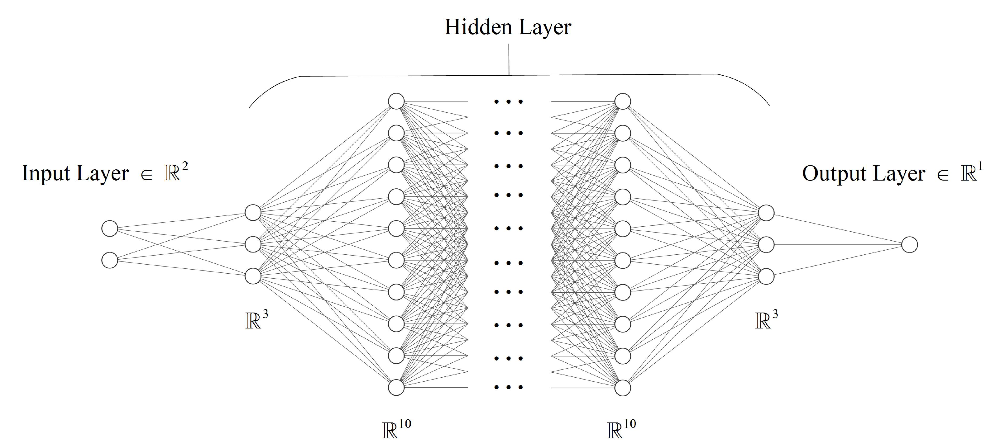
3.2. Network Model and Parameter Updating

The structure of the DNN controller can be represented as follows:

$$\mathcal{N}=\left[n^1,\dots ,n^l,\cdots ,n^L\right],$$

(19)

where $\mathit{N}$ is a vector consisting of network layers, l denotes the index for a network layer, and $n^l$ represents the number of neurons in this layer. The schematic diagram of a DNN is shown in Figure 2.

The quantity of neurons within the input layer, denoted as $n^0$, corresponds to the number of feature inputs. A weight matrix serves as the link between layers, with the weight matrices of the deep neural network represented as a vector:

$$\mathcal{W}=\left[W^1,\dots ,W^l,\dots ,W^L\right],$$

(20)

where $W^l$ is used to connect layers l and $l-1$ and its specific form is as follows:

$$W^l=\left(\begin{array}{ccccc}{w}_{11}^l& \dots & w_{c1}^l& \cdots & w_{n^{l}1}^l\\ ⋮& \ddots & ⋮& \ddots & ⋮\\ w_{1r}^l& \cdots & w_{cr}^l& \cdots & w_{n^{l}r}^l\\ ⋮& \ddots & ⋮& \ddots & ⋮\\ w_{1n^{l-1}}^{\left[l\right]}& \cdots & w_{c{n}^{l-1}}^l& \cdots & w_{n^l{n}^{l-1}}^l\end{array}\right),$$

where $w_{cr}$ is the weight connection between the c-th neuron of layer l and the r-th neuron of layer $l-1$. After applying the affine transformation to the previous layer neurons, the bias of the DNN is obtained:

$$\mathcal{B}=\left[b^1,\dots ,b^l,\dots ,b^L\right],$$

(21)

where $b^l={\left[b_1^l,\dots ,b_c^l,\dots ,b_{n^l}^l\right]}^{\mathrm{T}}$ is the bias of layer l.

The cost function $\mathcal{J}\left(\theta \right)$ is defined as

$$\mathcal{J}\left(\theta \right)=\frac{1}{2}\sum _{p=1}^{m_s}{\left(\widehat{y}{\left(\theta \right)}^{\left(p\right)}-y^{\left(p\right)}\right)}^2,$$

(22)

where p is the index of the samples, $m_s$ is the number of examples in the training set $D_1$, $\widehat{y}{\left(\theta \right)}^{\left(p\right)}$ is the predicted value for the $p^{th}$ sample, and $y^{\left(p\right)}$ is the label for the $p^{th}$ sample. Now, the momentum gradient descent algorithm is employed for updating the DNN parameters. The updated parameters are given as

$$\begin{array}{cc}\hfill & {\mathit{v}}_{d{W}^l}:=\beta {\mathit{v}}_{d{W}^l}+(1-\beta )\frac{\partial \mathcal{J}\left(\theta \right)}{\partial W^l}\hfill \end{array}$$

(23a)

$$\begin{array}{cc}\hfill & {\mathit{v}}_{d{b}^l}:=\beta {\mathit{v}}_{d{b}^l}+(1-\beta )\frac{\partial \mathcal{J}\left(\theta \right)}{\partial b^l}\hfill \end{array}$$

(23b)

$$\begin{array}{cc}\hfill & W^l:=W^l-\alpha {\mathit{v}}_{d{W}^l}\hfill \end{array}$$

(23c)

$$\begin{array}{cc}\hfill & b^l:=b^l-\alpha {\mathit{v}}_{d{b}^l},\hfill \end{array}$$

(23d)

where $\beta$ serves as a hyperparameter that regulates the exponent-weighted average and $\alpha$ denotes the learning rate for adjusting the parameters. The parameters ${\mathit{v}}_{dW}$ and ${\mathit{v}}_{db}$ represent the momentum for $dW$ and $db$, respectively. The weights and biases of every layer in the deep neural network are updated according to Equation (23a–d). To assure the robustness of the DNN controller, Equation (17) is incorporated as a criterion in the training process. Typically, the permissible control input disturbance $\eta$ is scaled by a factor $\gamma$ to account for the discrepancy between network training and testing. In the evaluation process, Equation (18) is utilized to measure the prediction error.

3.3. Training Strategy for the DNN Controller

In the proposed method, the training samples are composed of both system states and control inputs, which are obtained through sampling within the domain of attraction. In principle, as long as the sampling step is sufficiently small, a comprehensive set of system states can be generated from the domain of attraction.

However, regular sampling leads to a dataset that is relatively homogeneous, and partitioning it into training and test sets results in a non-consistent distribution of data across different datasets. Furthermore, shuffling the dataset and then partitioning it disrupts the original data distribution pattern, making it more challenging to train the model for accurate approximation. Specifically, in some cases, taking too small of a sampling step within a fixed range can lead to a lack of diversity within the data, resulting in limited variation between the training and test sets, which increases the risk of overfitting the model during the training process.

To address the issues arising from the construction of the dataset, we propose a data density-based segmentation method (DDSD). By utilizing this method, we can ensure consistent distribution of data samples across different datasets. Taking a two-dimensional attraction domain as an example, we define the data density as the number of samples per unit area. By assuming that the sampling steps are $s_1$ and $s_2$, the data density $\rho$ is given by

$$\rho =\frac{1}{s_1\times s_2}.$$

(24)

We set a benchmark data density of ${\rho }_o={10}^8$ and use this as a reference to define the relative density of the sample set $\mathcal{D}$. The step size for sampling is determined based on the numerical precision of the state quantities, and different states may correspond to different sampling steps.

By varying the sampling step size, we are able to generate datasets with different data densities. To ensure the independence and non-overlapping of the training and test sets, the starting sampling points should be distinct between them. Once the desired data density is obtained, we construct the dataset using samples from the domain of attraction. This dataset comprises three sets: the training set ${\mathcal{D}}_1$, the validation set ${\mathcal{D}}_2$, and the test set ${\mathcal{D}}_3$. The data density of the constructed dataset can be represented as follows:

$${\rho }_{\mathrm{dataset}}=\left[{\rho }_{\mathrm{train}},{\rho }_{\mathrm{valid}},{\rho }_{\mathrm{test}}\right],$$

(25)

where ${\rho }_{\mathrm{train}}$, ${\rho }_{\mathrm{valid}}$, and ${\rho }_{\mathrm{test}}$ are the data densities of the training, validation, and test sets, respectively.

Furthermore, it is sufficient for the chosen data density to align with the numerical precision of the control system state. The dataset generated based on this data density is relatively small in comparison with the total number of possible samples. Utilizing a small number of samples during network training can lead to issues of overfitting. To address this problem, the regularization technique of ridge regression is incorporated into the objective function. In light of this, the cost function of the DNN controller is reformulated as,

$$\mathcal{J}\left(\theta \right)=\frac{1}{2}\sum _{p=1}^{m_s}{\left(\widehat{y}{\left(\theta \right)}^{\left(p\right)}-y^{\left(p\right)}\right)}^2+\frac{\lambda }{2m_s}\sum _{l=1}^L\left|\right|W^l{\left|\right|}^2,$$

(26)

where $\lambda$ represents the penalty factor that determines the degree of penalization applied to the performance index. The process of determining the optimal value of $\lambda$ involves the utilization of the 10 fold cross-validation method. The dataset is first divided into a training set ${\mathcal{D}}_1$ and a test set ${\mathcal{D}}_2$. The training set ${\mathcal{D}}_1$ is then further partitioned 10 validation sets, represented by ${\mathcal{D}}_{1,i}$, where $i\in \{1,\dots ,10\}$. In each iteration of the cross-validation, one validation set is used to evaluate the performance of the model, while the remaining nine sets are used for training. The value of $\lambda$ that corresponds to the highest performance is selected as the optimal value and is subsequently used to compute the final weight matrix:

$$\theta ={\left({a^{L-1}}^T{a}^{L-1}+\lambda I\right)}^{-1}{a^{L-1}}^{T}y,$$

(27)

where $a^{L-1}={\left[a_1^{L-1},\dots ,a_r^{L-1},\cdots ,a_{n^{L-1}}^{L-1}\right]}^T$ is a vector consisting of the activation values for $L-1$ [39].

In the first stage of Algorithm 1, the optimal value $\lambda$ of the regularization parameter is determined through the application of cross-validation experiments. This value is then used to calculate the initial weights for the second stage using Equation (27). In order to achieve a high level of approximation accuracy, as stipulated by Equation (17), it is necessary to minimize the training error. To this end, we employ a data density-based segmentation method (DDSD) to generate multiple sets of test data, which allows for the evaluation of the performance of the DNN controller in both the public and private phases while ensuring that the distribution of data in these sets is independent and homogeneous.

In order to evaluate the performance of the trained DNN controller, a set of test samples are used in the second stage. These test samples, referred to as “public test data”, constitute a dataset that is approximately half the size of the training set. Additionally, in the third stage, the DNN controller’s performance is evaluated using “private test data”, which is not included in the training or public test sets. These private test samples were sampled at different steps from the public test samples, allowing for a more realistic assessment of the performance of the trained model in unseen scenarios.

In addition to the appropriate dataset, the architecture of the neural network is also crucial. In this paper, we utilize a fully connected symmetrical neural network as the architecture of the controller, as it can effectively reduce the network size while preserving its learning capability. To further mitigate the risk of overfitting, techniques such as weight pruning and dropout regularization are also applied to the network.

Algorithm 1 Learn the robust MPC control law using DNN.

1: Generate the domain of abstraction through robust MPC, and construct the dataset consisting of the sample $\left(x\right(k),u(k\left)\right)$ based on Equation (15). 2: Compute the bound $\eta$ based on Equation (16). (Step 1: Ten-fold cross-validation) 3: Initialization: $\theta \leftarrow 0$, ${\lambda }_i=k_i,i=1,2,\dots ,10$, 4: repeat 5:    Update $\theta$ based on Equation (26) 6: until Finish 7: Determine ${\lambda }_i$ and calculate $\theta$ based on Equation (27); (Step 2: Network training based on probabilistic level stability) 8: Initialization: $\theta (W,b)\leftarrow \theta$, 9: repeat 10:    repeat 11:      Update W based on Equation (23c) 12:      Update b based on Equation (23d) 13:      Calculate the metric of the training process based on Equation (18) 14:    until $\frac{1}{p}{\sum }_{p=1}^{P_{train}}I\left(x\left(p\right)\right)\to 1$ 15:    Extract “public test samples” from the test set and evaluate the approximation performance of DNNs based on Equation (18). 16: until$\frac{1}{q}{\sum }_{q=1}^{Q_{test}}I\left(x\left(q\right)\right)>0.9545,Q_{test}$ is the number of “public test samples” 17: Determine $\theta (W,b)$; (Step 3: Testing of network model) 18: Evaluation of network models using “private test samples” from the sample set $\mathcal{D}$; Output:  weight $\theta (W,b)$ of DNN controller.

3.4. Computational Complexity

The computational complexity directly affects the computation delay of the controller. The more computational complexity one has, the more computation resources are required. Under the same conditions, more computation time is required. It is well known that the computational complexity of other explicit RMPC algorithms increases exponentially as the number of system states increases.

The computational complexity of the robust MPC for linear time-varying systems is generally high, as it involves solving a series of quadratic programming (QP) problems at each time step. The complexity of solving a QP problem is typically $O\left(n^3\right)$ for a problem with n decision variables, where n is the dimension of the state space of the system. Additionally, the robust MPC algorithm typically requires the solution of a sequence of these QP problems over a finite horizon, which can further increase the computational complexity. The complexity of the algorithm can be reduced by using efficient numerical methods to solve the QP problems and by approximating the solution to the QP problem.

In this paper, the number of system states is used as a variable to study the computational complexity of the DNN controller. The proposed DNN controller also has less computational complexity than other RMPC offline algorithms. According to Section 3.2, the structure of the DNN controller with the input layer is as follows:

$${\mathcal{N}}_0=\left[n^0,\dots ,n^l,\cdots ,n^L\right].$$

(28)

A feedforward neural network is a composition of layers of computational units which defines a function $f:{\mathbb{R}}^{n^0}\to {\mathbb{R}}^{n^L}$ of the form

$$f_{{\mathcal{N}}_0}(x;\theta )=h^{\mathrm{out}}\circ g^L\circ h^L\circ \cdots \circ g^1\circ h^1\left(x\right),$$

(29)

where x represents $n^0$ and $g^l$ and $h^l$ are a nonlinear activation function and a linear preactivation function in layer l, respectively. The parameter $\theta$ is composed of $W^l\in {\mathbb{R}}^{n^l\times n^{l-1}}$ and bias vectors $b\in {\mathbb{R}}^{n^l}$ for layer l. The input of the l-th layer is a vector $x^l={[x_1^l,\cdots ,x_{n^l}^l]}^T$, which is computed from the activations of the preceding layer by $x^l=g^l\left(h^l\left(x^{l-1}\right)\right)$. Given the activations $x^{l-1}$ of the units in layer $l-1$, the preactivation of layer l is given by

$$h^l\left(x^{l-1}\right)=W^l{x}^{l-1}+b^l$$

(30)

where $h^l={[h_1^l,\cdots ,h_{n^l}^l]}^T$ is an array composed of $n^l$ preactivation values, and $h_i^l$ denotes the value of $h_k^l(·)$. The activation of the i-th unit in layer l is given by

$$x_i^l=g_i^l\left(h_i^l\left(x^{l-1}\right)\right).$$

(31)

According to Equation (29), we define that in the activation of one unit, every multiplication or addition is defined as an operation. In addition, we choose the rectified linear unit function (ReLU) as the activation function and assume that the DNN has a fixed width n. For a DNN with $n^0$ inputs, $n^L$ outputs, and $L-1$ hidden layers of a width $n⩾n^0$, the maximal number of linear regions has a lower bound of

$$\left(\prod _{i=1}^{L-1}{⌊\frac{n^i}{n^0}⌋}^{n^0}\right)\sum _{j=0}^{n^0}\left(\begin{array}{c}{n}^L\\ j\end{array}\right).$$

(32)

Therefore, by utilizing Equation (32), we determine the number of linear regions in the deep neural network implemented with the rectified linear unit (ReLU) activation function, as outlined in [40]. An affine function, comprising both addition and multiplication, serves as a representation of a linear region, resulting in computational complexity that is less than twice the maximum number of linear regions. The architecture of the deep neural network can be designed based on computational speed and memory needs.

4. Experimental Results

In this section, we present an example to illustrate the practical application of the proposed DNN-based method. In the example, the GPU version of PyTorch 1.12 in a Python environment is employed for training and testing the network performance of the DNN, as well as for computing the closed-loop responses. Additionally, the LMI Control Toolbox in a Matlab environment is used to compute the solution to the linear objective minimization problem and the closed-loop responses of the robust MPC. No optimization was carried out to improve the training time, and the software was executed on the AMD 5900X (CPU) and 2080Ti (GPU) hardware platforms.

In this section, we present a numerical example to illustrate the capabilities of the DNN controller. Consider the polytopic system in Equation (33), with $\Omega$ being defined by Equation (34):

$$\begin{array}{c}\hfill x(k+1)=A\left(k\right)x\left(k\right)+B\left(k\right)u\left(k\right)+\omega \times \left[\begin{array}{c}0.00022\hfill \\ 0.00564\hfill \end{array}\right],\\ \hfill y\left(k\right)=\left[01\right]\times x\left(k\right)+0.1,\end{array}$$

(33)

where $\omega$ is a is a random number between 0 and 1 and

$$\begin{array}{cc}\hfill & A_1=\left[\begin{array}{cc}0.8227\hfill & -0.0017\hfill \\ 6.1233\hfill & 0.9367\hfill \end{array}\right],A_2=\left[\begin{array}{cc}0.9654& -0.0018\\ -0.6759& 0.9433\end{array}\right],\hfill \\ \hfill & A_3=\left[\begin{array}{cc}0.8895\hfill & -0.0029\hfill \\ 2.9447\hfill & 0.9968\hfill \end{array}\right],A_4=\left[\begin{array}{cc}0.8930& -0.0006\\ -2.7738& 0.8864\end{array}\right],\hfill \\ \hfill & B_1=\left[\begin{array}{c}-0.0001\\ 0.1014\end{array}\right],B_2=\left[\begin{array}{c}-0.0001\\ 0.1016\end{array}\right],\hfill \\ \hfill & B_3=\left[\begin{array}{c}-0.0002\\ 0.1045\end{array}\right],B_4=\left[\begin{array}{c}-0.000034\\ 0.0986\end{array}\right].\hfill \end{array}$$

(34)

For the system under consideration, the chosen weight matrices for the state and control objectives were $Q_1=9$ and $R=1$, respectively. Additionally, the upper bounds for the state vector and control move were set to 100. By utilizing the above-mentioned model parameters, we could obtain the state feedback control law $F\left(x\right(k\left)\right)$ using the robust MPC method. Given a set of system states $(x_1,x_2)$ within the domain of attraction, the corresponding control input u was computed. The DNN controller used the pairs of $(x_1,x_2,u)$ as training samples. Therefore, by sampling a large number of points within the domain of attraction, we could generate a dataset for training the DNN controller.

As per the design of DDSM, we set the sampling step sizes to 0.001 and 0.01. The data density of the dataset was represented as $[0.0413,0.0041,0.00634].$ Additionally, before training the DNN, we predefined the hyperparameters of the network. The learning rate $\alpha$ was set to 0.0001, and the exponentially weighted average $\beta$ was set to 0.9. The structure of the DNN controller was instantiated as a real row vector [3, 10, 25, 80, 400, 400, 80, 25, 10, 3], which represents a symmetrical DNN. Through cross-validation tests, we calculated a series of penalty factors $\lambda$. The value of $\lambda$ with the minimum value ($\lambda =5$) was used as the regularization term in the DNN.

Furthermore, we calculated the admissible control input disturbance $\eta =7.1\times {10}^{-3}$ according to the robust MPC method. The detailed discussion and proof for $\eta$ can be found in [28]. The optimization algorithm used for training the DNN was set to the mini-batch gradient descent algorithm, and the size of the mini-batch was set to 10.

The trained DNN controller is a good approximation of the state feedback control law. This is demonstrated through the visualization of the DNN controller, presented in Figure 3a. To train the DNN controller, a sample size of 251,001 was utilized, with the control policy of the DNN controller represented on the z-axis. To evaluate the performance of the DNN controller, a sample size of 384 was employed, utilizing a test set that was independent of the data samples used in training. This was achieved by utilizing distinct data densities for sampling during the dataset construction process.

In training the deep neural network controller, a sample size of 251,001 was utilized, with the control policy of the DNN controller represented on the z-axis. A private test set with 384 samples was employed in evaluating the performance of the deep neural network controller by utilizing a test set that was independent of the data samples used in training, which was achieved through the utilization of distinct data densities for sampling.

The deep neural network (DNN) used in this study demonstrated strong learning capabilities, allowing it to effectively capture the global behavior of the state feedback control law. Training was performed using an NVIDIA GXT 2080Ti graphics processing unit, with a single training session taking approximately 8 h. The DNN controller was evaluated using a private test set, with the results of the error analysis presented in

Table 1. Test error of DNN controller.

Error	Control Strategy
	(−60,−40]	(−40,−20]	(−20,0]	[0,20]	(20,40]	(40,60)
Max (${10}^4$)	6.5	6.7	6.8	6.9	6.6	6.5
Mean (${10}^{-5}$)	5.2	5.3	5.5	5.5	5.4	5.2

. Overall, the DNN controller demonstrated low prediction error during testing.

In Table 1, we presented the predictive values, which were divided into six intervals. To evaluate the prediction accuracy of the controller, we used both the maximum error and the average error. As per our training method, the maximum prediction accuracy in each interval was less than the admissible control input disturbance threshold of $\eta =7.1\times {10}^{-3}$. This demonstrates that the DNN is capable of effectively approximating the state feedback control law of robust MPC. As a result, the DNN controller can be effectively utilized in the online control of systems. The phase trajectories for the robust MPC method, the improved offline method, and the DNN controller are illustrated in Figure 4, given the current states.

Figure 5 illustrates the phase trajectories of different initial states and the results over time for a specific initial state. In order to evaluate the online computation time of the DNN controller, we compared it to the online solution of the robust MPC for 200 samples within the domain of attraction. The evaluation of the robust MPC took an average of 0.33 s per point, while the offline and improved offline method took an average of 0.596 and 0.431 ms, respectively. The DNN controller, however, was significantly faster, taking only 0.3 ms on average, which was 1100 times faster than the robust MPC and improved offline methods. Unlike other robust controllers, the response time of the DNN controller is not dependent on the prediction horizon. This highlights the potential for speeding up even further which can be achieved by using the DNN controller.

5. Conclusions

In this paper, we proposed a novel DNN controller for learning state feedback control laws. The approach includes the utilization of soft constraints in the LMI design of robust MPC to address feasibility issues in the design of the controller. During the training of the neural network controller, a bound on the control input disturbance is imposed as a constraint on the prediction error. Additionally, cross-validation experiments were implemented to increase the universality of the test set, thereby enhancing the generalization of the DNN controller within the domain of attraction. To mitigate the potential risk of overfitting, a dataset construction method was proposed. Future work includes the exploration of alternative learning algorithms and more general verification using different indicator functions for applications in higher-dimensional systems.

References

1. Kothare, M.V.; Balakrishnan, V.; Morari, M. Robust constrained model predictive control using linear matrix inequalities. Automatica 1996, 32, 1361–1379. [Google Scholar] [CrossRef] [Green Version]
2. Kouvaritakis, B.; Rossiter, J.A.; Schuurmans, J. Efficient robust predictive control. IEEE Trans. Autom. Control 2000, 45, 1545–1549. [Google Scholar] [CrossRef]
3. Angeli, D.; Casavola, A.; Mosca, E. Ellipsoidal low-demanding MPC schemes for uncertain polytopic discrete-time systems. In Proceedings of the 41st IEEE Conference on Decision and Control, Vols 1–4, Las Vegas, NV, USA, 10–13 December 2002; pp. 2935–2940. [Google Scholar]
4. Wan, Z.Y.; Kothare, M.V. Efficient robust constrained model predictive control with a time varying terminal constraint set. Syst. Control. Lett. 2003, 48, 375–383. [Google Scholar] [CrossRef]
5. Wan, Z.Y.; Kothare, M.V. An efficient off-line formulation of robust model predictive control using linear matrix inequalities. Automatica 2003, 39, 837–846. [Google Scholar] [CrossRef]
6. Sui, D.; Feng, L.; Ong, C.J.; Hovd, M. Robust explicit model predictive control for linear systems via interpolation techniques. Int. J. Robust Nonlinear Control 2010, 20, 1166–1175. [Google Scholar] [CrossRef]
7. Tian, X.; Peng, H.; Zhou, F.; Peng, X. A synthesis approach of fast robust MPC with RBF-ARX model to nonlinear system with uncertain steady status information. Appl. Intell. 2021, 51, 19–36. [Google Scholar] [CrossRef]
8. Hu, Z.; Shi, P.; Wu, L. Polytopic Event-Triggered Robust Model Predictive Control for Constrained Linear Systems. IEEE Trans. Circuits Syst. Regul. Pap. 2021, 68, 2594–2603. [Google Scholar] [CrossRef]
9. Zamani, A.; Bolandi, H. Continuous-time Nonlinear Robust MPC for Offset-free Tracking of Piece-wise Constant Setpoints with Unknown Disturbance. Int. J. Control Autom. Syst. 2022, 20, 1063–1075. [Google Scholar] [CrossRef]
10. Ding, B.C.; Xi, Y.G.; Cychowski, M.T.; O’Mahony, T. Improving off-line approach to robust MPC based-on nominal performance cost. Automatica 2007, 43, 158–163. [Google Scholar] [CrossRef]
11. Dai, L.; Yu, Y.; Zhai, D.H.; Huang, T.; Xia, Y. Robust model predictive tracking control for robot manipulators with disturbances. IEEE Trans. Ind. Electron. 2020, 68, 4288–4297. [Google Scholar] [CrossRef]
12. Preitl, Z.; Precup, R.E.; Tar, J.K.; Takács, M. Use of multi-parametric quadratic programming in fuzzy control systems. Acta Polytech. Hung. 2006, 3, 29–43. [Google Scholar]
13. Precup, R.E.; David, R.C.; Roman, R.C.; Petriu, E.M.; Szedlak-Stinean, A.I. Slime mould algorithm-based tuning of cost-effective fuzzy controllers for servo systems. Int. J. Comput. Intell. Syst. 2021, 14, 1042–1052. [Google Scholar] [CrossRef]
14. Ucgun, H.; Okten, I.; Yuzgec, U.; Kesler, M. Test Platform and Graphical User Interface Design for Vertical Take-Off and Landing Drones. Sci. Technol. (ROMJIST) 2022, 25, 350–367. [Google Scholar]
15. Bumroongsri, P.; Kheawhom, S. An off-line robust MPC algorithm for uncertain polytopic discrete-time systems using polyhedral invariant sets. J. Process Control 2012, 22, 975–983. [Google Scholar] [CrossRef]
16. Tang, X.; Qu, H.; Wang, P.; Zhao, M. Constrained off-line synthesis approach of model predictive control for networked control systems with network-induced delays. ISA Trans. 2015, 55, 135–144. [Google Scholar] [CrossRef]
17. Zhang, K.; Shi, Y. Adaptive model predictive control for a class of constrained linear systems with parametric uncertainties. Automatica 2020, 117, 108974. [Google Scholar] [CrossRef] [Green Version]
18. Kayacan, E.; Kayacan, E.; Ahmadieh Khanesar, M. Identification of Nonlinear Dynamic Systems Using Type-2 Fuzzy Neural Networks—A Novel Learning Algorithm and a Comparative Study. IEEE Trans. Ind. Electron. 2015, 62, 1716–1724. [Google Scholar] [CrossRef]
19. O’Shea, T.; Hoydis, J. An Introduction to Deep Learning for the Physical Layer. IEEE Trans. Cogn. Commun. Netw. 2017, 3, 563–575. [Google Scholar] [CrossRef] [Green Version]
20. Pan, S.T.; Liu, M.X.; Forero-Romero, J.; Sabiu, C.; Li, Z.G.; Miao, H.T.; Li, X.D. Cosmological parameter estimation from large-scale structure deep learning. Sci. China (Phys. Mech. Astron.) 2020, 63, 40–54. [Google Scholar] [CrossRef]
21. Rigatos, G.; Siano, P.; Selisteanu, D.; Precup, R. Nonlinear optimal control of oxygen and carbon dioxide levels in blood. Intell. Ind. Syst. 2017, 3, 61–75. [Google Scholar] [CrossRef]
22. Dumitrache, I.; Caramihai, S.I.; Moisescu, M.A.; Sacala, I.S. Neuro-inspired Framework for cognitive manufacturing control. IFAC-PapersOnLine 2019, 52, 910–915. [Google Scholar] [CrossRef]
23. Zamfirache, I.A.; Precup, R.E.; Roman, R.C.; Petriu, E.M. Policy iteration reinforcement learning-based control using a grey wolf optimizer algorithm. Inf. Sci. 2022, 585, 162–175. [Google Scholar] [CrossRef]
24. Hornik, K.; Stinchcombe, M.; White, H. Multilayer Feedforward Networks Are Universal Approximators. Neural Netw. 1989, 2, 359–366. [Google Scholar] [CrossRef]
25. Chen, S.; Saulnier, K.; Atanasov, N.; Lee, D.D.; Kumar, V.; Pappas, G.J.; Mora, M. Approximating Explicit Model Predictive Control Using Constrained Neural Networks. In Proceedings of the 2018 Annual American Control Conference (ACC), Milwaukee, WI, USA, 27–29 June 2018; pp. 1520–1527. [Google Scholar]
26. Lucia, S.; Karg, B. A deep learning-based approach to robust nonlinear model predictive control. IFAC-PapersOnLine 2018, 51, 511–516. [Google Scholar] [CrossRef]
27. Karg, B.; Alamo, T.; Lucia, S. Probabilistic performance validation of deep learning-based robust NMPC controllers. Int. J. Robust Nonlinear Control 2021, 31, 8855–8876. [Google Scholar] [CrossRef]
28. Hertneck, M.; Kohler, J.; Trimpe, S.; Allgower, F. Learning an Approximate Model Predictive Controller With Guarantees. IEEE Control Syst. Lett. 2018, 2, 543–548. [Google Scholar] [CrossRef] [Green Version]
29. Pin, G.; Filippo, M.; Pellegrino, F.A.; Fenu, G.; Parisini, T. Approximate model predictive control laws for constrained nonlinear discrete-time systems: Analysis and offline design. Int. J. Control. 2013, 86, 804–820. [Google Scholar] [CrossRef]
30. Wang, D.; Wei, W.; Yao, Y.; Li, Y.; Gao, Y. A Robust Model Predictive Control Strategy for Trajectory Tracking of Omni-directional Mobile Robots. J. Intell. Robot. Syst. 2020, 98, 439–453. [Google Scholar] [CrossRef]
31. Gosztolya, G.; Grosz, T.; Toth, L. Social Signal Detection by Probabilistic Sampling DNN Training. IEEE Trans. Affect. Comput. 2018, 11, 164–177. [Google Scholar] [CrossRef] [Green Version]
32. Zhao, J.; Jiao, L.C. Fast Sparse Deep Neural Networks: Theory and Performance Analysis. IEEE Access 2019, 7, 74040–74055. [Google Scholar] [CrossRef]
33. Lee, T.; Kang, Y. Performance Analysis of Deep Neural Network Controller for Autonomous Driving Learning from a Nonlinear Model Predictive Control Method. Electronics 2021, 10, 767. [Google Scholar] [CrossRef]
34. Abbas, H.A. A new adaptive deep neural network controller based on sparse auto-encoder for the antilock bracking system systems subject to high constraints. Asian J. Control 2021, 23, 2145–2156. [Google Scholar] [CrossRef]
35. Oravec, J.; Bakosova, M. Soft Constraints in the Robust MPC Design via LMIs. In Proceedings of the 2016 American Control Conference (ACC), Boston, MA, USA, 6–8 July 2016; pp. 3588–3593. [Google Scholar]
36. Serra, T.; Tjandraatmadja, C.; Ramalingam, S. Bounding and Counting Linear Regions of Deep Neural Networks. In Proceedings of the International Conference on Machine Learning, Stockholm, Sweden, 10–15 July 2018; Volume 80. [Google Scholar]
37. Han, H.; Kim, H.; Kim, Y. An Efficient Hyperparameter Control Method for a Network Intrusion Detection System Based on Proximal Policy Optimization. Symmetry 2022, 14, 161. [Google Scholar] [CrossRef]
38. Abdellah, A.R.; Alshahrani, A.; Muthanna, A.; Koucheryavy, A. Performance Estimation in V2X Networks Using Deep Learning-Based M-Estimator Loss Functions in the Presence of Outliers. Symmetry 2021, 13, 2207. [Google Scholar] [CrossRef]
39. Costa, M.A.; Braga, A.; Menezes, B. Improving generalization of MLPs with sliding mode control and the Levenberg–Marquardt algorithm. Neurocomputing 2007, 70, 1342–1347. [Google Scholar] [CrossRef]
40. Pascanu, R.; Montúfar, G.; Bengio, Y. On the number of response regions of deep feed forward networks with piece-wise linear activations. arXiv 2013, arXiv:1312.6098. [Google Scholar]
Figure 1. The DNN controller based on soft constraints for the LMI design.
Symmetry 15 00676 g001
Figure 2. The architecture of the fully connected deep neural network (DNN).
Symmetry 15 00676 g002
Figure 3. A representation of the explicit control law utilizing a deep neural network controller. (a) The training model. (b) The test results. The gradient from red to blue represents a decrease in the magnitude of the control move.
Symmetry 15 00676 g003
Figure 4. Comparison of different control methods. The robust MPC method is set as a benchmark. The improved offline method designs an explicit control law based on the robust MPC, which is proposed in Ref. [10]. The DNN controller approximates the state feedback control law of the robust MPC.
Symmetry 15 00676 g004
Figure 5. The simulation results of the DNN controller. (a) The phase trajectories from the different initial states. (b) Closed-loop responses for the plant using the DNN controller.
Symmetry 15 00676 g005