The Impact of Increasing the Length of the Conical Segment on Cyclone Performance Using Large-Eddy Simulation

Abstract

In cyclone separators, the asymmetrical coherent structure significantly influences the velocity fluctuations and hence the cyclone performance. This asymmetric rotating vortex in the core region precesses around the cyclone axis with a frequency that depends on the cyclone geometry and operating conditions. In the present work, we studied the impact of increasing the length of the conical segment on the performance of cyclone separators as well as the precessing frequency of the asymmetrical structure. For this, five different cone lengths were considered such that the total cyclone length equalled 3.0D, 3.5D, 4.0D, 4.5D, and 5.0D (here, D is the main body diameter of the cyclone). The study was performed at three different inlet velocities, viz. 10, 15, and 20 m/s. Throughout the work, the angle of the conical segment was held fixed and resembled the reference model (which had a total cyclone length equal to 4.0D). The cyclone performance was evaluated using advanced closure large-eddy simulation with the standard Smagorinsky subgrid-scale model. Conclusive results indicate that with an increase in the cone length, the pressure losses reduce appreciably with small variations in the collection efficiency, followed by a reduction in the precessing frequency of the asymmetric vortex core. The results further indicate that the apex cone angle (or the bottom opening diameter) must be carefully adjusted when increasing the cone length.

1. Introduction

Modern cyclone design is inspired by and mostly resembles the elementary patent for the cyclone that was initially developed by an American scientist, John M. Finch. In the early days, cyclones were referred to as ‘Dust Collectors’. As the name suggests, their prime function is to utilize centrifugal acceleration for the removal of dust particles from a gas stream [1]. Hence, a highly swirling flow field assists in the separation of dust and is several times more effective than the gravitational field. Due to their compact size, simple structure, absence of movable parts, and comparatively lower maintenance cost, cyclones have become useful devices. They have diverse applications that include separating the solid particles in various industries such synthetic detergent industries, food processing industries, pharmaceutical industries, spray dryers, chemical industries, power plant industries, etc. Cyclone separators are also utilized to classify solid particles based on their size.

Since the invention of the cyclone, there have been numerous studies to evaluate the effect of the geometrical parameters on its performance. For instance, vortex finder diameter was reported as one of the critical parameters: with a reduction in diameter, both the pressure drops and the collection efficiency increase significantly, and vice-versa [2,3]. The insertion length of the outlet tube does not have as much of a significant effect [4,5] as its diameter does. Apart from the diameter and insertion length of the vortex finder, the eccentricity provided to this outlet tube with respect to the cyclone axis has a large effect on the pressure drop and collection efficiency [6,7]; this is due to the bending of the inner vortex. Apart from the vortex finder, the inlet dimensions are also considered sensitive. Both the inlet duct height and width influence the overall cyclone performance [8]. Additionally, the inlet duct bend angle over different planes affects the pressure drop much more than the collection efficiency; in one study, a duct without any bend was recommended [9]. Yoshida et al. [10] incorporated a secondary inlet into the baseline model and reported it to influence the local flow field and hence the cyclone performance. The angle of inclination of the inlet duct that is attached to the barrel can reduce the pressure drop [11,12,13,14,15,16]; this parameter also affects the helical pattern of the fluid particle mixture near the cyclone walls. Increasing the length of both the conical and cylindrical segments simultaneously improves the collection efficiency and pressure losses [17]. The increase in the barrel diameter of the cyclone was reported to cause a larger pressure drop with a small increment in the particle collection efficiency [18]. Surprisingly, the cone-tip diameter was reported to mildly influence the collection efficiency but moderately affect the pressure drop [19]. The impact of different values of cylinder-on-cone ratios while keeping the overall cyclone length constant was reported to affect the pressure drop more than the collection efficiency [20,21,22].

Hence, either modification in the original geometry or adding some additional parts has a significant impact on the performance of the cyclone. Considering the conical part of the cyclone, some of the early studies considered it to be an insignificant entity and believed it to only transport the separated particles [23]. Later, several studies, such as one by Hoekstra [2], reported it as an important entity since it helps recover the swirl intensity that decays due to frictional losses in the lower part of the cyclone. Brar and Shastri [24] also reported the conical section as an important entity: a reduction in the tangential velocity was noticed with the shortening of the conical segment. Pandey et al. [25] considered three different curved profiles of the conical section instead of straighter ones viz. concave and convex profiles, followed by three different heights of the conical section and reported that the pressure drop was minimal compared to the traditional design. In another study, Pandey and Brar [26] determined the impacts of the various designs of the curved conical walls viz. convex, concave, and the hybrids of concave–convex and convex–concave. They found that the pressure losses in the model with a convex wall profile were lesser than in the other models and that the concave model of the cyclone had the maximum collection efficiency and pressure losses. Brar et al. [17] reported that increasing the length of the conical section has a significant impact on the performance of cyclones. According to these studies, the conical section is not merely utilized for transporting the separated particles, but it also has a significant impact on the performance of the cyclone. Interestingly, all the studies mentioned above on the cone led to changes in the angle of the conical segment. As elongation in the cone length without any changes in the apex cone angle constitutes a gap in the literature, it is a matter of investigation in the present study. Given no change in the apex cone angle, with an increase in the cone length, the cone tip diameter will decrease. Therefore, the outcome would be the result of an interaction between the cone length and cone tip diameter.

Several studies have been conducted using large-eddy simulation (LES) [4,7,10,22] due to its potential to capture minute flow details and provide additional flow details compared to the Reynolds-averaged Navier–Stokes (RANS) approach. The standard Smagorinsky subgrid scale (SGS) model was reported in LES to model the effect of unresolved scales and is encouraged due to its simple implementation and advantage in being computationally less expensive than the dynamic Smagorinsky and the WALE SGS models. Based on these recommendations, the present study made use of high-fidelity LES simulations with the standard Smagorinsky SGS model.

To summarize, this study considered five different models with increasing conical section length. The length was increased while keeping the inclination of the conical section constant. The performance of the cyclone was predicted using numerical simulations. Therefore, the current work focused on determining the pressure drop values and collection efficiencies in cyclones with increasing length, followed by decreasing the cone-tip diameter. The effectiveness of the cyclone was determined using the advanced closure large-eddy simulation (LES). This was followed by validating the numerical setting with the experimental data available in the open literature. The precessing frequency of the inner vortex core was also determined. Finally, the calculated results were compared with the standard model for determining relative improvement.

2. Numerical Setup

In cyclones, the two popular computational approaches for solving the anisotropic turbulent flows are large-eddy simulation (LES) and the Reynolds stress model (RSM). Many researchers have made use of the latter [3,5,6,8,9,18,24,25]; however, additional flow details such as fluctuating flow field are lost while averaging the Navier–Stokes (N-S) equation. As the best alternative to this limitation, an advanced closure LES was adopted to calculate the flow field. This advanced closure model uses filtering approaches to distinguish the large and small scale via grids. The large-scale eddies are directly resolved while retaining the fluctuating components of the flow variables. The resolved flow field signifies the actual condition of the flow and accurately accounts for the dispersion of the suspended solid particles in the cyclone separator. LES also determines accurately the frequency with which the inner vortex precesses around the cyclone axis. Hence, LES was used in the present work with the standard Smagorinsky subgrid model for the subgrid stresses using a Smagorinsky constant of C_s = 0.1.

2.1. The Governing Equation

Assuming an iso-thermal and incompressible flow condition, the Navier–Stokes (N-S) equation can be represented as

$$\frac{\partial {\mathit{u}}_{\mathit{i}}}{\partial {\mathit{x}}_{\mathit{i}}}=\mathbf{0}$$

(1)

$$\mathsf{\rho }\frac{\partial {\mathit{u}}_{\mathit{i}}}{\partial \mathit{t}}+\mathsf{\rho }{\mathit{u}}_{\mathit{j}}\frac{\partial {\mathit{u}}_{\mathit{i}}}{\partial {\mathit{x}}_{\mathit{j}}}=-\frac{\partial \mathit{p}}{\partial {\mathit{x}}_{\mathit{i}}}+\frac{\partial }{\partial {\mathit{x}}_{\mathit{j}}}\left(\mathbf{2}\mathsf{\mu }{\mathit{S}}_{\mathit{i}\mathit{j}}\right)$$

(2)

where t represents the time, u_i are the components of velocity in the i- coordinate direction, ρ is the density and µ is the dynamic viscosity of the gas, x_i is the position in the i-direction (I = 1, 2, 3), p is the fluid pressure, and S_ij is the extra-stress tensor, which is represented as [27]

$${\mathit{S}}_{\mathit{i}\mathit{j}}=\frac{\mathbf{1}}{\mathbf{2}}\left(\frac{\partial {\mathit{u}}_{\mathit{i}}}{\partial {\mathit{x}}_{\mathit{j}}}+\frac{\partial {\mathit{u}}_{\mathit{j}}}{\partial {\mathit{x}}_{\mathit{i}}}\right)$$

(3)

As mentioned, LES uses a filtering approach to distinguish the large eddies from smaller ones, for which the filter function is expressed as

$$\overline{\mathsf{\varphi }}\left(\mathit{x}\right)=\underset{\mathit{D}}{\int }\overline{\mathsf{\varphi }}\left(\mathit{x}\prime \right) \mathit{G}\left(\mathit{x},{\mathit{x}}^{\prime }\right)\mathit{d}\mathit{x}\prime$$

(4)

The integration over the domain of the fluid (D) through the computational grid is represented as

$$\overline{\mathsf{\varphi }}\left(\mathit{x}\right)=\frac{\mathbf{1}}{\mathit{V}}{\int }_{\mathbf{\upsilon }}\mathsf{\varphi }\left(\mathit{x}\prime \right) \mathit{d}{\mathit{x}}^{\prime },{\mathit{x}}^{\prime }\in \mathbf{\upsilon }$$

(5)

where V represents the volume of the computational cell. As a result, the filter function is expressed as

$$\mathit{G}\left(\mathit{x},{\mathit{x}}^{\prime }\right)=\{\begin{array}{c}\frac{\mathbf{1}}{\mathit{V}}, {\mathit{x}}^{\prime }\in \mathbf{\upsilon }\hfill \\ \mathbf{0}, {\mathit{x}}^{\prime } \mathit{o}\mathit{t}\mathit{h}\mathit{e}\mathit{r}\mathit{w}\mathit{i}\mathit{s}\mathit{e}\hfill \end{array}$$

(6)

Applying the filtering method to the Navier–Stokes equations, we obtain

$$\frac{\partial \overline{{\mathit{u}}_{\mathit{i}}}}{\partial {\mathit{x}}_{\mathit{i}}}=\mathbf{0}$$

(7)

$$\frac{\partial \overline{{\mathit{u}}_{\mathit{i}}}}{\partial \mathit{t}}+\overline{{\mathit{u}}_{\mathit{j}}}\frac{\partial \overline{{\mathit{u}}_{\mathit{i}}}}{\partial {\mathit{x}}_{\mathit{j}}}=-\frac{\mathbf{1}}{\mathsf{\rho }}\frac{\partial \overline{\mathit{P}}}{\partial {\mathit{x}}_{\mathit{i}}}+\frac{{\partial }^{\mathbf{2}}\overline{{\mathit{u}}_{\mathit{i}}}}{\partial {\mathit{x}}_{\mathit{i}}\partial {\mathit{x}}_{\mathit{j}}}-\frac{\partial {\mathit{T}}_{\mathit{i}\mathit{j}}}{\partial {\mathit{x}}_{\mathit{j}}}$$

(8)

For representing the filtering quantity, an over-bar is used. Here, $T_{ij}=\overline{u_i} \overline{u_j}-\overline{u_i}\overline{u_j}$, which is called subgrid-scale Reynolds stress and is computed by employing the Boussinesq hypothesis as:

$${\mathit{T}}_{\mathit{i}\mathit{j}}-\frac{\mathbf{1}}{\mathbf{3}}{\mathsf{\tau }}_{\mathit{k}\mathit{k}}{\mathsf{\delta }}_{\mathit{i}\mathit{j}}=-\mathbf{2}{\mathsf{\mu }}_{\mathit{sgs}} {\overline{\mathit{S}}}_{\mathit{i}\mathit{j}}$$

(9)

where µ_sgs denotes the viscosity of the turbulent sub-grid scale. The strain rate of the resolved field is represented as:

$${\overline{\mathit{S}}}_{\mathit{i}\mathit{j}}=\frac{\mathbf{1}}{\mathbf{2}}\left(\frac{\partial {\mathit{u}}_{\mathit{i}}}{\partial {\mathit{x}}_{\mathit{j}}}+\frac{\partial {\mathit{u}}_{\mathit{j}}}{\partial {\mathit{x}}_{\mathit{i}}}\right)$$

(10)

2.2. Modeling the Discrete Phase

The trajectory of the particles inside the cyclone is generally determined by solving the equation of motion. The force balance is integrated into the Lagrangian frame of reference.

The balanced force equation for the single dispersed particle is determined by

$$\frac{\mathit{d}{\mathit{u}}_{\mathit{p}\mathit{i}}}{\mathit{d}\mathit{t}}={\mathit{F}}_{\mathit{D}}\left({\mathit{u}}_{\mathit{i}}-{\mathit{u}}_{\mathit{p}\mathit{i}}\right)+\frac{\left({\mathsf{\rho }}_{\mathit{p}}-\mathsf{\rho }\right)}{ {\mathsf{\rho }}_{\mathit{p}}} {\mathit{g}}_{\mathit{i}}+{\mathit{F}}_{\mathit{i}}$$

(11)

Here,${\rho }_p$ represents the particle density, $F_D\left(u_i-u_{pi}\right)$ denotes the drag force per unit mass of the particle, i signifies flow direction, $u_{pi}$ represents the velocity of the particle, $g_i$ denotes acceleration due to gravity, and $F_i$ are additional forces, such as Saffman lift force, Brownian force, etc. The drag force for spherical particles is equal to [28]

$${\mathit{F}}_{\mathit{D}}=\frac{\mathbf{18}\mathsf{\mu }{\mathit{C}}_{\mathit{d}}}{{\mathsf{\rho }}_{\mathit{p}}{\mathit{d}}_{\mathit{p}}^{\mathbf{2}}}\mathsf{·}\frac{\mathit{R}{\mathit{e}}_{\mathit{p}}}{\mathbf{24}}$$

(12)

Here d_p denotes particle diameter, µ represents fluid molecular viscosity, and Re indicates the Reynolds number, represented by

$$\mathit{R}{\mathit{e}}_{\mathit{p}}=\frac{\mathsf{\rho }{\mathit{d}}_{\mathit{p}}\left({\mathit{u}}_{\mathit{p}\mathit{i}}-{\mathit{u}}_{\mathit{i}}\right)}{\mathsf{\mu }}$$

(13)

The drag coefficient of smooth particles as described by Morsi and Alexander [29] is represented as

$${\mathit{C}}_{\mathit{D}}={\mathit{a}}_{\mathbf{1}}+\frac{{\mathit{a}}_{\mathbf{2}}}{\mathit{R}{\mathit{e}}_{\mathit{p}}}+\frac{{\mathit{a}}_{\mathbf{3}}}{\mathit{R}{\mathit{e}}_{\mathit{p}}^{\mathbf{2}}}$$

(14)

where the terms $a_1$, $a_2$, and $a_3$ are constants.

Integrating Equation (11) along time steps for discrete phase determines the velocity of the particle, and the location in turbulent flow is calculated as

$$\frac{\mathit{d}{\mathit{x}}_{\mathit{i}}}{\mathit{d}\mathit{t}}={\mathit{u}}_{\mathit{p}\mathit{i}}$$

(15)

Thus, Equation (11) can be represented in a more general way as

$$\frac{\mathit{d}{\mathit{u}}_{\mathit{p}\mathit{i}}}{\mathit{d}\mathit{t}}=\frac{\mathbf{1}}{{\mathsf{\tau }}_{\mathit{p}}} \left({\mathit{u}}_{\mathit{i}}-{\mathit{u}}_{\mathit{p}\mathit{i}}\right)+{\mathit{a}}_{\mathit{i}}$$

(16)

The term $a_i$ refers to the total acceleration of all force components, whereas ${\tau }_p$ denotes the relaxation time of particles (represented by 1/F_D).

Fluent provides several tracking (or discretization) methods for solving the trajectory of particles, which includes the lower order as analytic implicit schemes, while the higher order are trapezoidal Runge–Kutta schemes, and the remaining are considered as compositions of higher- and lower-order schemes. Correspondingly, much of the literature encourages higher-order systems, particularly the trapezoidal scheme, which is described below.

Considering acceleration term $a_i$ as the constant, the particle progress in the trapezoidal scheme is calculated as

$$\frac{ {\mathit{u}}_{\mathit{p}\mathit{i}}^{\mathit{n}+\mathbf{1}}-{\mathit{u}}_{\mathit{p}\mathit{i}}^{\mathit{n}}}{\Delta \mathit{t}}=\frac{\mathbf{1}}{{\mathsf{\tau }}_{\mathit{p}}} \left( {\mathit{u}}_{\mathit{i}}^{*}-{\mathit{u}}_{\mathit{p}\mathit{i}}^{*}\right)+{\mathit{a}}_{\mathit{i}}^{\mathit{n}}$$

(17)

where $u_{pi}^{*}$ and $u_i^{*}$ denotes the average values of variables $u_{pi}$ and $u_i$, which are represented as

$${\mathit{u}}_{\mathit{p}\mathit{i}}^{*}=\frac{ {\mathit{u}}_{\mathit{p}\mathit{i}}^{\mathit{n}}+{\mathit{u}}_{\mathit{p}\mathit{i}}^{\mathit{n}+\mathbf{1}}}{\mathbf{2}}$$

(18)

$${\mathit{u}}_{\mathit{i}}^{*}=\frac{ {\mathit{u}}_{\mathit{i}}^{\mathit{n}}+{\mathit{u}}_{\mathit{i}}^{\mathit{n}+\mathbf{1}}}{\mathbf{2}}$$

(19)

$${\mathit{u}}_{\mathit{i}}^{\mathit{n}+\mathbf{1}}={\mathit{u}}_{\mathit{i}}^{\mathit{n}}+\Delta \mathit{t} {\mathit{u}}_{\mathit{p}\mathit{i}}^{\mathit{n}}\nabla {\mathit{u}}_{\mathit{i}}^{\mathit{n}}$$

(20)

The particle velocity at the n + 1 position is calculated by

$${\mathit{u}}_{\mathit{p}\mathit{i}}^{\mathit{n}+\mathbf{1}}=\frac{ {\mathit{u}}_{\mathit{p}\mathit{i}}^{\mathit{n}}\left(\mathbf{1}-\frac{\Delta \mathit{t}}{\mathbf{2}{\mathsf{\tau }}_{\mathit{p}}}\right)+({\mathit{u}}_{\mathit{i}}^{\mathit{n}}+\frac{\mathbf{1}}{\mathbf{2}}\Delta \mathit{t}{\mathit{u}}_{\mathit{p}\mathit{i}}^{\mathit{n}}\nabla {\mathit{u}}_{\mathit{i}}^{\mathit{n}})\frac{\Delta \mathit{t}}{{\mathsf{\tau }}_{\mathit{p}}}-\Delta \mathit{t}\mathit{a}}{\mathbf{1}+\frac{\Delta \mathit{t}}{\mathbf{2}{\mathsf{\tau }}_{\mathit{p}}}}$$

(21)

corresponding to the particle’s new location, which is given as

$${\mathit{x}}_{\mathit{p}\mathit{i}}^{\mathit{n}+\mathbf{1}}={\mathit{x}}_{\mathit{p}\mathit{i}}^{\mathit{n}}+\frac{\mathbf{1}}{\mathbf{2}} \Delta \mathit{t}\left( {\mathit{u}}_{\mathit{p}\mathit{i}}^{\mathit{n}}+ {\mathit{u}}_{\mathit{p}\mathit{i}}^{\mathit{n}+\mathbf{1}}\right)$$

(22)

3. Description of the Model, Validation, and Methodology

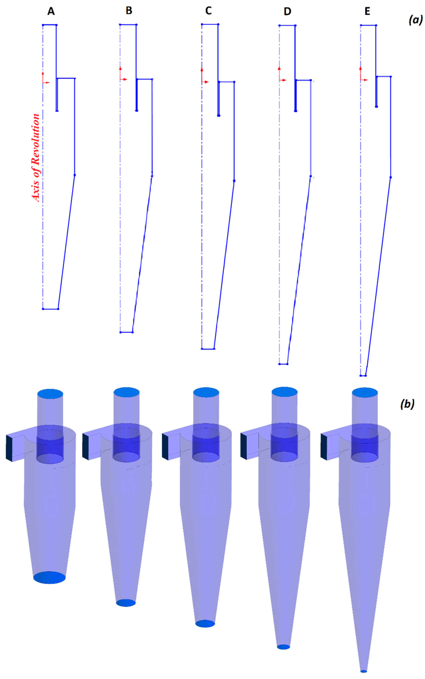
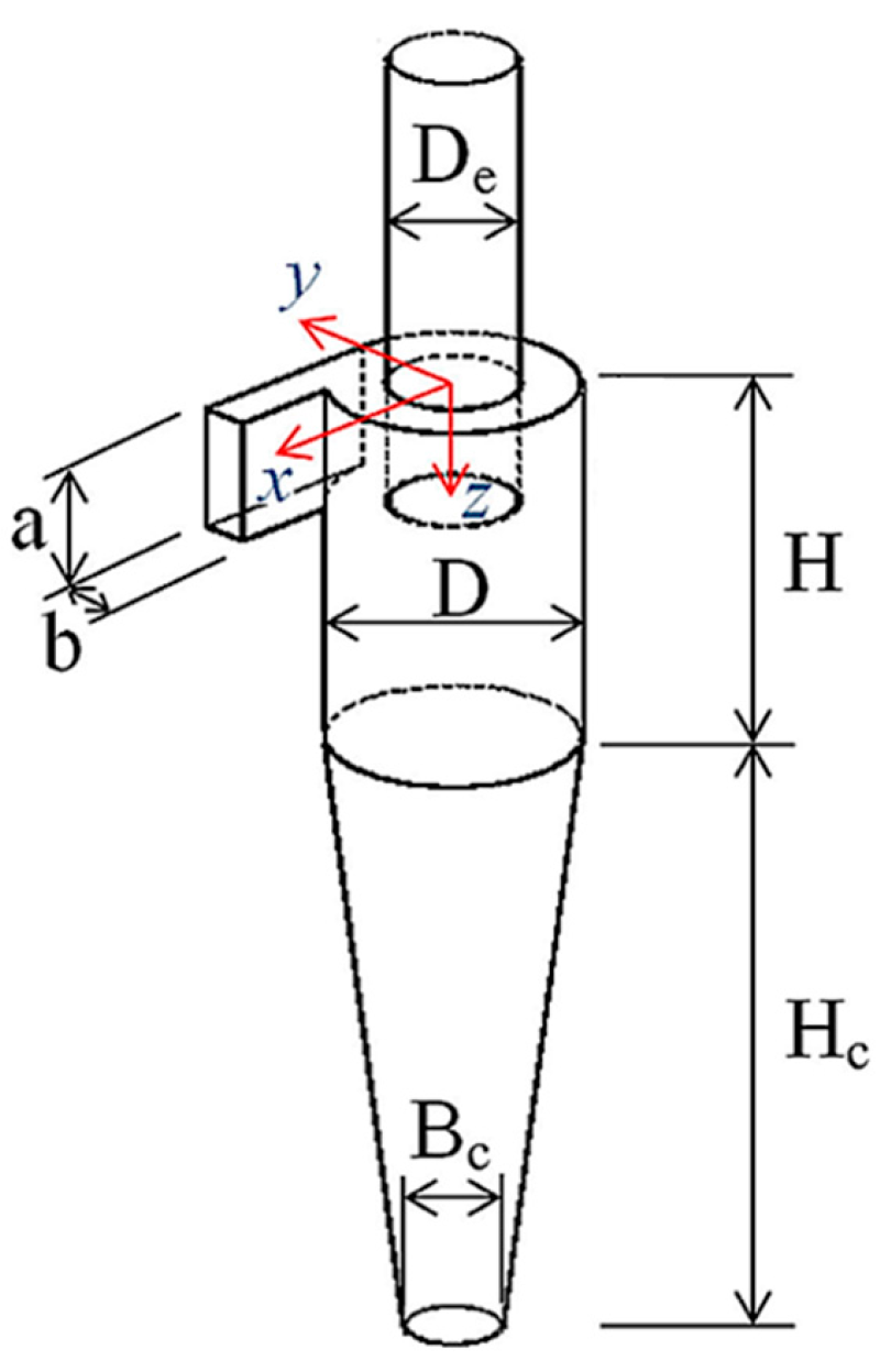
3.1. The Details of Cyclone Geometry

A Stairmand high-efficiency cyclone [30] was considered for analysis. It consists of a cylinder-on-cone configuration with a tangential inlet. The schematic is presented in Figure 1, and the concerning dimensions are given in

Table 1. Dimensions of the cyclone model.

Cyclone Geometry	Cyclone Model	Symbols (Normalized with D)	Dimensions [-]
Vortex finder diameter		De/D	0.5
Inlet duct height		a/D	0.5
Inlet duct width		b/D	0.2
Vortex finder insertion length		Lv/D	0.5
Height of cylindrical section		H/D	1.5
Height of conical segment	A	Hc/D	1.5
	B		2.0
	C		2.5
	D		3.0
	E		3.5
Cone-tip diameter	A	Bc/D	0.3125
	B		0.2500
	C		0.1875
	D		0.1250
	E		0.0625

. The main body diameter (D) was taken as 0.29 m for all the models. As mentioned earlier, we considered elongation of the conical segment such that the apex cone angle remained the same in all cases. Thus, increasing the cone length (H_c) also influenced the bottom opening (B_c). For instance, increasing the cone length value (H_c/D) from 1.5 to 3.5 reduced the bottom opening value (B_c/D) from 0.3125 to 0.0625. The details have been provided in Table 1. Hence, the cyclone performance was an interaction of the two geometrical entities viz. the cone length and cone tip diameter. A complete detail of all the cyclone models is represented as a 2-D sketch in Figure 2a and the respective 3-D geometry is shown in Figure 2b.

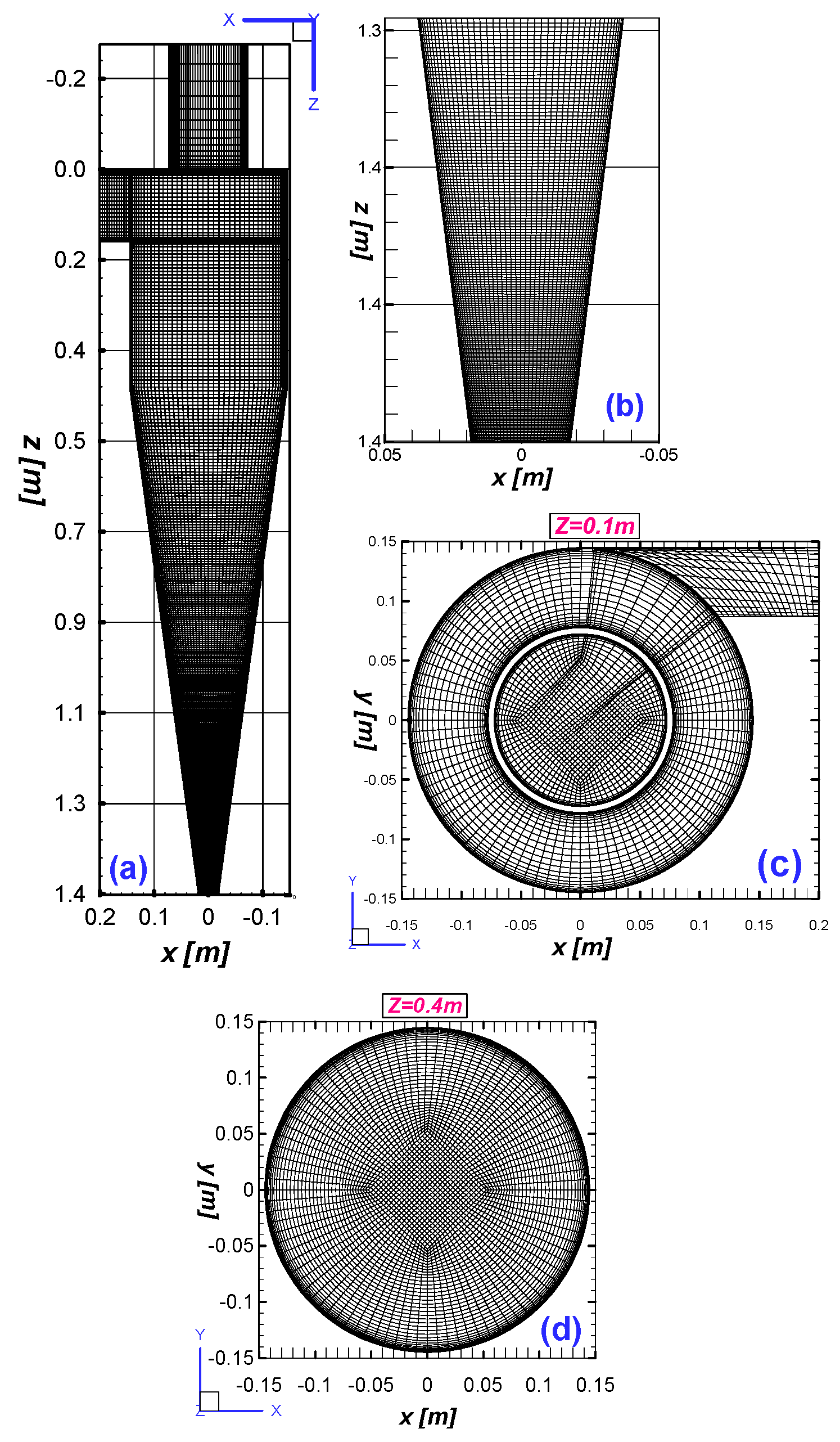
3.2. Mesh Generation

Meshing is considered a key component in the pre-processing of CFD. Here, the domain of the fluid was meshed with hexahedral elements using ICEM CFD. The multi-blocking strategy was considered here, since it gives complete control over the mesh density and also aids the local grid refinement. The mesh was refined in the core region and near the walls to accurately capture the flow physics. Furthermore, the alignment of the cells along the curved flow streamlines was ensured to reduce the numerical diffusion. Figure 3 represents the details of the mesh in model E over different planes as well as surfaces. To accurately capture the flow phenomenon and the particle trajectories—especially in the lower part of the cyclone—the conical segment was highly refined.

Table 2. Mesh count (in millions) for cyclones with different model.

Model	A	B	C	D	E
Mesh count	0.685 M	0.880 M	1.5 M	1.6 M	1.8 M

illustrates the details of the mesh count for all the cyclone models.

3.3. CFD Methodology

Air was taken as the continuous phase in the simulation, and the particles were considered as a discrete phase. One-way coupling was considered for low-dust conditions (less than 10% by volume). The evaluation of the continuous phase relied on analyzing the governing equation over the control volumes fixed in space, while discrete phase tracking required the Lagrangian approach. Consequently, the Eulerian–Lagrangian approach was utilized to completely model the cyclonic flows.

The RNG k-ε model was used to set up the initial (steady state) flow field. For the near-wall condition, a standard wall function was considered. A solver tolerance equal to 10⁻⁵ was used for the conservation equations. The developed field served as the starting point for the LES simulations, saving a considerable amount of effort and time. The LES simulations were carried out until the monitored flow variables reached a (quasi) steady state. The collection efficiency was then determined by the number of particles being retained in cyclones.

3.4. Numerical Settings and Boundary Conditions

3.4.1. Continuous Phase

The air of density equal to 1.1 kg/m³ and viscosity of 1.834 ∙ 10⁻⁵ kg/m·s was considered as a working medium for the continuous phase. A uniform profile of a velocity inlet boundary condition was provided at the inlet. The inlet velocity was taken as U_in = 10 m/s, 15 m/s, and 20 m/s, resulting in Reynolds numbers Re = 1.23 ∙ 10⁵, 1.84 ∙ 10⁵, and 2.45 ∙ 10⁵. The pressure outlet boundary condition was considered at the outlet of the cyclone. A no-slip boundary state was allotted for the respective boundaries, and the Smagorinsky constant C_s = 0.1 was utilized for modeling the sub-grid scales. As discussed in the earlier section, a 0.1 ms time step size was applied for the simulation of all numerical models.

In the present work, the least-squares cell-based method was utilized to calculate the cell gradients. To interpolate the pressure values at the cell faces, we used the PRESTO! (PREssure Staggering Option) scheme, as it is suitable for highly anisotropic swirling flows. To discretize the diffusion terms in momentum transport equations, we used the second-order bounded central differencing scheme. The fractional step scheme with the NITA (non-iterative time advancement) algorithm was coupled with pressure and velocity for the LES turbulence model. Although NITA requires a large amount of memory, significant time can be saved compared to iterative time advancement. For the time enhancement, a bounded second-order implicit scheme, and for the momentum, a bounded central differencing scheme were used. The stated numerical settings have already been utilized by several authors [3,4,7,10,14,17,18,23].

3.4.2. Discrete Phase

A total of 30,160 solid particles, having a density of 2800 kg/m³, were injected into the cyclone model in the face-normal direction. Ten different particle diameters ranging from 0.5 μm to 10 μm were considered. A time-step size equivalent to that of a continuous phase, i.e., 0.1 ms, was used. All the simulations were performed at three inlet velocities viz. 10 m/s, 15 m/s, and 20 m/s. The particles reaching the bottom plate of the cyclone were considered trapped. Hence, a trap boundary condition was applied at the bottom plate. The outlet plane was assigned as the escape boundary condition. For the remaining boundary walls, a rebound boundary condition was applied, and the coefficient of restitution was taken as unity for both wall-normal and tangential directions. Therefore, the solid particles reaching these surfaces rebounded without any losses. Several studies have already utilized these boundary conditions [7,9,10,17,18,24].

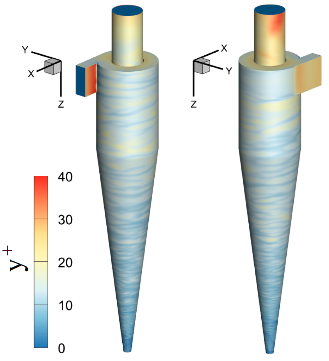
3.4.3. Near-Wall Treatment

Special consideration is required for simulating the wall-bounded flows due to the existence of the large velocity gradients in the direction parallel to the wall as well as in the wall-normal direction. Since the standard Smagorinsky subgrid model was chosen, a wall-damping function was required near the wall to reduce the eddy viscosity to zero. Hence, we used ${\mu }_{sgs}=\rho l_{sgs}^2\left|S\right|$, where ρ is the fluid density, l_sgs denotes the subgrid scale mixing length, and $\left|S\right|=\sqrt{2{\overline{S}}_{ij}{\overline{S}}_{ij}}$ is the resolved deformation rate [30]. A similar approach was used in several prior studies [7,31,32].

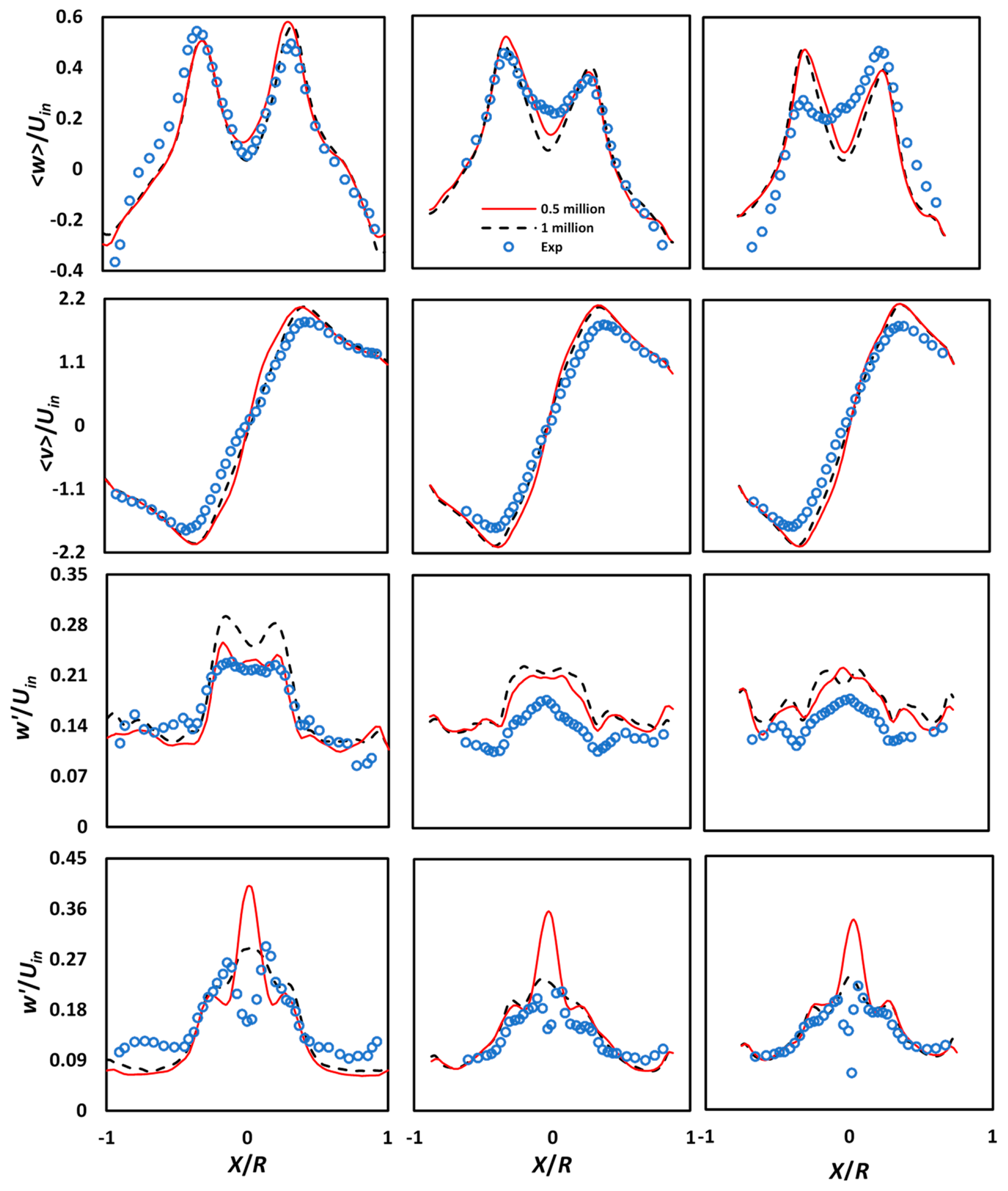
3.5. Validation and Methodology

Before performing a CFD analysis, the approach must be validated with available experimental data for both continuous and discrete phases. The grid was tested at two levels viz. 0.5 million cells (coarse grid) and 1.0 million cells (fine grid). The numerically calculated average root mean square error (rmse) values of axial and tangential velocity at different locations viz. Z/D = 0.75, 2.0, and 2.5 were compared with the experimental data of Hoekstra [2], in which the Stairmand cyclone with a body diameter of 0.29 m was used. Two levels of mesh have been used, the details of which are provided in

Table 3. Mesh count for cyclones used in validation.

	LES (Coarse)	LES (Fine)
Mesh count	0.5 million	1.0 million

.

Using LES, the numerically generated mean and fluctuating values of the tangential and axial components are compared with that of the reference model [2] at Reynolds number (Re) = 2.8 ∙ 10⁵. Two levels of the grid have been evaluated. The average values of the axial and tangential velocity components are shown in the first and second rows of Figure 4. Differences in results between grid levels are minimal, indicating that the solution is grid independent. Moreover, the coarse and fine mesh results agree very well with the experimental data. However, the coarse mesh results at Z/D = 1.0 showed the smallest deviation in the mean axial velocity, whereas at Z/D = 2.0 and Z/D = 2.5, the local dip near the axis overshot moderately. The third and fourth lines of Figure 4 represent the rmse values of the axial and tangential velocities, respectively. A good agreement between the rmse values and experimental data was observed, particularly in the outer vortex region. However, in the core region, a mild increase in the rmse axial velocity was observed. It becomes apparent from the last row of Figure 4 that the nature of rmse tangential velocity was different from the reference data near the central axis of the cyclone, whereas the former exhibits a local shoot-up rather than a dip. The mesh refinement could be responsible for the small errors (e.g., in the mean velocity profiles) getting amplified in the precession-induced fluctuation levels. Such discrepancies in the mean and rmse velocity profiles have also been reported in several previous studies [33,34,35]. Hence, despite the known issues with resolving the flow anisotropy using advanced closure LES, the simulation procedure may be applied to all future simulations.

4. Results and Discussion

In this section, we present the details of the flow field viz. mean and fluctuating velocity as well as pressure over the cut planes followed by the radial profiles at different axial locations. This is accompanied by a detailed discussion on the dynamic nature of the vortex core that precesses about the geometrical axis and produces coherent fluctuations. Finally, we discuss the impact of increasing the cone length and inlet velocity on the pressure drop and collection efficiency of cyclones.

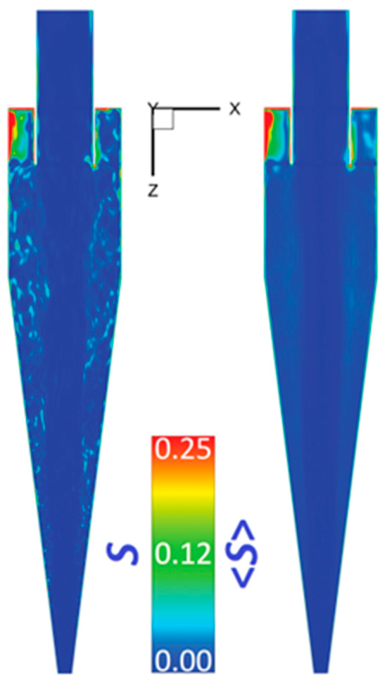
4.1. The Quality of LES

The motivation to use LES was to directly resolve a large part of the flow (preferably, more than 80%) [36] to keep the contributions from the SGS modeling to a minimum. Prior to the discussion of the scalar and vector fields, we accessed the quality of LES. We perform a check for the unresolved part, calculated as a fraction (S) of the SGS turbulent kinetic energy (TKE) to the total TKE (defined as the sum of TKE contributions from both resolved as well as unresolved parts), i.e.,

$$\mathit{S}=\frac{{\mathit{k}}_{\mathit{S}\mathit{G}\mathit{S}}}{{\mathit{k}}_{\mathit{S}\mathit{G}\mathit{S}}+{\mathit{k}}_{\mathit{r}\mathit{e}\mathit{s}}}$$

(23)

Here, the SGS TKE is calculated as

$${\mathit{k}}_{\mathit{s}\mathit{g}\mathit{s}}={\left(\frac{{\mathit{\nu }}_{\mathit{s}\mathit{g}\mathit{s}}}{\mathsf{\rho }·{\mathit{l}}_{\mathit{s}\mathit{g}\mathit{s}}}\right)}^{\mathbf{2}}$$

(24)

and the resolved scale SGS is taken as

$${\mathit{k}}_{\mathit{r}\mathit{e}\mathit{s}}=\frac{\mathbf{1}}{\mathbf{2}} [\mathit{u}{\prime }^{\mathbf{2}}+\mathit{v}{\prime }^{\mathbf{2}}+\mathit{w}{\prime }^{\mathbf{2}}]$$

(25)

where u′, v′, and w′ are the root mean square error terms of velocity components in the x-, y-, and z-directions, respectively.

When using the standard Smagorinsky SGS model, the subgrid length scale is calculated as

$${\mathit{l}}_{\mathit{s}\mathit{g}\mathit{s}}=\mathit{m}\mathit{i}\mathit{n} \left(\mathit{k}·\mathit{d}, {\mathit{C}}_{\mathit{s}}·\Delta \right)$$

(26)

where kappa is the von Karman constant given as k = 0.41, d is the closest wall distance, C_s is the Smagorinsky constant (taken as 0.1), and Δ is the filter size, which is equal to the cubic root of the cell volume (i.e., V^1/3; V is the local cell volume).

Here, to calculate the contributions of TKE from the SGS model, we calculate the length scale from Equation (26) as $l_{sgs}=C_s·\Delta$.

Clearly, this expression is valid for the entire domain other than the walls. However, regarding the details near the walls, a brief discussion on y⁺ values is warranted. Figure 5 represents the TKE from the SGS model implemented in LES; both the instantaneous (to the left) and mean (to the right) values of S are represented. The latter is calculated as

$$<\mathit{S}>=\frac{<{\mathit{k}}_{\mathit{S}\mathit{G}\mathit{S}}>}{<{\mathit{k}}_{\mathit{S}\mathit{G}\mathit{S}}>+<{\mathit{k}}_{\mathit{r}\mathit{e}\mathit{s}}>}$$

(27)

The symbol (<·>) denotes the mean values.

It becomes apparent that a major part in the flow regime is well-resolved, whereas the contribution from the SGS models is very small and limited only to the annular region close to the inlet duct. The same is demonstrated by both the instantaneous as well as means values of S in Figure 5. Since the grid in all the parts of the cyclone, other than in the conical section along the z-direction, is identical, the same holds for all the models. Hence, the results for cyclone model E alone are presented here.

The first cell height that is adjacent to the solid boundaries plays an important role in the accuracy of the results. The centroid of the first cell near the solid wall falls within the log-law regime, and the solver applies the law-of-the-wall approach. Here, as mentioned earlier, we present the y⁺ values (cf. Figure 6) only for cyclone variant E. It becomes apparent that the global y⁺ value does not exceed 40, which indicates a fair figure with the wall-modeling approach.

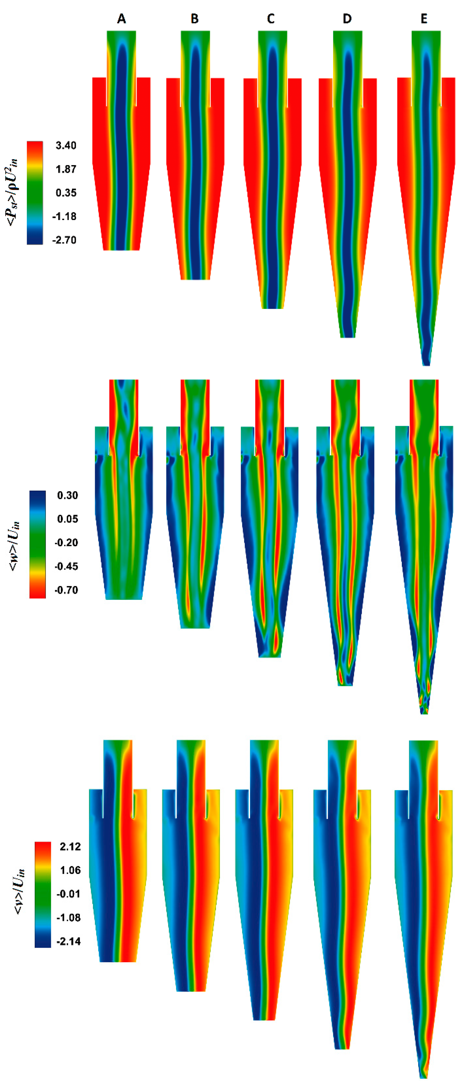
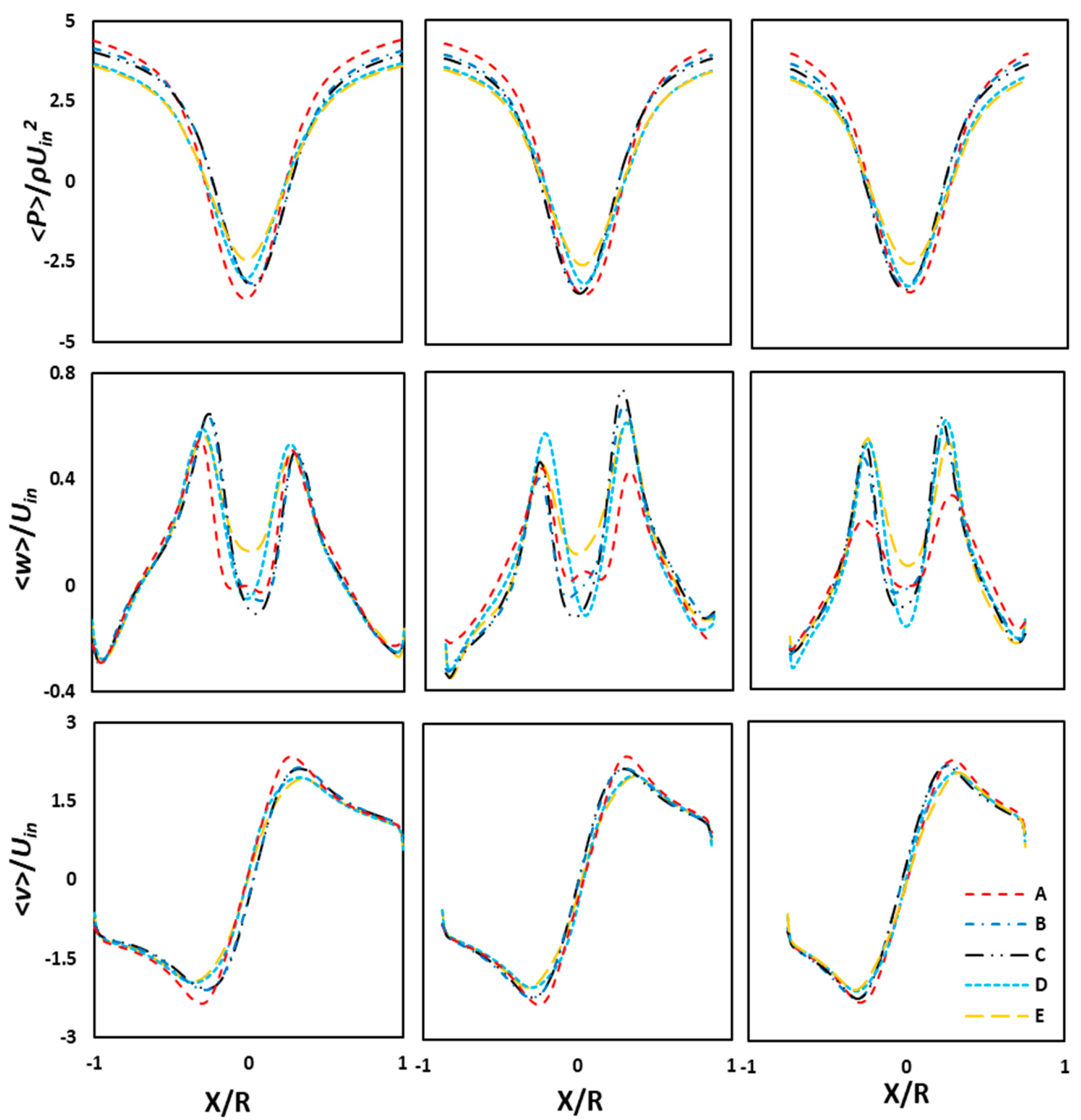
4.2. The Mean Flow Field

The contour plots of the time-averaged static pressure, tangential velocity, and axial velocity in all the cyclone models are shown in Figure 7, and their respective radial profiles at three cut sections along the cyclone axis (Z/D = 1.0, 2.0, and 3.0) are presented in Figure 8. The pressure distribution is almost identical in all the models. In the core region, we noticed a negative pressure region, which meant that the pressure dropped below the atmospheric pressure. The static pressure was at maximum in the outer region near the solid walls, and this value reduced significantly as we moved toward the center. The wall static pressure was at maximum in model A, at minimum in model E, and intermediate in models B–D. The cyclone models having larger wall static pressure values in general indicate higher pressure losses.

From the second row in Figure 7, it is apparent that the axial velocity had two flow streams. The outer vortex was directed towards the cyclone bottom, and the inner vortex was oppositely directed towards the outlet, i.e., the vortex finder exit. The same is also reflected in the second row of Figure 8, which illustrates the radial profiles at different locations. The downward directed flow had the largest magnitude near the outer walls, and it reduced when moving radially inward, until its value became zero at the radial location. Thereafter, the axial velocity took the positive values in the remaining region, indicating upward direction flow. The variations in the outer vortex were very mild in all models at all axial locations. However, in the core region, the variations were quite large, particularly in the conical segment: a large variation can be seen at Z/D = 3.0. Cyclone model C had the maximum value in the upward direction, and model A had the lowest one.

As can be seen in the third row of Figure 7 and Figure 8, the maximum tangential velocity was approximately twice as large as the inlet velocity and was constant along the cyclone axis. In the core region, the tangential velocity varied linearly, i.e., it was zero in the rotational axis of the inner vortex and increased linearly in the core region until it reached the maximum value. Thereafter, the tangential velocity magnitude decreased rapidly in a non-linear manner and reduced significantly near the outer walls. The slope of the tangential velocity was almost the same for all the models, but the peak values had mild variations. The region confined to the inner vortex was hardly affected. The peak value of the tangential velocity was larger in model A and at minimum in model E. Furthermore, the magnitude of the tangential velocity decreased from model A–E. Interestingly, with an increase in the length of the cone, the frictional losses, although smaller, as apparent from the marginal reduction in the peak value of tangential velocity, were still relevant. However, in a study by Brar et al. [17] (cf. Figure 9, p. 674), wherein the cone angle increased with an increase in the cone length, the decay in the tangential velocity was larger than in the present study. This means that the cone angle plays a vital role in cyclones with longer heights.

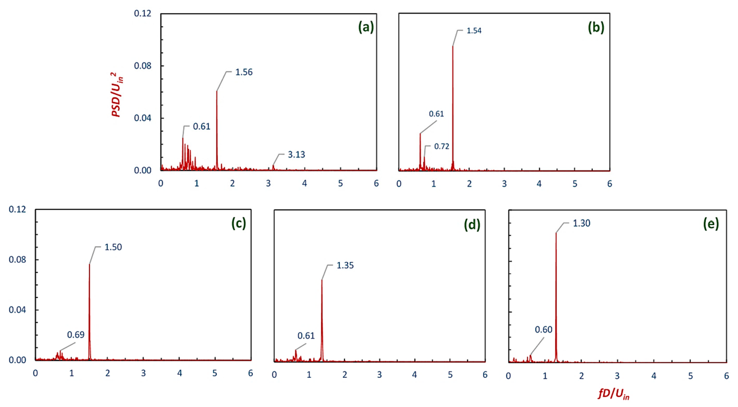
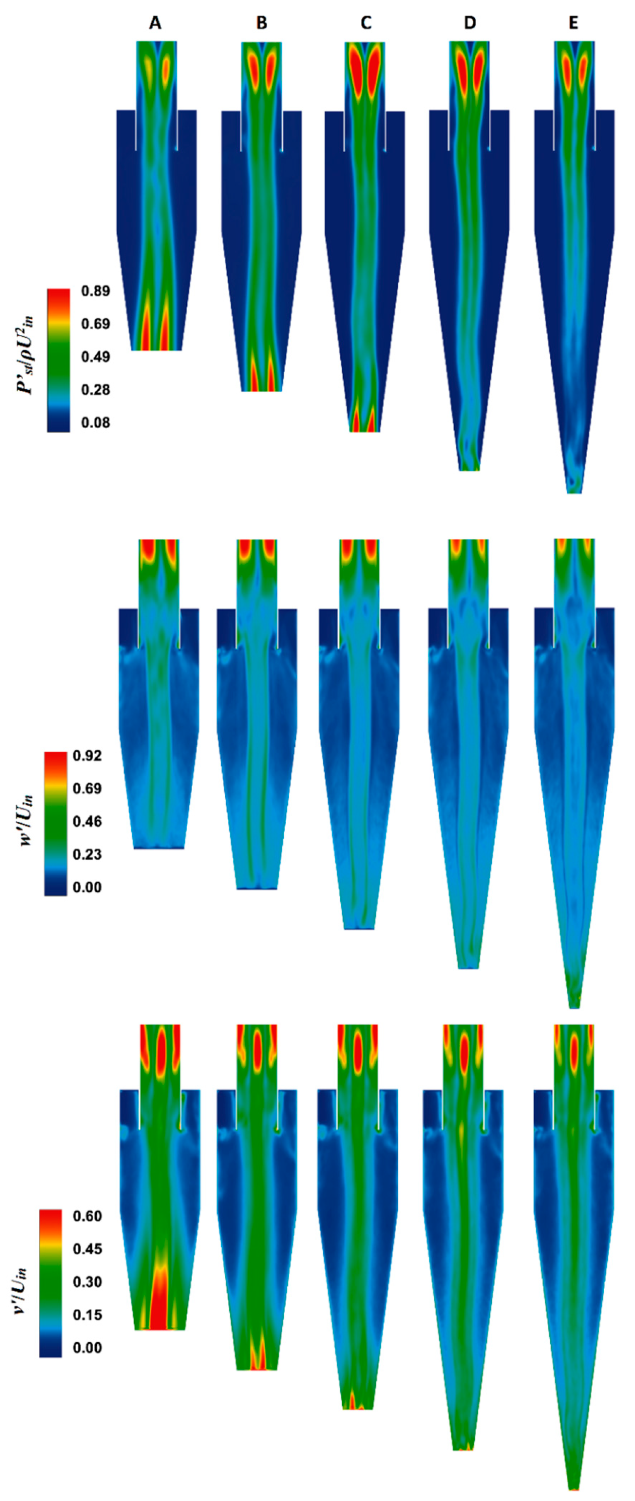
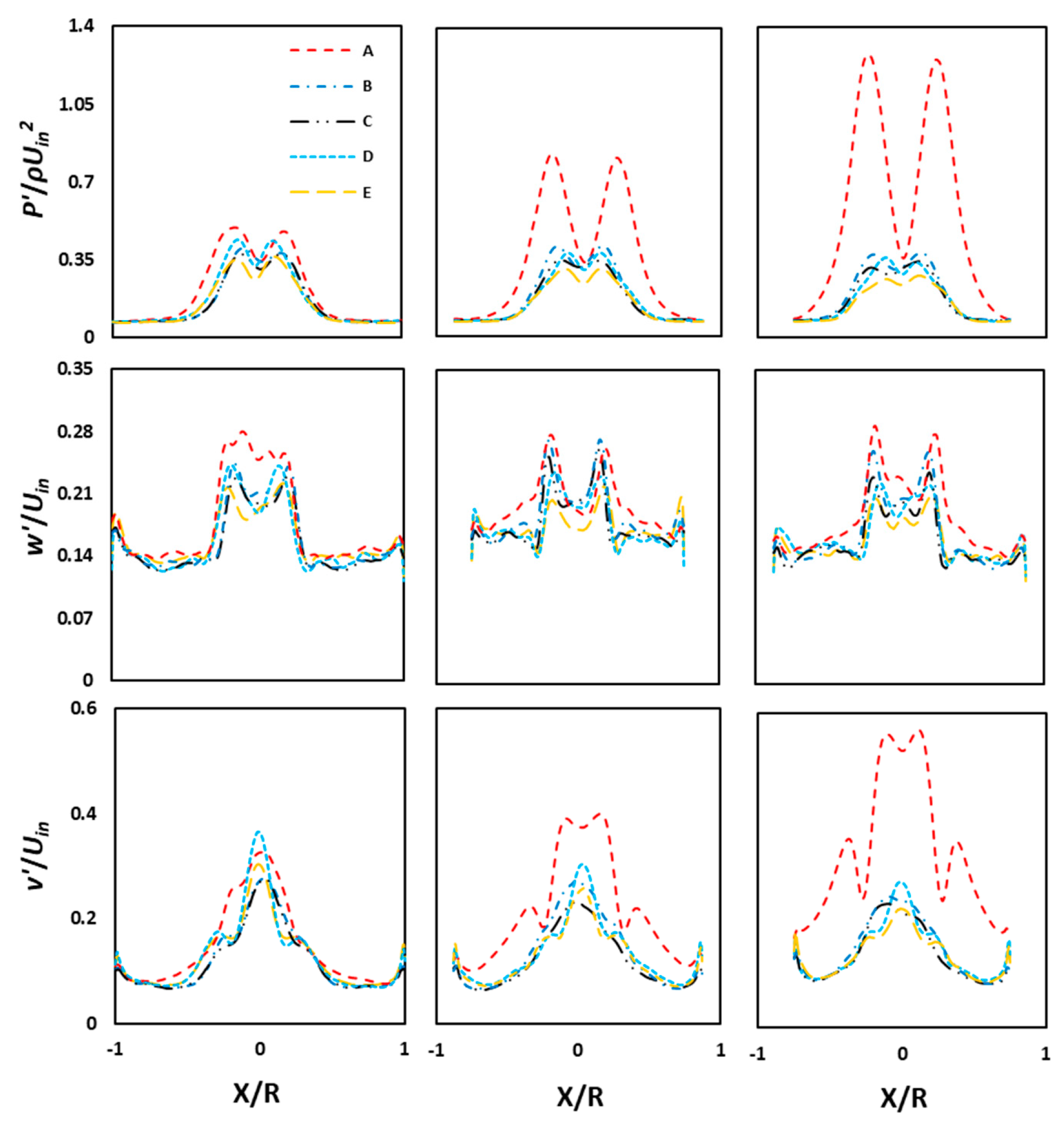
4.3. The Fluctuating Flow Field

Cyclonic flows encounter coherent fluctuations in the core region, accompanied by weak turbulent fluctuations in the outer vortex regime [37]. These fluctuations are mainly responsible for particle dispersion near the wall. In the present work, the fluctuations are represented by root mean square error (rmse) values. The contour plots and the radial profiles are shown in Figure 9 and Figure 10, respectively. The first, second, and third rows represent, respectively, the static pressure fluctuations, the axial velocity fluctuations, and tangential velocity fluctuations. It is apparent that the pressure as well as the axial and tangential velocity components exhibit a significantly higher level of fluctuations in the core region than in the outer vortex region. These fluctuations, in the vortex core region of the cyclone, take place due to the precessing of the rope-like coherent structure about the geometrical axis. In the outer vortex, the (weak) turbulent fluctuations that have the least contributions from the (strong) coherent fluctuations persist. Two important observations here are that (a) the pressure and velocity fluctuations reduce with an increase in the cone length, and (b) the tangential velocity fluctuations are much stronger than the axial velocity fluctuations. Figure 10 shows the radial plots of rmse values of scalar and vector fields, wherein the fluctuation levels are much higher close to the bottom of the cyclone and near the exit plane. The latter arises due to the movement of the vortex core end near the edge of the outlet plane. Interestingly, the level of fluctuations at the cyclone bottom surface is much larger in model A and lowest in model E. This is due to the fact that the larger bottom plane diameter (such as in model A) serves more space for the lateral movement of the precessing vortex core end on that plane, and this freedom to precess over a narrow plane is highly restricted (such as in model E). A similar observation holds in the radial plots of rmse values in Figure 10. The tangential velocity fluctuations are larger in model C, followed by model D. For other models, these values decrease with an increase in the cone length. At a given station, the complex variations in different models are due to the combined effect of the contracting conical region at the lower end and the elongation of the cone. In other words, the inner vortex experiences an elongation in length, followed by lateral contraction with an increase in cone length.

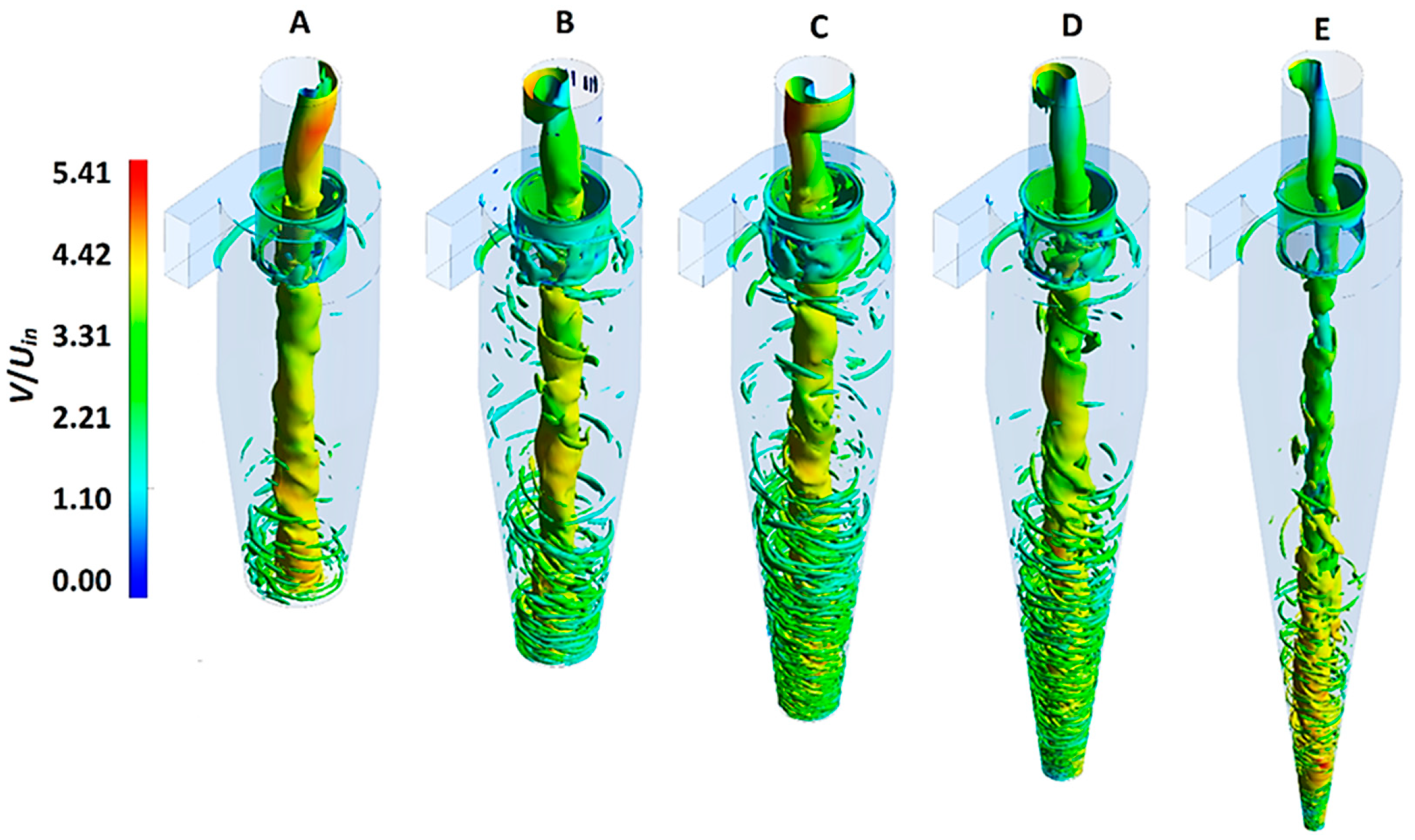
4.4. The Representation of the Vortex Core

When the axis of the swirling coherent structure gets displaced from the geometric centerline and starts precessing about it, the phenomenon is termed a precession vortex core (PVC). The frequency of the PVC is considered an important factor and is generally governed by the cyclone geometry and the operating conditions [38]. Figure 11 represents the vortex core representation based on the λ₂ criterion. The vortex core resembles a twisted rope-like structure extending throughout the cyclone length. The λ₂ criterion represents the coherent structures based upon the iso-surface values: at different values, eddies with different length scales appear. However, we selected a value of 0.35, which was found to be a good balance for the visualization of the vortex core. Interestingly, in the core region, the diameter of the coherent structure seemingly reduces from models A–E.

It has been reported that correlations exist between the PVC and the tangential velocity as well as pressure values [35]. In Figure 8, it becomes apparent that the magnitude of mean tangential velocity as well as mean wall static pressure decreases mildly from model A to E. The same trend of (a mild) reduction in the frequency values is reflected in the frequency plot; interestingly, this is in close agreement with another study [35].

The PVC is a mechanism that shows certain irregularities viz. phase jump and non-uniform amplitudes [37]. To identify the periodicity, Fast Fourier Transformation (FFT) was applied over the time-dependent variables. Here, the tangential velocity signal was recorded at a point (X/D = Y/D = Z/D = 0). Figure 12a–e shows the power spectral density (PSD) plots, normalized with the square of the inlet velocity, for all the cyclone models A–E, respectively. The frequency is represented in dimensionless form as a Strouhal number, given as St = fD/U_in, with f, the frequency (in Hz); D, the cyclone main body diameter (in m); and U_in, the inlet velocity (in m/s). Multiple peaks with a very low power were observed in the frequency range of 0 to 50 Hz in nearly all the models. However, in the frequency band ranging from 50 to 100 Hz, a prominent spectral peak was observed that corresponds to the principal frequency of the flow system. The power related to the lower harmonic is considerably less than the higher harmonic in cyclone model E. For cyclones A–E, the corresponding frequencies of the lower harmonic were calculated as St₁ = 0.61, 0.61, 0.69, 0.61, 0.61, and 0.60, whereas the frequency of the higher harmonic in cyclones from models A–E was calculated as St₂ = 1.56, 1.54, 1.50, 1.35, and 1.30, respectively. Interestingly, the principal frequency reduced with an increase in the cone length for all inlet velocities, as represented in Figure 13.

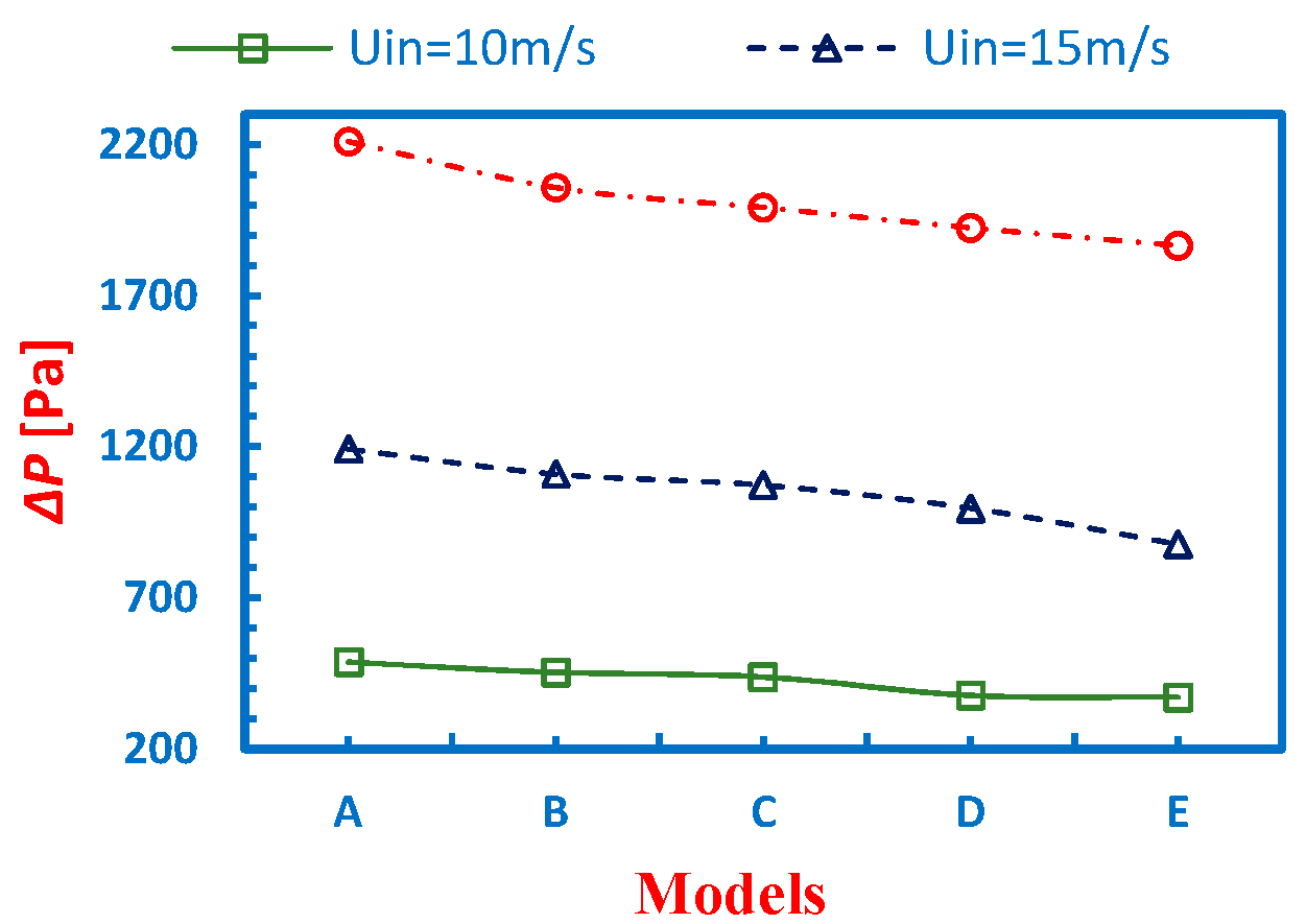
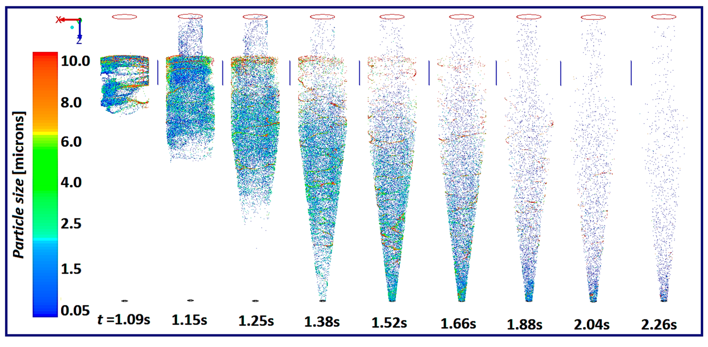
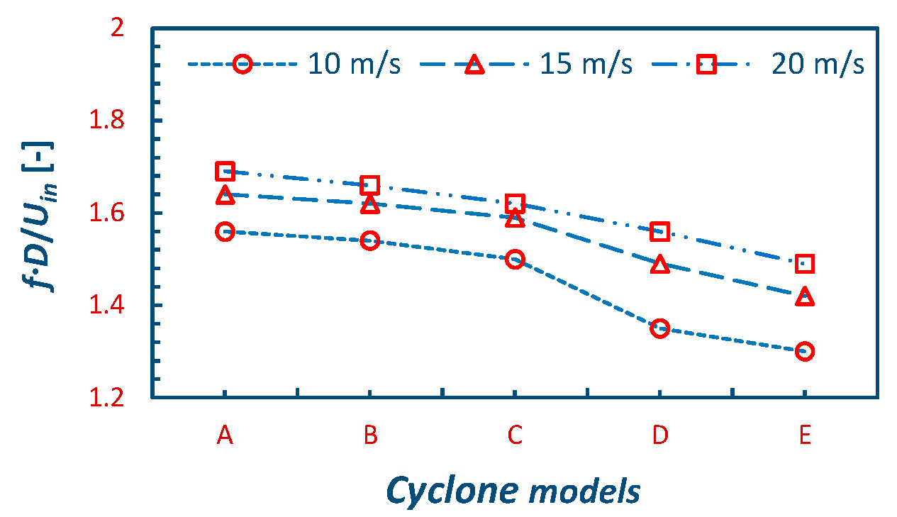
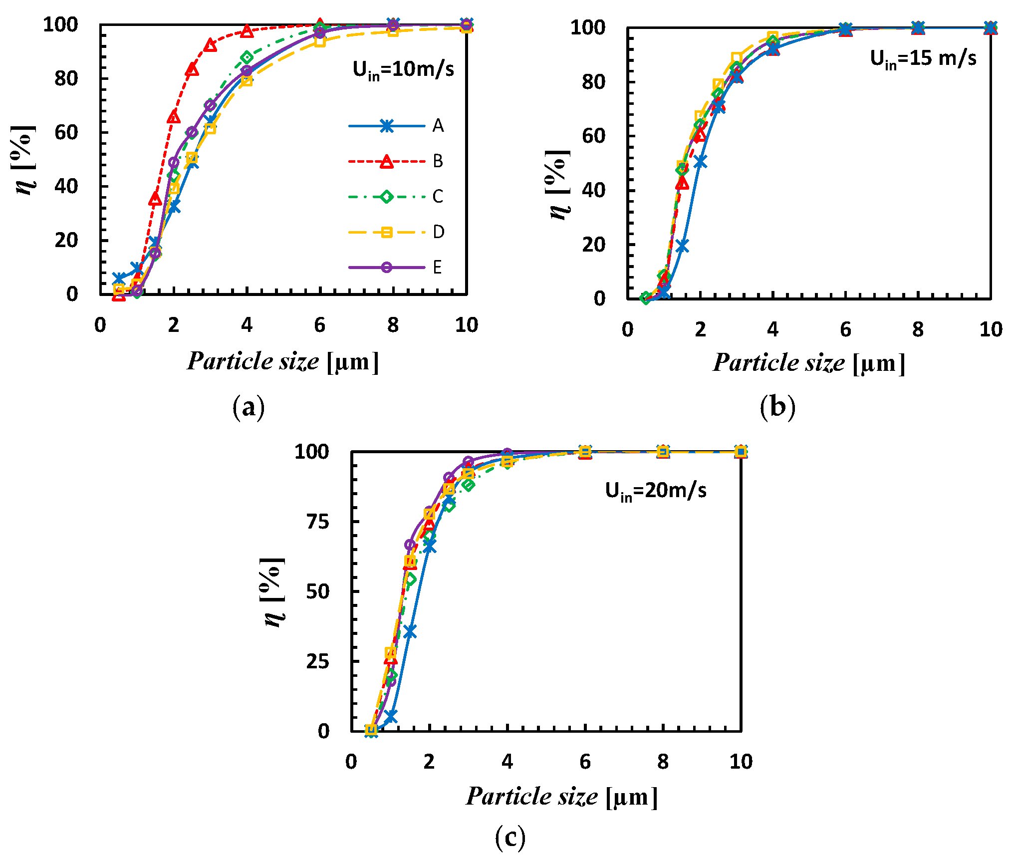
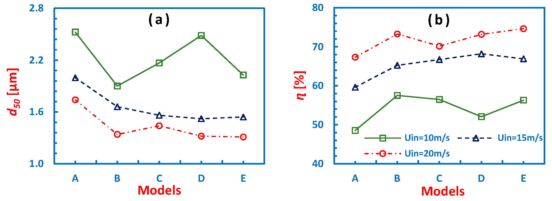
4.5. Performance of the Cyclone

The performance of the cyclone is determined by the pressure drop values (ΔP), collection efficiencies (η), and cut-off diameters (d₅₀). The pressure drop is defined as the difference in total pressure values across the inlet and outlet, while the cut-off diameter is the particle size that corresponds to 50% collection efficiency on the grade efficiency curve (GEC) curve. The separation efficiency is the ratio of the number of particles retained by the cyclone separator to the number of particles injected at the inlet of the cyclone separator. In cyclone separators, the pressure losses are known to take place mainly inside the vortex finder tube due to a high swirl intensity of the fluid leaving the cyclone, followed by the losses at the walls as well as due to fluid friction. Furthermore, due to a nonlinear increase in the tangential velocity peak values and a significant increase in the velocity fluctuations, the pressure losses increase significantly with an increase in Re [14].

The pressure drop values in all cyclone models, for all inlet velocities, are represented in Figure 14. It was found that as the inlet velocity is increased, the pressure drop increases significantly in each model. At a given inlet velocity, the maximum pressure drop was found in model A and its magnitude decreases as the cone height is increased. This is due to the fact that the magnitude of tangential velocity reduces with increasing cone length. It is important to note that this velocity component governs the strength of the swirling fluid and dictates the pressure losses and also the collection efficiency in cyclone separators.

Figure 15 shows GECs for all the models operating at different inlet velocities. Surprisingly, a gradual shift in the GECs is not observed with increasing cone length despite a reduction in the peak values of tangential velocity. Figure 16a summarizes the cut-off values at different inlet velocities. It becomes apparent that only at 15 m/s, the d₅₀ values reduce consistently with length, whereas at the lower and upper values of inlet velocities, the results are dramatic. It is observed that at 10 and 20 m/s, the lowest d₅₀ value exists for cyclone model B, and for all U_in, d₅₀ is the largest for model A. Figure 16b illustrates the total collection efficiency for all models at different U_in. At the lower and upper limits of velocity, cyclone model B has the highest value of η, whereas cyclone model A has the lowest value of η. However, Brar et al. [17] reported a consistent reduction in d₅₀, and an increase in η with an increase in the cone length (cf. Figure 13, p. 675; and Figure 15 p. 676). The difference in the results is due to the fact that in the present study, given that the apex cone angle is held fixed, the cone tip (a lower bottom opening) undergoes a significant reduction in the diameter with an increase in the length of the conical segment, whereas in another study [17], the cone-tip diameter remained the same for each increment in the cone length. There is a contradictory nature in the mean tangential velocity and the velocity fluctuation fields: the former acts as a source of centrifuging the solid particles towards the outer walls, while the latter has a strong tendency to disperse these particles (which causes a reduction in the collection efficiency) [39]. Hence, the variations in the collection efficiency and cut-off particle size are due to the combined effect of the mean as well as the fluctuating flow field, particularly in the lower part of the cyclone, where a large variation in the latter exists (cf. Figure 9).

Therefore, it becomes apparent that the cone-tip diameter and the apex angle of the cone become important parameters that significantly influence the collection efficiency in cyclones with longer cone lengths. Therefore, the present work provides important guidelines for considering the cone-tip diameter when increasing the cone length.

The trajectories of the particles of different sizes are shown in Figure 17. Seemingly, the larger particles have a greater tendency to move out towards the outer walls and stay close to the walls throughout their movement. The lighter particles, on the other hand, experience larger drag force due to smaller size, and the velocity fluctuations further disturb the trajectories of these particles. Hence, smaller particles are easily carried away by the fluid leaving the cyclone separator through the outlet tube.

5. Conclusions

A numerical study was undertaken on a Stairmand high-efficiency cyclone with increasing conical lengths to evaluate their impact on the pressure drop and collection efficiency. For this, the advanced closure model LES was used with the standard Smagorinsky SGS model to predict the mean as well as the fluctuating component of the velocity. This was followed by a calculation of the cyclone performance. The frequency with which the vortex core precesses was also determined. We found that the numerical simulations were in good agreement with the experimental data. For analysis, five cyclone models were proposed with increasing heights of the conical section and decreasing diameter of the cone tip, referred to as cyclone models A, B, C, D, and E, respectively. The performance parameters of these cyclone models were determined. Conclusive results indicate the following:

• The pressure drop decreases by increasing the conical height of the cyclone separator and decreasing the cone-tip diameter.
• The magnitude of the tangential velocity decreases as the length of the cyclone separator increases along with the diameter of the cone tip.
• The velocity fluctuations were suppressed in models A–E.
• The frequency with which the vortex core precesses about the geometrical axis was lowest in model A and it decreased gradually from cyclone models A–E.

Quantitatively, with increase in the cone length from A to E at Re = 1.84 ∙ 10⁵, the following was observed:

• The pressure drop reduced from 1017 Pa to 877 Pa.
• The collection efficiency increased from 59.63% to 63.90%.
• The cut-off size reduced from 2 μm to 1.54 μm.

This study provides guidelines for considering the cone-tip size (and thus the apex angle of the cone) when increasing the cone length in cyclones.

It is worthwhile to mention here that we assumed a one-way coupling approach, and the particles were assumed to be spherical in shape. In future work, non-spherical particles may be tested using a two-way coupling approach, which would permit influence due to the interaction between both phases.

References

1. Flagan, R.C.; Seinfeld, J.H. Fundamentals of Air Pollution Engineering; Prentice-Hall, Inc.: Englewood Cliffs, NJ, USA, 1988; ISBN 0-13-332537-7. Available online: http://resolver.caltech.edu/CaltechBOOK:1988.001 (accessed on 25 November 2022).
2. Hoekstra, A.J. Gas Flow Field and Collection Efficiency of Cyclone Separators. Ph.D. Thesis, Technical University Delft, Delft, The Netherlands, 2000. Available online: http://resolver.tudelft.nl/uuid:67b8f405-eef0-4c2d-9646-80200e5274c6 (accessed on 2 May 2022).
3. Ficici, F.; Ari, V. The influence of diameter of vortex finder on cyclone collection efficiency. Environ. Prog. Sustain. Energy 2014, 34, 669–673. [Google Scholar] [CrossRef]
4. Wasilewski, M.; Brar, L.S.; Ligus, G. Experimental and numerical investigation on the performance of square cyclones with different vortex finder configurations. Sep. Purif. Technol. 2020, 239, 116588. [Google Scholar] [CrossRef]
5. Elsayed, K. Design of a novel gas cyclone vortex finder using the adjoint method. Sep. Purif. Technol. 2015, 142, 274–286. [Google Scholar] [CrossRef]
6. Parvaz, F.; Hosseini, S.H.; Ahmadi, G.; Elsayed, K. Impacts of the vortex finder eccentricity on the flow pattern and performance of a gas cyclone. Sep. Purif. Technol. 2017, 187, 1–13. [Google Scholar] [CrossRef]
7. Brar, L.S.; Elsayed, K. Analysis and optimization of cyclone separators with eccentric vortex finders using large eddy simulation and artificial neural network. Sep. Purif. Technol. 2018, 207, 269–283. [Google Scholar] [CrossRef]
8. Elsayed, K.; Lacor, C. The effect of cyclone inlet dimensions on the flow pattern and performance. Appl. Math. Model. 2011, 35, 1952–1968. [Google Scholar] [CrossRef] [Green Version]
9. Wasilewski, M.; Brar, L.S. Effect of the inlet duct angle on the performance of cyclone separators. Sep. Purif. Technol. 2019, 213, 19–33. [Google Scholar] [CrossRef]
10. Yoshida, H.; Ono, K.; Fukui, K. The effect of a new method of fluid flow control on submicron particle classification in gas-cyclones. Powder Technol. 2005, 149, 139–147. [Google Scholar] [CrossRef]
11. Bernardo, S.; Mori, M.; Peres, A.; Dionísio, R. 3-D computational fluid dynamics for gas and gas-particle flows in a cyclone with different inlet section angles. Powder Technol. 2006, 162, 190–200. [Google Scholar] [CrossRef]
12. Qian, F.P.; Zhang, M.Y. Effects of the Inlet Section Angle on the Flow Field of a Cyclone. Chem. Eng. Technol. 2007, 30, 1564–1570. [Google Scholar] [CrossRef]
13. Qian, F.; Wu, Y. Effects of the inlet section angle on the separation performance of a cyclone. Chem. Eng. Res. Des. 2009, 87, 1567–1572. [Google Scholar] [CrossRef]
14. Misiulia, D.; Andersson, A.G.; Lundström, T.S. Computational Investigation of an Industrial Cyclone Separator with Helical-Roof Inlet. Chem. Eng. Technol. 2015, 38, 1425–1434. [Google Scholar] [CrossRef]
15. Misiulia, D.; Andersson, A.G.; Lundström, T.S. Effects of the inlet angle on the flow pattern and pressure drop of a cyclone with helical-roof inlet. Chem. Eng. Res. Des. 2015, 102, 307–321. [Google Scholar] [CrossRef]
16. Misiulia, D.; Andersson, A.G.; Lundström, T.S. Effects of the inlet angle on the collection efficiency of a cyclone with helical-roof inlet. Powder Technol. 2017, 305, 48–55. [Google Scholar] [CrossRef]
17. Demir, S.; Karadeniz, A.; Aksel, M. Effects of cylindrical and conical heights on pressure and velocity fields in cyclones. Powder Technol. 2016, 295, 209–217. [Google Scholar] [CrossRef]
18. Brar, L.; Sharma, R. Effect of varying diameter on the performance ofindustrial scale gas cyclone dust separators. Mater. Today Proc. 2015, 2, 3230–3237. [Google Scholar] [CrossRef]
19. Gimbun, J.; Chuah, T.; Choong, T.S.; Fakhru’L-Razi, A. Prediction of the effects of cone tip diameter on the cyclone performance. J. Aerosol Sci. 2005, 36, 1056–1065. [Google Scholar] [CrossRef]
20. Wang, L.; Buser, M.D.; Parnell, C.B., Jr.; Shaw, B.W. Effect of Air Density on Cyclone Performance and System Design. Trans. ASAE 2003, 46, 1193–1201. [Google Scholar] [CrossRef]
21. Wang, L. Theoretical Study of Cyclone Design. Ph.D. Thesis, Texas A & M University, College Station, Texas, USA, 2004. [Google Scholar] [CrossRef]
22. Shastri, R.; Brar, L.S. Numerical investigations of the flow-field inside cyclone separators with different cylinder-to-cone ratios using large-eddy simulation. Sep. Purif. Technol. 2020, 249, 117149. [Google Scholar] [CrossRef]
23. Stern, A.C.; Caplan, K.J.; Bush, P.D. Cyclone Dust Collectors; American Petroleum Institute: New York, NY, USA, 1955. [Google Scholar]
24. Wang, L. A New Engineering Approach to Cyclone Design for Cotton Gins. Master’s Thesis, Texas A&M University, College Station, Texas, USA, 2000. Available online: https://hdl.handle.net/1969.1/ETD-TAMU-2000-THESIS-W264 (accessed on 14 November 2022).
25. Pandey, S.; Saha, I.; Prakash, O.; Mukherjee, T.; Iqbal, J.; Roy, A.K.; Wasilewski, M.; Brar, L.S. CFD Investigations of Cyclone Separators with Different Cone Heights and Shapes. Appl. Sci. 2022, 12, 4904. [Google Scholar] [CrossRef]
26. Pandey, S.; Brar, L.S. On the performance of cyclone separators with different shapes of the conical section using CFD. Powder Technol. 2022, 407, 1–17. [Google Scholar] [CrossRef]
27. Ferziger, J.H.; Pericć, M. Computational Methods for Fluid Dynamics, 3rd ed.; Springer-Verlag: Berlin, Heidelberg, Germany, 2002. [Google Scholar] [CrossRef]
28. Crowe, C.; Sommerfeld, M.; Tsuji, Y. Multiphase Flows with Droplets and Particles; CRC Press: Boca Raton, FL, USA, 1998. [Google Scholar] [CrossRef]
29. Morsi, S.A.; Alexander, A.J. An investigation of particle trajectories in two-phase flow systems. J. Fluid Mech. 1972, 55, 193–208. [Google Scholar] [CrossRef]
30. Stairmand, C.J. The design and performance of cyclone separators. Ind. Eng. Chem. 1951, 29, 356–383. [Google Scholar]
31. Derksen, J.J. Separation performance predictions of a Stairmand high-efficiency cyclone. AIChE J. 2003, 49, 1359–1371. [Google Scholar] [CrossRef]
32. Gronald, G.; Derksen, J. Simulating turbulent swirling flow in a gas cyclone: A comparison of various modeling approaches. Powder Technol. 2011, 205, 160–171. [Google Scholar] [CrossRef]
33. De Souza, F.J.; Salvo, R.D.V.; Martins, D.A.D.M. Large Eddy Simulation of the gas–particle flow in cyclone separators. Sep. Purif. Technol. 2012, 94, 61–70. [Google Scholar] [CrossRef]
34. Kumar, M.; Vanka, S.P.; Banerjee, R.; Mangadoddy, N. Dominant Modes in a Gas Cyclone Flow Field Using Proper Orthogonal Decomposition. Ind. Eng. Chem. Res. 2022, 61, 2562–2579. [Google Scholar] [CrossRef]
35. Brar, L.S.; Derksen, J. Revealing the details of vortex core precession in cyclones by means of large-eddy simulation. Chem. Eng. Res. Des. 2020, 159, 339–352. [Google Scholar] [CrossRef]
36. Pope, S.B. Turbulent Flows; Cambridge University Press: Cambridge, UK, 2000. [Google Scholar] [CrossRef]
37. Yazdabadi, P.A.; Griffiths, A.J.; Syred, N. Characterization of the PVC phenomena in the exhaust of a cyclone dust separator. Exp. Fluids 1994, 17, 84–95. [Google Scholar] [CrossRef]
38. Derksen, J.J.; Akker, H.E.A.V.D. Simulation of vortex core precession in a reverse-flow cyclone. AIChE J. 2000, 46, 1317–1331. [Google Scholar] [CrossRef]
39. Derksen, J.J.; Akker, H.E.A.V.D.; Sundaresan, S. Two-way coupled large-eddy simulations of the gas-solid flow in cyclone separators. AIChE J. 2008, 54, 872–885. [Google Scholar] [CrossRef]
Figure 1. The geometry of cyclone separator.
Symmetry 15 00682 g001
Figure 2. (a) The first row represents the 2-D profile of different models (on the Y-plane), and (b) the second row represents the 3-D geometry of all models generated by revolving their respective 2-D profiles about the axis (of revolution). Thereafter, a tangential inlet has been attached to each cyclone.
Symmetry 15 00682 g002
Figure 3. Details of the mesh for model E, consisting of nearly 1.88 million hexahedra; (a) mesh representation on the cyclone surface, (b) mesh refinement in the lower part of the cyclone, (c) a cut plane at Z = 0.1 m, representing the mesh, and (d) a cut plane at Z = 0.4 m, representing the mesh.
Symmetry 15 00682 g003
Figure 4. Comparison of simulation results against experimental data [2] at Re = 2.8 ∙ 105 at two grid levels. (a) From left to right: velocity profiles at axial locations Z/D = 0.75, 2.0, and 2.5 (R = D/2 is the cyclone radius), and (b) from top to bottom: mean axial velocity, mean tangential velocity, rmse axial velocity, and rmse tangential velocity, respectively.
Symmetry 15 00682 g004
Figure 5. Representation of the instantaneous (to the left) and mean (to the right) fractional values of the unresolved (SGS) TKE for the model E.
Symmetry 15 00682 g005
Figure 6. Representation of the instantaneous wall y+ values from two different angles for the model E.
Symmetry 15 00682 g006
Figure 7. Contour plots on Y = 0 plane at Uin = 15 m/s (a) from left to right: cyclone models A, B, C, D, and E, and (b) from top to bottom: mean static pressure, mean axial velocity, and mean tangential velocity, respectively.
Symmetry 15 00682 g007
Figure 8. Radial profiles at Uin = 15 m/s (a) from left to right: at axial locations Z/D = 1.0, 2.0, and 3.0, and (b) from top to bottom: mean static pressure, mean axial velocity, and mean tangential velocity, respectively, in cyclone models A, B, C, D, and E.
Symmetry 15 00682 g008
Figure 9. Contour plots on Y = 0 plane at Uin = 15 m/s (a) from left to right: cyclones A, B, C, D, and E, and (b) from top to bottom: rmse static pressure, rmse axial velocity, and rmse tangential velocity, respectively.
Symmetry 15 00682 g009
Figure 10. Radial profiles at Uin = 15 m/s (a) from left to right: at axial locations Z/D = 1.0, 2.0, and 3.0, and (b) from top to bottom: rmse static pressure, rmse axial velocity, and rmse tangential velocity, respectively, in cyclone models A, B, C, D, and E.
Symmetry 15 00682 g010
Figure 11. The vortex core representation based on λ2 criteria was set at a level of 0.35 in all the cyclone models. The vortex core was colored with the velocity magnitude. The data are extracted at an inlet velocity, Uin = 15 m/s.
Symmetry 15 00682 g011
Figure 12. PSD plots derived by FFT of the recorded tangential velocity time-series data at X/D = Y/D = Z/D = 0 for all models. The data were extracted at an inlet velocity, Uin = 15 m/s for (a) model A, (b) model B, (c) model C, (d) model D, and (e) model E.
Symmetry 15 00682 g012
Figure 13. Variations in the frequency values: (a) at Uin= 10, 15, and 20 m/s, and (b) in different cyclone models A, B, C, D, and E. A linear fit was applied, and R2 values are shown in the graphs.
Symmetry 15 00682 g013
Figure 14. The pressure drop values in all the cyclone variants at the inlet velocity (a) Uin = 10 m/s, (b) 15 m/s, and (c) 20 m/s.
Symmetry 15 00682 g014
Figure 15. The grade efficiency curves of all cyclone variants at the inlet velocity, (a) Uin=10 m/s, (b) 15 m/s, and (c) 20 m/s (from left to right).
Symmetry 15 00682 g015
Figure 16. (a) From left to right: cut-off particle size and (b) the total collection efficiency at different inlet velocities.
Symmetry 15 00682 g016
Figure 17. Particle traces (colored with particle diameters) in cyclone model E at Uin = 15 m/s and at different time intervals.
Symmetry 15 00682 g017