A sweeping surface with conjugate mate curve
is a surface described by [
7]:
where
is the spine curve (at least
is continuous),
and
s is the arc length parameter.
is the planar profile (cross-section) curve assigned by
, where the symbol
T denotes transposition, with the other parameter
. The orthogonal matrix
,
designates the type-3 Bishop frame over
.
We now resolve the correlation through the regularity of
and the appropriate sweeping surface. Next, we can presume the profile curve
x(
u) is a unit speed curve, i.e.,
. In the following, we employ a “dot” to indicate the differentiation regarding the arc length parameter of
. Then,
and
Then, the
u and
s curves of
M are curvature lines (
and
). Furthermore, the curve
is a planar unit speed curvature line. Equation (
11) describes a set of one-parameter pencil of planes in
. It is clear that
is the unit tangent vector to
. Thus, the principal unit normal vector is specified by
Hence, we have
; that is, the curve
is a geodesic planar curvature line on
. Surfaces for which parametric curves are curvature lines have a distinct impact on geometric layout [
2,
3,
4,
5,
6]. In the case of sweeping surfaces, the offset surfaces
of a specified surface
must be at a specific distance
f. As a consequence, the offsetting style of a sweeping surface can be turned into the offsetting of planar profile curve, which is much simpler to deal with.
Hence, we can state the following proposition.
3.1. Singularity and Convexity
Singularity and convexity are beneficial for sweeping surfaces. We can specify that
M has singular points if and only if
from which we have
where
is the radius of curvature of
. By
, we have
Via its kinematic characteristics, the singular points occur at the intersection between the profile curve
and the curvature axis (alternation axis); that is,
Thus, the sweeping surface has 2nd order osculation with the revolving surface traced by rotating the profile curve about . Hence, we attain the following corollary.
Corollary 1. The sweeping surface M specified by Equation (8) has no singular points if is satisfied for all s and u.
In computer-aided geometric design, the situations that lead to the convexity of a surface are preferable in particular applications (such as industrialization of sculptured surfaces or layered processing). For the sweeping surface
M, convexity can be only be designed with the assistance of differential geometric characteristics. Therefore, we studied the Gaussian curvature
;
(
) as the principal curvature in the following. Since
, the value of one principal curvature is
The curvature of the isoparametric s-curves (u-constant) is
From Equations (
5) and (
10), we have:
In view of Meusnier’s Theorem, the principal curvature
is linked to
as [
1,
2,
3]:
Hence, the Gaussian curvature
can be described as:
We now aim to locate the curves on
M that are created by parabolic curves; that is, points with
. These curves separate elliptic (
, locally convex) and hyperbolic (
, non-convex) sections of the surface. Then, from Equation (
16), it follows that
It can be considered that there are three cases which output parabolic curves. Case (1) occurs when
. If
, the profile curve
becomes a straight line. From Equation (
13), it can be considered that
which infers that an inflection or flat point in the profile curve creates a parabolic curve where
const. on portions of the surface. Case (2) occurs when
. Thus, an infection or flat point of the spine curve produces an isoparametric parabolic curve where u = const. on the sweeping surface. Case (3) occurs when
. Owing to Equations (
12) and (
15), these parabolic curves are characterized by
for all
s and
u. In this case, the spine curve
is not only a curvature line but also a geodesic curve on the surface. By means of integrating Equation (
18), the following can be obtained
where
is any differentiable function. Then, we have the solutions
If Equation (
19) is substituted into Equation (
8), using Equation (
4), we instantly find that the parabolic curve is
From the above analysis, the following conclusions can be reached.
Corollary 2. Let M be a sweeping surface with spine and profile curves with non-vanishing curvatures anywhere. Then, M has one fully parabolic curve if and only if the spine curve is a geodesic curvature line.
3.2. Developable Surfaces
A developable surface can be briefly described as a specific case of a ruled surface. Such a surface has particular applications, for instance, in the manufacture of automobile body parts and ship hulls. Then, we investigate the case that the profile curve
is reduced into a line, i.e.,
. In this case, Equation (
8) can be written as
It is evident that
S is a developable ruled surface, i.e.,
Via Proposition 1, all tangent vectors of the ruled surface for a fixed s are parallel to . Furthermore, the creators of S are the curvature lines. Hence, we are led to the following proposition.
Proposition 3. If the profile curve becomes a straight line, then the sweeping surface is a developable surface.
Furthermore, from Equation (
8), we obtain the developable surface
It is clear that
(
),
; that is, the surface
S (
) interpolates the curve
. In addition, since
then
is the normal developable surface of
S along
. Thus, the surface
S (
) interpolates the curve
, and
is a curvature line of
S (
).
Theorem 1. Let M be the sweeping surface in Equation (8). Then, (1)S and intersect at a right angle along and(2) is a mutual curvature line of S and .
Theorem 2 (Existence and uniqueness).
Let S be a developable surface, Equation (21). Then, there exists a unique developable surface described by Equation (21). Proof. The existence it is clear. We have the developable surface represented by Equation (
21). For the uniqueness, we suppose that
Since
S is developable, then we have
On the other hand, in Equation (
23), we have:
where
is a differentiable function. Then, the normal vector
at the point
is
Thus, from Equations (
26) and (
27), one finds that
which, following from Equation (
25), implies that
, leading to
, with
. If
is a regular point (i.e.,
), then
and
. Thence, we attain
. This suggests that the orientation of
is equal to the orientation of
.
However, let
M have a singular point at
. Then,
, and we have
. If the singular point
in the closure of the set of points where
S is developable on
is regular, then there exists a point
in any neighborhood of
such that the uniqueness of
S holds at
. Beyond the limit
, the developable surface is unique at
. Suppose that there exists an open interval
J such that
S is singular at
for any
. Then,
for any
. This suggests that
for
. It follows that
Thus, the above vector is directed to
, i.e.,
, if and only if
for any
. In this case,
. This suggests that uniqueness holds. □
For a developable surface
S, as an application (such as cylindrical milling or flank milling), by the movement of the type-3 Bishop frame, a cylindrical cutter can be rigidly joined with this frame. Then, the equation of a pencil of cylindrical cutters, which is located by the movement of the cylindrical cutter on
, can be obtained as follows:
where
f indicates the cylindrical cutter radius. This surface is a developable surface offset of the surface
. The equation of
can then be written as
The normal vector of cylindrical cutter can be obtained as:
In addition, from Equation (
29), we have:
The derivative of Equation (
30) with respect to
s can be obtained by:
From Equation (
30), we can see that the vector
is orthogonal to the normal vector
. Furthermore, the vector
is orthogonal to the tool axis vector
. As a result of this equation, the envelope surface of the cylindrical cutter and the developable surface
have a mutual normal vector and the distance between the two surfaces is the cylindrical cutter radius
f.
Hence, we can come to the following conclusion.
Proposition 4. Let be the envelope surface of cylindrical cutter at distance f. Then, the two surfaces S and are offset developable surfaces.
Now, once more, since
S is a developable surface, then
Hence, two main cases occur when developabilty are treated. Case (a) occurs when
In this case, the surface
M is a cylindrical surface. Since
is a non-zero unit vector, then
S is a cylindrical surface if and only if
or
. However, in any case, we have
, then
. Consequently,
is a plane curve and the surface
S is a binormal surface.
Corollary 3. S is a cylindrical surface if and only if .
Case (b) occurs when
In this case,
S is a non-cylindrical surface. The 1st differentiation of the directrix is
where
is the 1st differentiation of the striction curve and
is a smooth function [1, 2]. Substituting Equation (
37) into Equation (
34) gives:
It can be considered that there are two cases that Equation (
38) can be true for all values of
s. The first case is when
. Geometrically, this case suggests that the striction curve becomes a point and
S turns into a cone; the striction point of the cone is generally designated as the vertex. In this case, from Equation (
37), we obtain
and
, which implies that
where
and
. Then, if
is a stationary, i.e.,
, then the curve is a plane curve with a stationary curvature. Similarly, if
is also stationary, we can have
and
as stationary. Then, the curve
is the arc of a circle.
Corollary 4. S is a cone if and only if , and .
The second case is when
, i.e.,
. From Equation (
38),
is orthogonal to
, and therefore
is in the plane spanned by
and
. The condition for
c to be striction curve is thus suggestive that
. Thus, we may infer that the creator is parallel to the first derivative of the striction curve, which is also the tangent of the striction curve. This ruled surface is named a tangent ruled surface.
Corollary 5. S is a tangent surface if and only if and .
3.3. Application
In what follows, as an implementation of our major results, we give the following examples.
Example 1. Let us take the unit speed circular helix Via Definition 1 and Equation (
2), we have
Now, we will gain the type-3 Bishop frame in the following. From and , we find is a stationary. Clearly, if or , the developable surface S is a cylinder.
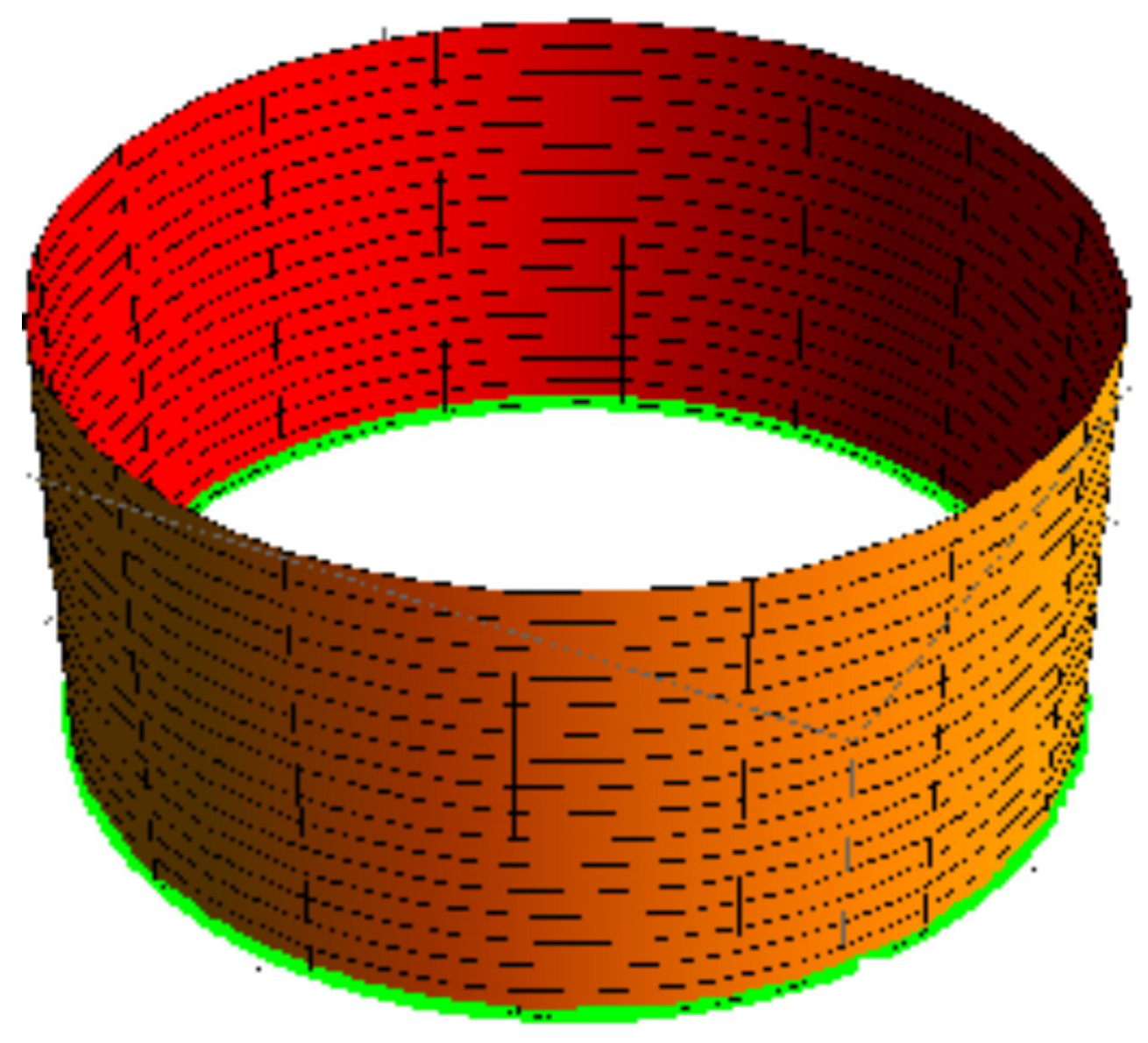
(A) By letting
, for example, the type-3 Bishop frame can be gained as
. The parametric form of the sweeping surface family can be written as
For
and
, the sweeping surface is displayed in
Figure 1. The developable surface
is a cylinder, where for
and
, the surface is shown in
Figure 2.
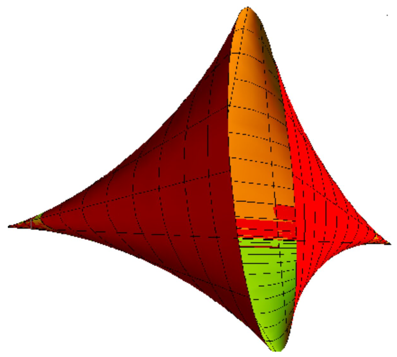
(B) For
, the type-3 Bishop frame can be obtained as
Hence, from Equations (
40) and (
41), we have
Thus, the parametric form of the sweeping surface family can be written as
For
and
, the sweeping surface is shown in
Figure 3. Furthermore, the developable surface
is a cone, where for
, the surface is shown in
Figure 4.
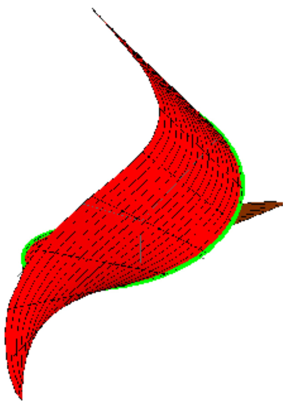
Then,
. If we choose
, for example, the type-3 Bishop frame can be expressed as
By a similar procedure as in Example (1), the sweeping surface family can be written as
Figure 5 shows the surface when
and
. Since we have
, the surface
is a tangent surface, where
and
(see
Figure 6).


