Article

Fluctuating Flexoelectric Membranes in Asymmetric Viscoelastic Media: Power Spectrum through Mechanical Network and Transfer Function Models

by
Edtson Emilio Herrera-Valencia
1 and
Alejandro D. Rey
2,*
1
Unidad de Bioingeniería, Laboratorio de Reología y Fenómenos de Transporte, L-7/PA, Unidad Multidisciplinaria de Investigación Experimental Zaragoza (UMIEZ), Carrera de Ingeniería Química, Facultad de Estudios Superiores Zaragoza, Universidad Nacional Autónoma de México, Batalla 5 de Mayo S/N, Ejército de Oriente, Ciudad de México 09230, Mexico
2
Department of Chemical Engineering, McGill University, 3610 University Street, Montréal, QC H3A2B2, Canada
*
Author to whom correspondence should be addressed.
Symmetry 2023, 15(5), 1004; https://doi.org/10.3390/sym15051004
Submission received: 10 March 2023 / Revised: 10 April 2023 / Accepted: 25 April 2023 / Published: 29 April 2023
(This article belongs to the Special Issue Structural, Optical and Hydrodynamic Properties of Liquid Crystals)

Abstract

:
Flexoelectric liquid crystalline membranes immersed in asymmetric viscoelastic media is a material system model with physiological applications such as outer hair cells (OHCs), where membrane oscillations generate bulk flow. Motivated by this physiological process, here we extend our previous work by characterizing the force transmission output of our model in addition to viscoelastic fluid flow, since solid–fluid interactions are an essential feature of confined physiological flow and flow in immersed elastic structures. In this work, the rigidity of the confinement results in a passive force reception, while more complete solid–fluid interactions will be considered in the future. A significant contribution of this work is a new asymmetry linear viscoelastic electro-rheological model and the obtained implicit relation between force transmission and flow generation and how this relation is modulated by electric field frequency and the material properties of the device. Maximal force and flow are found at resonant frequencies of asymmetry viscoelastic bulk phases, flexoelectric and dispersion mechanisms through the elastic and Womersley numbers.

Graphical Abstract

1. Introduction

Liquid crystalline organization, structure, and properties are found in a variety of biological systems, whose behavior is specified by complex processes [1,2]. The science of liquid crystal has been used in biological systems such as: (i) plants, (ii) insects, and (iii) membranes and living matter physics [3]. This paper presents a new asymmetric rheological model to describe the complex behavior of a thermodynamical system consisting of two viscoelastic liquid phases and a flexoelectric solid system, which can be applied to the modeling of the outer hair cells of mammalians [4,5,6]. It has been demonstrated that the rheology of the OHC is the key issue in the amplification of sound and its relationship with the natural electrophysiological field in the human body [4,5,6].
Mathematical theories have been used to characterize the nonlinear physics in the OHC [6]. The most remarkable physiological property in the OHC is called flexoelectricity [7,8,9]. The shape of the electrical field, material properties of the liquids, and the solid membrane are the most important issues of the power viscoelastic dissipation and their impact on the ability to tune sound information [4,5,6]. Figure 1 shows sensor (top) and actuator (bottom) modes of flexoelectricity, including energy harvesters, stress sensors, fluid pumps, and force generators; we note that the OHC, which is the topic of this paper, corresponds to the fluid pump and force generator device (bottom left in Figure 1 [9,10]).
In Table 1, we summarized directly related theoretical applications of the flexoelectric membranes, involved in the functioning of the sensor and actuator devices shown in Figure 1. Many of these devices involve dissipative bulk fluid flows (first, second rows) or membrane/filament dissipation (third–fifth rows), and the latter require new couplings between geometry and dissipation (sixth row), which is a topic of emerging research [3,4,5,9,10,11,12,13] and central to transient flexoelectric devices (seventh row).
Next, we focus on the aspects of OHCs directly related to this paper [3,4]. A number of analytical approaches have been employed to simulate the changes in the average membrane curvature of a flexoelectric membrane as a function of the electrical field [3,4] (and references therein). Rabbits et al. 2009 [14] analyzed the power efficiency of outer hair cell somatic electromotility with an electro-mechanical model based on first principles. Their results showed a frequency dependence of the power resonance, which is a function of the material parameters in the system [14]. Furthermore, some authors have employed electro-mechanical models to describe the electro-motility, and the stress of the membrane capacitance of the auditory cell in the outer hair cell has been studied at length with a mechanical viscoelastic model [15,16]. In addition, the frequency voltage and tension dependent lipid mobility in the OHC plasma membrane has been investigated using an electro-mechanical model [14,15,16,17]. Electro-motility in the cochlea system and the stereociliary columns in the mammalian cochlear hair have been studied at length using complex mathematical models [15,16,17,18,19,20]. From a mechanic-electrodynamic point of view, the mechanism effects of the electric and magnetic fields on cells have been analyzed [21]. In addition, Lahlou et al. (2023) [22] have been working on the genetics of auditory hair cells to develop new stem cell therapies. These models include the mechanical response of isolated cochlear OHCs, viscoelastic forces, start-up mechanisms, and linear viscoelasticity [23,24]. Furthermore, other researchers have developed the description of lipid mobility, plasma membrane in terms of electro-mechanical approaches, liquid crystal theories, and transport momentum and rheology constitutive equations [24,25]. A distinguishing feature of the approach is the full integration of flexoelectricity, membrane elasticity, and high-order viscoelasticity of surrounding fluids, coupling flexoelectric membrane shape equations with linear momentum equations that describe complex viscoelastic flows [3,4]. Several aspects of design/control/prediction application in the flexoelectric energy conversion device deserve discussion [9,10]. Based on our previous work [3,4,5], it has been established that the mechanical network analogy in terms of the elasticity of the flexoelectric membrane operating in parallel with viscoelastic elements provides the necessary dynamic structure to produce extrema in the viscous power spectrum of the surrounding media [3,4,9,10].
Since these viscoelastic structural elements represent the surrounding viscoelastic media and have a strong impact on power resonance, a robust, generic, and well-characterized model will be useful [26,27].
One of the main objectives of the aforementioned research is to find the flow rate and power dissipated in the surrounding viscoelastic fluids induced by the changes in the membrane curvature as a consequence of the imposed time-periodic electric field [3,4,5]. In order to include the physical nature of the contacting and surrounding fluids, several rheological constitutive equations have been employed to describe the momentum transfer [3,4,5,10], including Euler (inviscid fluid) [10], Newton [5], and variants of the Maxwell models [3,4,5]. In these previous works, the average membrane curvature vs. applied electrical was investigated [3,4,5]. Another important issue considered in the present work is to establish a wider understanding of membrane-based flexoelectric outputs and to find the relationships between the driven electrical force (input), volumetric flow, and inertial-viscoelastic wall stress (outputs) [3,4]. Figure 2 shows a schematic of a fluctuating membrane that is attached to an elastic substructure (pillars, base filaments; see ref. [12]). Hence, understanding and characterizing force transmission from the fluid flow generated by the oscillating membrane onto the elastic supporting structures are essential [26,27]. The interaction between the liquid viscoelastic phases and solid wall has been found in nonlinear biomaterials [5,26,27]. Notwithstanding, and despite all the theoretical and experimental works, there are no studies that relate the two transfer functions: (i) electric field-inertial-viscoelastic volumetric flow rate transfer function TF and (ii) electric field-inertial-viscoelastic wall stress transfer function TS, which is the main focus of this work and can be synthetized as an implicitly coupling stress-flow relation F:
T S ω Stress - Transfer - Function = F T F ω Flow - Transfer - Function
where F is an important function in flexoelectric devices, and whether it is unique or multivalued. Figure 3 succinctly summarizes the methodology we developed to find the function F (Figure 3III). We first formulate and solve the device model using a control-type transfer function formalism, indicated in Figure 3II, that can be summarized as:
O ω E ω = T X ω = Re T X ω + i Im T X ω ;   X = { F , S } , O ω = { Q ω , σ ω }
where the output vector O is given by the flow rate Q and wall stress σ, E is the oscillating electric field, and Re [Tx(ω)] is the real part and Im [Tx(ω)] the imaginary part of the quantity in question [3,4]. The transfer functions will have in-phase (real) and out-of-phase (imaginary) components with respect to the input electric field. In principle, the result of the control-type transfer function (Figure 3II) is sufficient to determine F (Figure 3III). Given the complexity of the material information (viscoelasticity, membrane elasticity, etc.), an organizing design principle is needed, and here we use the analogue mechanical network model (Figure 3I). The mechanical network guides the selection and arrangement (in series, in parallel) of the elastic and viscous mechanical elements. Feeding this design information (Figure 3I) in conjunction with the control analysis (Figure 3II) yields the sought-after relations between viscoelastic flows Q and wall stress transfer σ (Figure 3III).
Based on the facts and observations presented above, the specific objectives of this paper are:
(1)
To deduce a new general asymmetric electro rheological model for a flexoelectric membrane attached to a circular capillary tube that contains Maxwell’s viscoelastic fluids and is subjected to a fluctuating small amplitude electric field of arbitrary frequency;
(2)
To compute the flow and stress complex transfer functions vs. frequency as a function of the applied frequency and the material properties of the thermodynamic system;
(3)
To use the modeling results to characterize the complex loops of the flow and stress transfer functions;
(4)
To identify the numerical values of the dimensionless groups that lead to electromechanical force-flow conversion of potential interest to the functioning biological systems.
The outline of this paper is as follows (Figure 4).

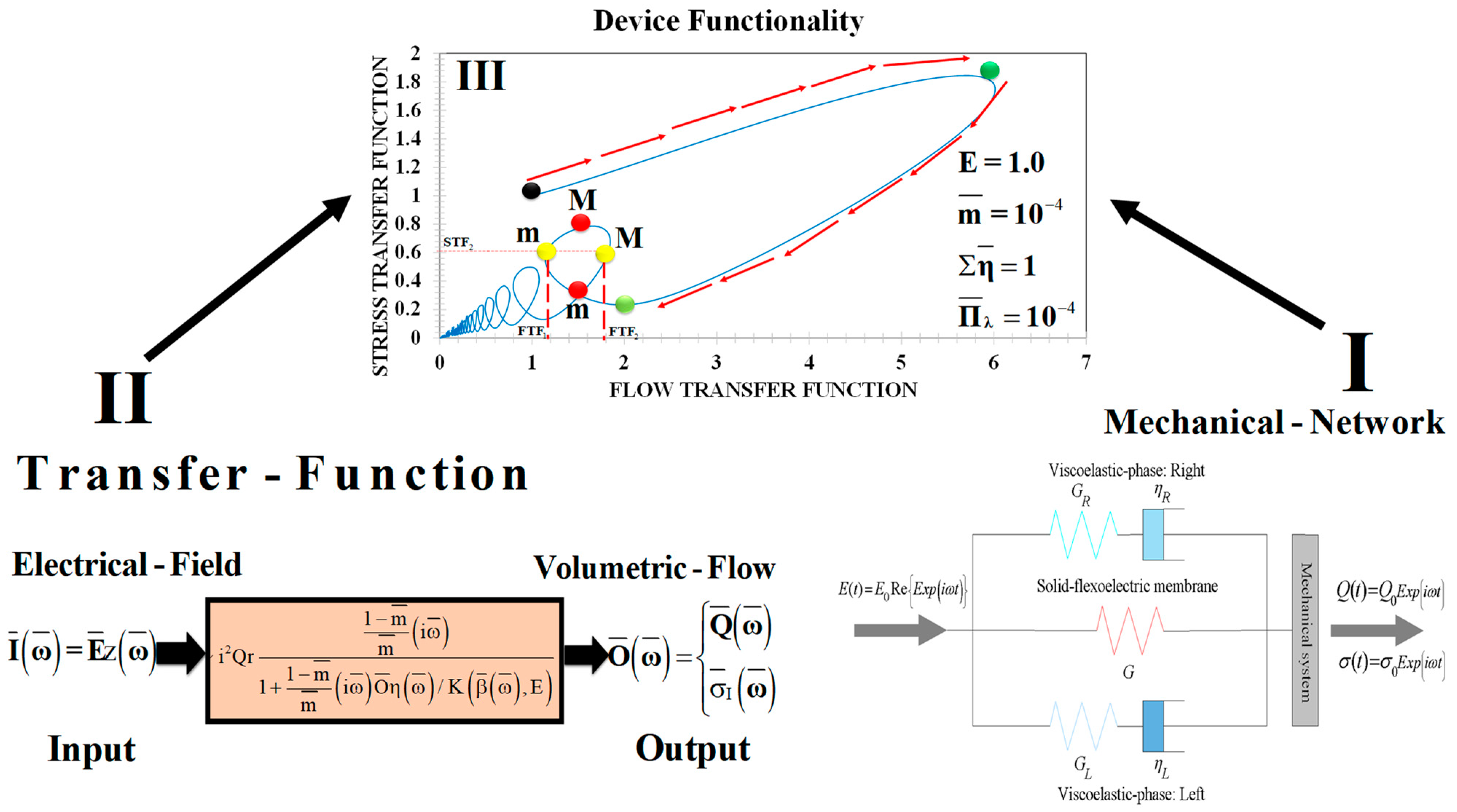
2. Mechanical Network Model

In this section, we first present the physical system for Maxwell bulk fluids that are in contact with the flexoelectric membrane and then use the mechanical spring-dashpot network model to derive the total stress tensor σ of the device as it creates a flow rate Q in the fluid phases and forces through the wall shear stress [3,4,5]. We note that the flexoelectric membrane is attached to a cylindrical tube, and the bulk fluid flow imposes a wall shear stress on the tube walls.

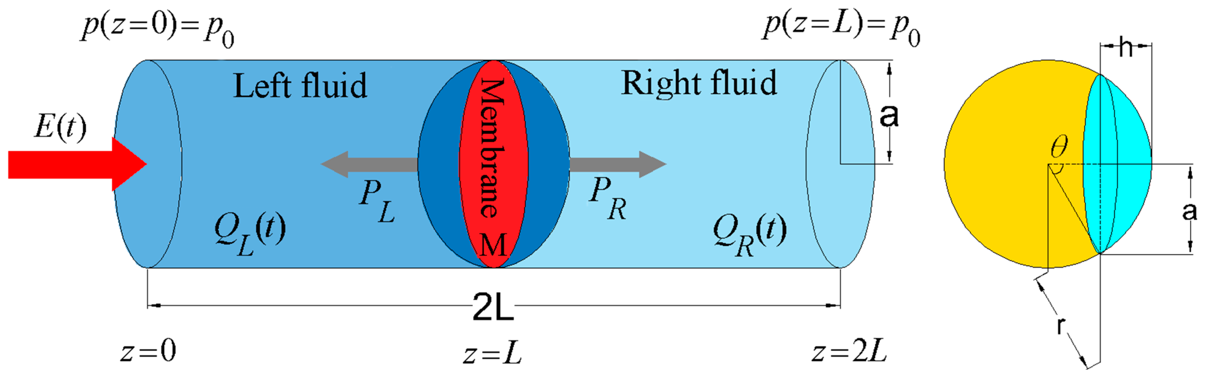
2.1. Device Material Structure and Geometry

The device considered in this paper is shown in Figure 5, since gravity plays no role, due to the overall orientation of the device. A flexoelectric membrane (red sector, M) is tethered to a cylindrical capillary system {r = a, z = L}. At the left and right sectors of the membrane, there are two Maxwell viscoelastic liquids [3,4,5,28].
The material parameters that define the device’s viscoelasticity are: (a) viscosities {ηb, ηt}, (b) relaxation times {λb, λt}, and (c) elastic flexoelectric membrane {G}, respectively [3,4,5,28]. The flexoelectric effect of the membrane caused by the imposed sinusoidal Ez(t) field and that there is not an externally imposed pressure gradient in the axial direction [3,4,5].

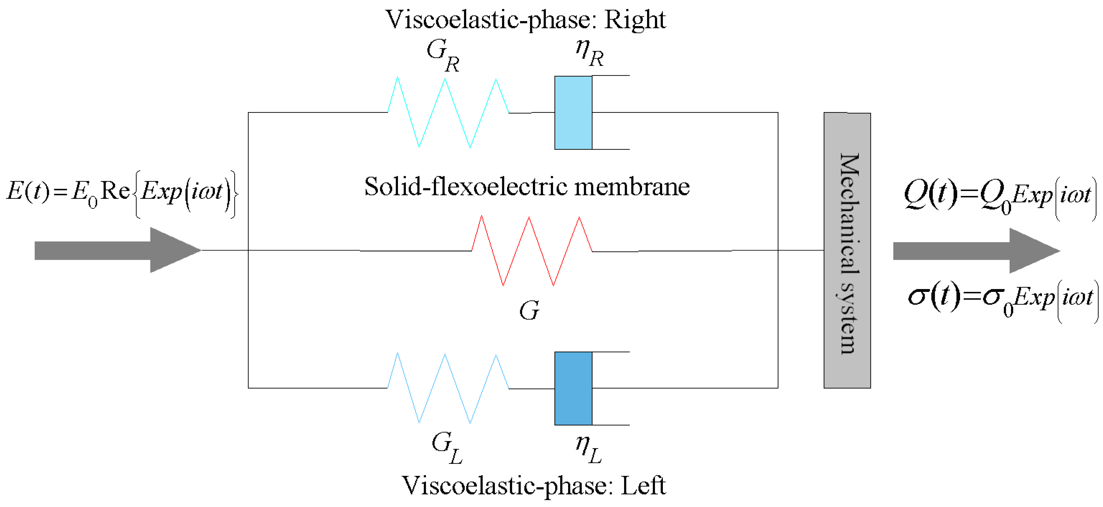
2.2. Mechanical Analogue

The mechanical analogue of the flow and force generator device (see Figure 5) is shown in Figure 6. The viscoelastic fluid elements are in parallel to the elastic flexoelectric membrane of modulus G. The selection of an in-parallel network is a key ingredient in the device model and defines the couplings between fluid flows and elastic membrane and can be easily generalized in future work to other fluids and to other elastic elements besides the membrane G.
The viscoelastic liquid phases are characterized by Maxwell linear operators. In the viscoelastic phase (Figure 5, right), the total deformation is given by γ = (γv)R + (γe)L, and the shear stress in the viscous and elastic contribution satisfies σv = σe = σR [28]. Then, taking the time derivative of the deformation dγ/dt = d(γv)R /dt + d(γe)L/dt and assuming that the viscous and elastic contribution in the system can be modeled as Newtonian fluid and Hooke solid, respectively, the following expression is obtained [28]:
2 D = γ · = 1 η R σ R + 1 G R σ R t
Using the inverse operator formalism with Dt = ∂/∂t, we get [3,4]:
σ R = η R 1 1 + λ R D t 2 D
where λR = ηR/GR, GR, and ηR are the relaxation time, elastic modulus, and viscosity of the Maxwell constitutive equation corresponding to the viscoelastic phase (Figure 5, right). Likewise, the left-side phase in Figure 5 is described by [3,4,28]:
2 D = γ · = 1 η L σ L + 1 G L σ L t
and
σ L = η L 1 1 + λ L D t 2 D
where λL, GL, and ηL are the relaxation time, elastic module, and viscosity of the left phase in Figure 5. The elasticity of the flexoelectric membrane is given by a Hooke solid equation [28]:
σ M = G γ
where G can be expressed in the following form [3,4]:
G = 2 γ 0 + 2 k 0 + k 1 4 L
and γ is the second-order strain tensor [3,4,5,11]. In Equation (6), γ0 is the interfacial surface tension at zero electric field, k0 and k1 are the membrane bending rigidity and torsion elastic moduli, and L is the characteristic axial length of the device [5,11] (See Appendix C for details of the shape membrane equation). The total stress σ of mechanical network is given by the sum of the three stress contributions [3,4]:
σ = σ L + σ M + σ R
In Equation (7), all the deformations in the elements are equal: γv = γR = γM and:
σ = η L 1 1 + λ L D t 2 D + G γ + η R 1 1 + λ R D t 2 D
and taking the time derivative
σ t = η L 1 1 + λ L D t 2 t D + G 2 D + η R 1 1 + λ R D t 2 t D
Using the reciprocal of the inverse operator, Equation (9) gives a new asymmetric cubic stress-quadratic deformation rate evolution model:
σ t + Σ λ 2 σ t 2 + Π λ 3 σ t 3 = 2 G D + Σ λ + Σ η G D t + Π λ 1 + Σ G G 2 D t 2
The fluidity operator version for Equation (10) is:
2 D = O Φ D t σ ; O Φ D t = 1 O η D t ; D t = t
where OΦ(Dt) = 1/Oη(Dt) is the fluidity operator (inverse of the complex viscosity Oη) of the Maxwell fluids and the solid flexoelectric membrane [3,4]. Note that the system describes a discontinuity due to the solid flexoelectric membrane, so we assume that the width of the flexoelectric membrane is small, and the asymmetric fluidity operator:
O Φ D t = 1 O η D t = D t G D t = D t G 1 + Σ λ D t + Π λ D t 2 1 + Σ λ + Σ η G D t + Π λ 1 + Σ G G D t 2
where the following material properties are defined [3,4]:
Σ λ = λ R + λ L ;   Π λ = λ R λ L ;   Σ G = G R + G L ;   Σ η = η R + η L
Here, ΣG = GR + GL is the total bulk elasticity, Σλ = λR + λL the total viscoelasticity, Π = λRλL the memory product, and Ση = ηR + ηL the total bulk viscosity [3,4]. In Equation (12), the fluidity operator OΦ(Dt) provides the link between stress σ and deformation rate D. Equation (10) is a variant of a Maxwell model, which describes a thermodynamic system associated with two viscoelastic liquid phases and a solid flexoelectric membrane and describes creep and stress relaxation mechanisms [3,4]. Equation (12) depends on the time differential operator Dt~1/t, which scales with the inverse of time. Note that a key point in the new developed rheological model is the asymmetry in the time derivatives of the shear stress and shear strain tensors.
The first one is of the third order, whereas the second one is of order two. This controls the mathematical shape of the resonance spectrum. Under periodic forcing of frequency ω, Dt = ω and Equation (12) admits two asymptotic limits: (i) the flexo-viscous terminal (ω → 0) mode and (ii) flexo-bulk elastic large (ω → ∞) frequency mode:
( i )   Flexo - viscous   mode : Im lim ω 0 O η   G ω , Re lim ω 0 O η   η R + η L ; ( ii )   Flexo - bulk - elastic   mode : Im lim ω O η   G +   G R + G L ω , Re lim ω 0 O η   0
where Im denotes imaginary and Re denotes real. Under small frequency, Equation (14) and Figure 6 indicate that bulk elasticity plays no role because the slow deformation rate activates only the bulk viscous dashpots; the frequency scaling in this regime is 1/ω. Under large frequency, Equation (14) and Figure 6 indicate that bulk viscosities of the two dashpots plays no role because the fast deformation rate activates only the bulk elastic springs while the dashpots are frozen. Then, we conclude that full viscoelasticity is only observed under intermediate frequencies, as discussed in full detail below. In partial summary, the network model offers an efficient route to derive the total stress tensor σ and the complex fluidity and viscosity operators {OΦ(ω), Oη(ω)} of the device [3,4]. Viscoelastic flow Q and wall stress σw can be generated at intermediate frequencies ω. These results will be used to find the norm of the complex flow and stress transfer functions in the device. These new results provide symmetric and asymmetric operators and their proper mechanical configuration.

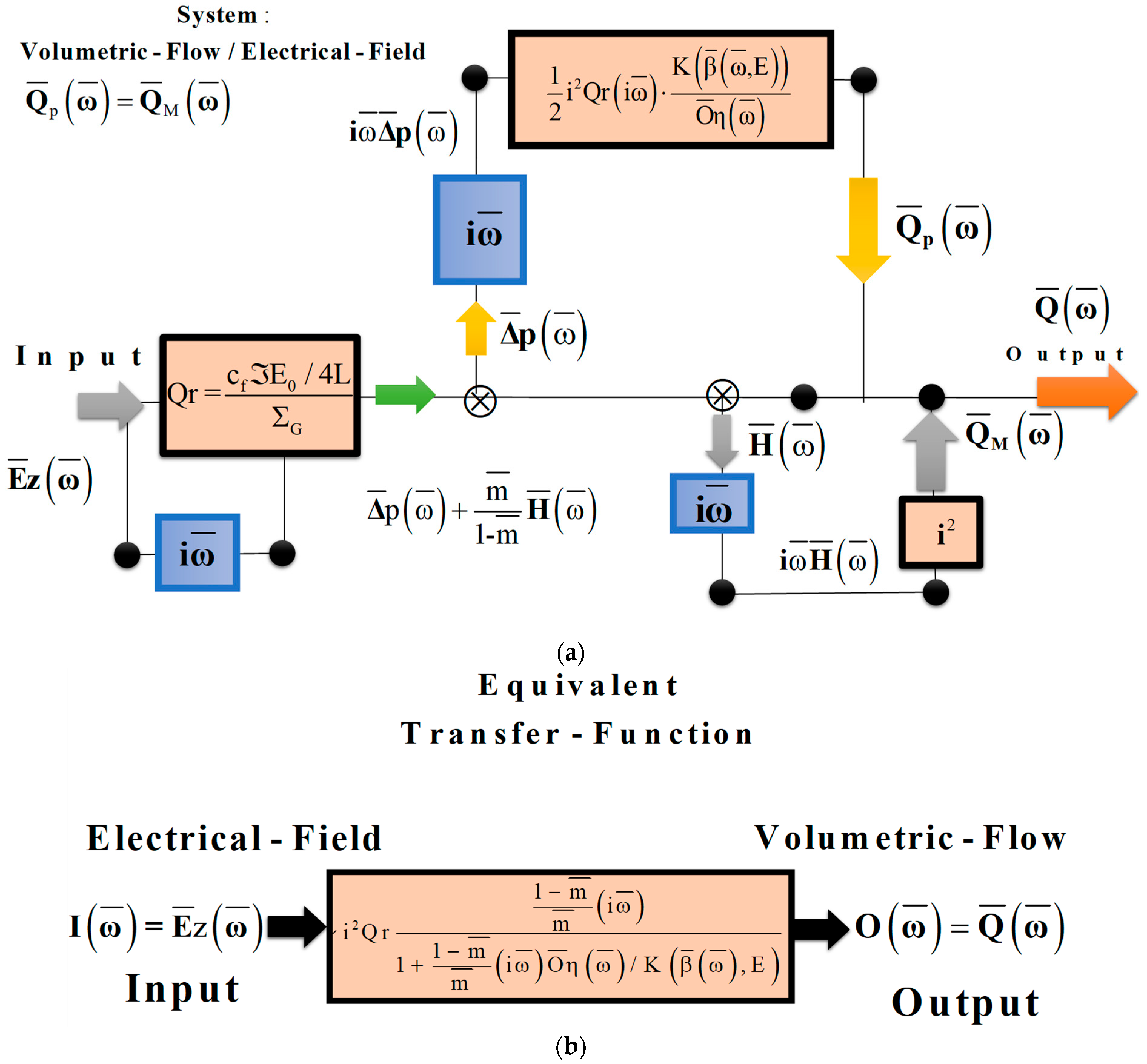
3. Transfer Functions from the Fourier Domain

In this section, we derive the transfer function using the following sequential steps: (i) using the linear momentum balance equation, we first find the axial velocity V; (ii) integrating the axial velocity, we find the volumetric flow rate Q; and, finally, (iii) identifying the device’s inputs and outputs in the Fourier domain, we find the flow FTF and stress transfer functions STF.

3.1. Continuity and Transport Momentum Equations

The mass balance equation (without chemical reaction):
ρ x t + ρ x V = 0 ;   x = { L , R }
The general Cauchy linear momentum balance equation is:
t ρ x V = T ;   x = L , R
where T includes the scalar pressure p and the unit tensor I, ρx is the density of the liquid phases, VV is the dyadic product tensor of the velocity vector field V and
T = p X I + ρ X V V σ = c f L Φ E I + ρ X V V σ
In Equation (17), cf is the flexoelectric constant ([=] Newtons/Coulomb), ℑ is the shape factor for the hemispheric cup ℑ = 8/a2, L is the characteristic axial length, and ΦE is the electrical potential field [3,4,5,11].

3.2. Complex Axial Velocity and Boundary Conditions

Assuming incompressibility in the liquid viscoelastic phases, isothermal process, the gravitational forces are neglected, the velocity vector field V has only one component different from zero, i.e., V × ez = (0, 0, Vz(r, t)), and the process depends on time [3,5]. The fluid is sheared by the effect of the applied electric field, and once the Equations (16) and (17) are combined, the following expression is obtained for the velocity field:
V r , t = c f / L O Φ D t 2 + i 2 O Φ D t Σ ρ D t Φ E t
In Equation (18), OΦ(Dt) is the linear operator defined in Equations (12) and (13), Σρ = ρR + ρL and Dt = ∂/∂t is the time partial derivative of the rheological equation of state [3,4]. The linear partial differential model given by Equation (18) satisfies the following boundary conditions: (i) non-slip mechanisms at the wall, and (ii) the symmetry of the velocity field [3,4]:
V z r = a , t = V r , t e z r = a = 0
V z r r = 0 = r V r , t e z r = 0 = 0

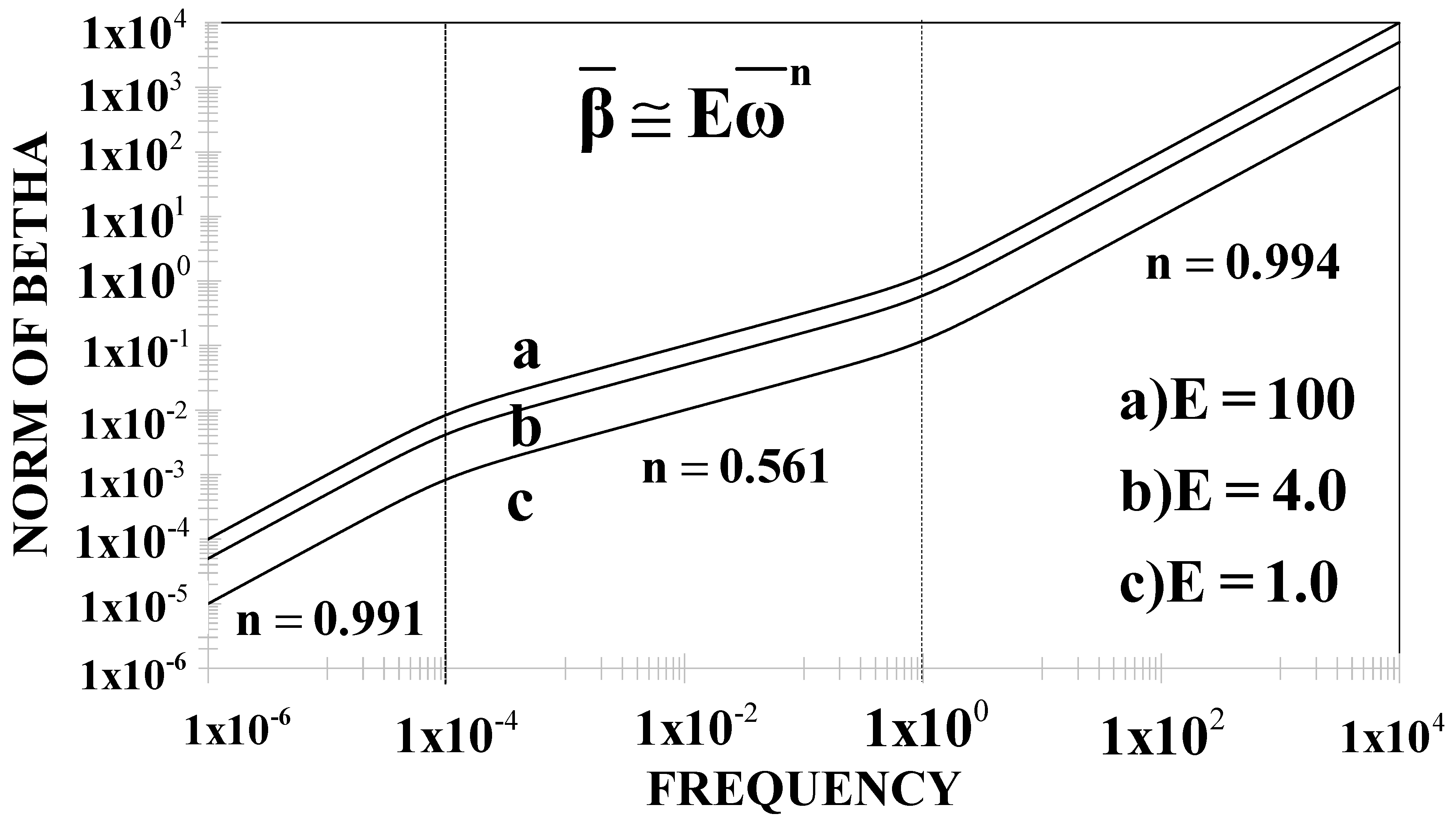
3.3. Formulation in the Fourier Domain and Complex Wave Vector β(ω)

Multiplying Equation (18) for the axial unit vector ez and applying the standard Fourier transform
F ω = 1 2 π f t e i ω t d t
the axial velocity Vz (r,ω) in the Fourier domain is obtained:
V z r , ω = c f / L O Φ i ω 1 r r r r + β 2 ω z Φ E ω
In Equation (22), the key reciprocal length scale parameter β (ω) appearing in the denominator of Equation (22) is given by:
β ω = Re β ω + I Im β ω = i 3 / 2 Σ ρ ω O Φ i ω
The parameter β(ω) is defined as the complex wave vector associated with the axial velocity Vz (ω), which is the inverse of a characteristic length [3,4]:

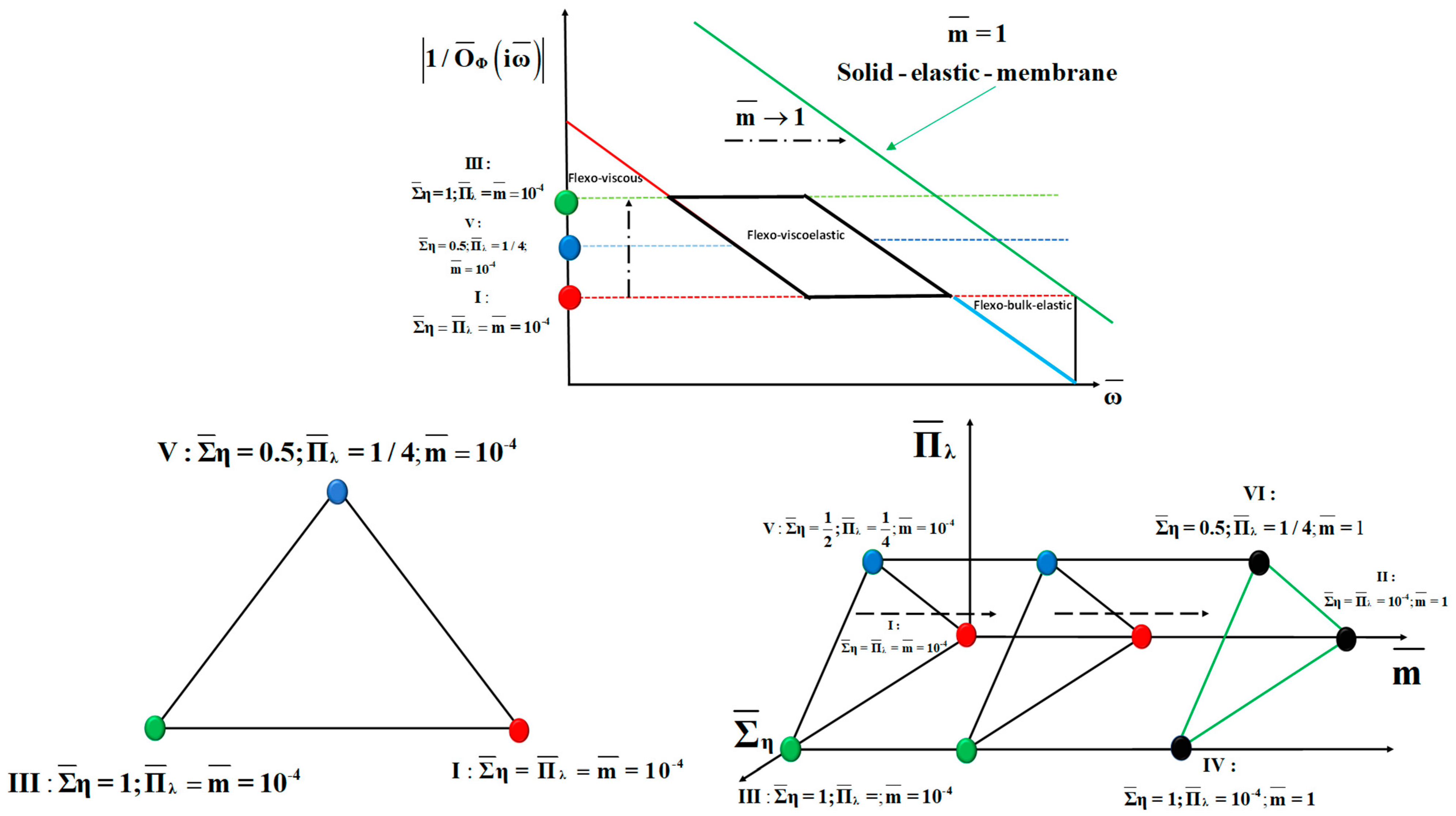
3.4. Scales, Dimensionless Numbers, and Device Mode Classification Based on Kinematics and Rheology

In this section, we discuss (i) the length and time scales and dimensionless numbers of this device and (ii) use them to present a device mode classification in terms of flexo-viscous-bulk elastic contributions.
(a)
Scales and dimensionless numbers
Equations (12) and (23) provide a basis to characterize the device modes according to frequency and dimensionless numbers; quantities with overbars are dimensionless (See Appendix A). In order to simplify the analysis of the physical system, we propose scaling laws to simplify the physical interpretation and to find the dimensionless groups needed to identify the macroscopical forces in the system. The details of the dimensionless variables and groups is explained in Appendix B. In what follows, all the variables are in dimensionless form.
The wave vector β ¯ ω ¯ in Equation (23) is a crucial parameter and has units of the inverse of a characteristic length and depends on imposed frequency, the dimensionless number E (defined below), and the rheology and flow through the fluidity operator O ¯ Φ i ω ¯ .
β ¯ ω ¯ = Re β ¯ ω ¯ + I Im β ¯ ω ¯ = i 3 / 2 E 1 / 2 ω ¯ O ¯ Φ i ω ¯
Equation (24) shows that the complex wave vector β ¯ ω ¯ depends on the product of the frequency ω ¯ ; the fluidity operator O ¯ Φ i ω ¯ can be expressed as follows:
O ¯ Φ i ω ¯ = 1 O ¯ η i ω ¯ = i ω ¯ 1 m ¯ m ¯ 1 + i ω ¯ + Π ¯ λ i ω ¯ 2 1 + 1 + 1 m ¯ m ¯ Σ ¯ η i ω ¯ + Π ¯ λ m ¯ i ω ¯ 2
In the fluidity operator Equation (25), there are three fundamental dimensionless groups: (i) total bulk viscosity ( Σ ¯ η ), (ii) memory ( Π ¯ λ ), and (iii) elastic membrane ratio ( m ¯ ). In Equation (24), the complex wave vector β ¯ ω ¯ can be expressed in terms of the complex compliance J ¯ * ω ¯ , since we are interested in analyzing the start-up mechanisms in the system [28] (inertial mechanisms).
β ¯ ω ¯ = i 2 E 1 / 2 ω ¯ J ¯ * ω ¯
In Equation (26), the complex compliance J*(ω) is given by:
J ¯ * ω ¯ = 1 G ¯ * ω ¯ = O ¯ Φ i ω ¯ i ω ¯
The dimensionless elastic number E (Equation (26)) is the ratio of two fundamental numbers: (i) the Weissenberg (We) and (ii) the Reynolds number (Re) [28]. The elastic number E is given by [29,30,31]:
E = W e Re = Σ λ Σ ρ a 2 / Σ η
Note that there is no imposed macroscopic velocity in the system, and for this reason it is better to explain all the mechanisms in terms of the elastic number E, instead of other dimensionless numbers such as (i) Deborah, (ii) Mach, (iii) Newtonian Womersley number, and (iv) vibratile Reynolds [32,33]. The wavelength vector b (Equation (26)) deals with the pulsating Womersley number related to the competition between the viscous and oscillatory mechanisms [32,33]:
W 0 2 = a 2 Σ ρ Σ η ω = t v ω
where tv is visco-inertial time scale. In terms of the elastic number E, the non-Newtonian Womersley number (Wo) is given by [34,35,36,37]:
W 0 = t v t v e t v e ω = 1 t v e / t v t v e ω = E 1 / 2 ω ¯
where time scale tve can be read off [34,35,36,37]. Note that Wo and E numbers are related through the inverse relation in Equation (28). The Womersley number describes the competition between the flow frequency and the dissipation associated with the viscous (Newtonian) or viscoelastic (non-Newtonian) effects, and it increases with frequency [34,35,36,37,38].
(b)
Device mode classification based on flow kinematics
Equation (23) indicates the crucial importance of the complex velocity wave vector β ¯ ω ¯ ; units of beta: 1/length. Hence, we expect that this reciprocal length scale provides a direct link to the classification of the modes presents in the device as the frequency increases. The computed norm of the complex wave vector as a function of dimensionless frequency is shown in Figure 7. It clearly shows the three-mode response: flexo-viscous with linear frequency scaling, intermediate flexo-viscoelastic with square-root frequency scaling, and flexo-bulk elastic linear scaling [29,30]. The role of the elastic number is a vertical shift [31,32]. This primitive quantity β ¯ ω ¯ associated with the velocity field shows the scaling of its norm with the Womersley (Wo) [33,34,35,36,37,38] and elastic (E) number [31,32] is:
( i )   f l e x o v i s c o u s : β E ω ¯ = E 2 W 0 2 = W e / Re 2 W 0 2 ( i i )   f l e x o v i s c o e l a s t i c : β E ω ¯ = E W 0 = W e / Re W 0 ( i i i )   f l e x o b u l k e l a s t i c : β E ω ¯ = W e / Re 2 W 0 2
(c)
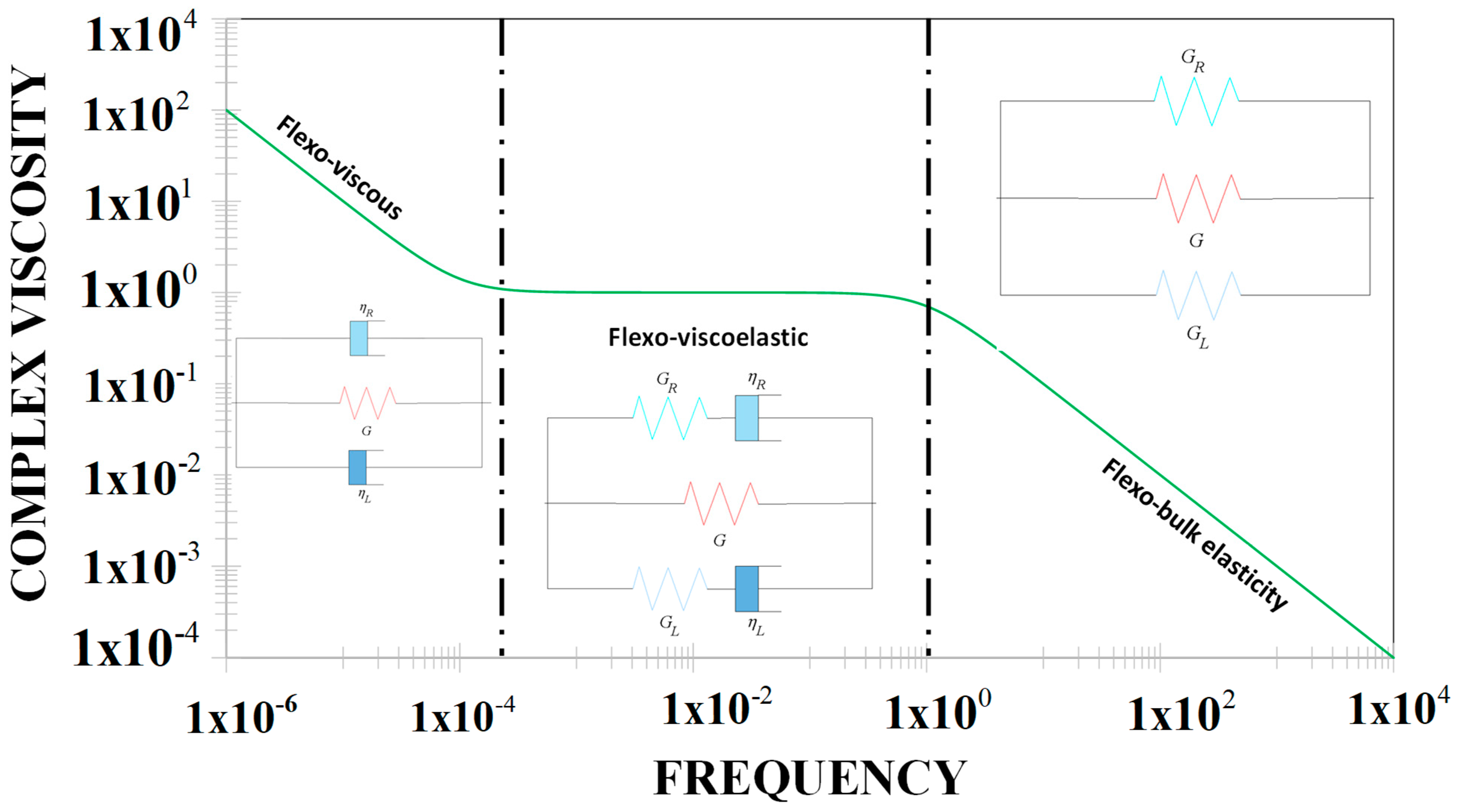
Device mode classification based on rheology
A complementary device mode classification can be conducted based on the complex viscosity function O ¯ η (see Equation (11)). In Figure 7, complex viscosity is plotted vs. frequency for our visco-elastic rheological model. Herrera-Valencia and Rey (2018) showed that these dimensionless numbers describe a 3D-prismatic space [3]. They established that the system optimum conditions are a floppy membrane ( m ¯ = 1 × 10 4 ), total bulk viscosity (large dissipation, Σ ¯ η = 1 ), viscoelastic contrast between the bulk fluids ( Π ¯ λ = 1 × 10 4 ), and balanced flexoelectric and bulk elastic mechanisms (Qr = 1), defined in Equation (34) below [3].
Figure 8 shows the three modes envisioned by analyzing the dashpot-spring network mentioned above:
( i )   Flexo - viscous   mode : Im lim ω 0 O ¯ η   G ¯ ω ¯ = G ¯ W 0 2 E , Re lim ω 0 O ¯ η   Σ ¯ η = c o n s t a n t ( ii )   Flexo - viscou - elastic   mode : O ¯ η = c o n s t a n t ( iii )   Flexo - bulk - elastic   mode : lim ω O η   G ¯ + Σ ¯ G ¯ ω ¯ = G ¯ + Σ ¯ G ¯ W 0 2 E
Hence, the rheological characterization clearly distinguishes the three modes; more importantly, it shows the band of frequencies where we can expect resonances and hence more flow and more shear wall stress.
Below, we will discuss how the complex viscosity-frequency responds to changes in material properties, in particular at intermediate frequencies.

3.5. Complex Axial Velocity

The solution of Equation (18) is given in terms of a combination of zero order Bessel functions:
V ¯ z r ¯ , ω ¯ = C ¯ 1 J 0 β ¯ ω ¯ r ¯ + C ¯ 2 Y 0 β ¯ ω ¯ r ¯ + Q r O ¯ Φ i ω ¯ β ¯ ω ¯ 2 ¯ z Φ ¯ E ω ¯
where Qr is the ratio between the flexoelectric and bulk elastic mechanisms, and it is given by:
Q r = a c f E 0 / L Σ G = F l e x o E l e c t r i c M e c h a n i m s B u l k E l a s t i c M e c h a n i m s
In Equation (33), {J0, Y0} are the classical special Bessel functions [3]. From the boundary conditions (Equations (19) and (20)), the constants C ¯ 1 ω ¯ and C ¯ 2 ω ¯ are calculated as follows:
C ¯ 1 ω ¯ = Q r 1 J 0 β ¯ ω ¯ O ¯ Φ i ω ¯ β ¯ 2 ω ¯ i 2 ¯ z Φ ¯ E ω ¯
C 2 ω ¯ = 0
The constant C ¯ 2 ω ¯ must be set up to zero because, physically, the velocity cannot be infinity at r ¯ = 0 . Then, the general profile for the axial velocity V ¯ z r ¯ , ω ¯ is:
V ¯ z r ¯ , ω ¯ = Re V ¯ z r ¯ , ω ¯ + i Im V ¯ z r ¯ , ω ¯ = Q r O ¯ Φ i ω ¯ β ¯ ω ¯ 2 J 0 β ¯ ω ¯ J 0 β ¯ ω ¯ r ¯ J 0 β ¯ ω ¯ ¯ z Φ ¯ E ω ¯
Equation (37) is the sum of an r-dependent function and an r-independent driving force term that always vanishes at the bounding walls. The effectiveness of the driving term is regulated by the flexoelectricity number Qr, and it is zero for a purely elastic membrane. The norm of the complex velocity is:
V ¯ z r ¯ , ω ¯ = Re V ¯ z r ¯ , ω ¯ 2 + Im V ¯ z r ¯ , ω ¯ 2
The velocity at the center of the cylindrical geometry is:
V ¯ max ω ¯ = V ¯ z r ¯ = 0 , ω ¯ = Q r O ¯ Φ i ω ¯ β ¯ ω ¯ 2 J 0 β ¯ ω ¯ 1 J 0 β ¯ ω ¯ ¯ z Φ ¯ E ω ¯

3.6. Complex Volumetric Flow Rate and Transfer Functions

The right and left volumetric flow rates Q ¯ R ω ¯ and Q ¯ L ω ¯ (see Figure 5) are induced by the speed of the flexoelectric membrane as it curves into the contacting viscoelastic liquid phases:
Q ¯ ω ¯ = Q ¯ R ω ¯ = Q ¯ L ω ¯ = 2 0 1 V ¯ z r ¯ , ω ¯ r ¯ d r ¯
Replacing the axial velocity profile (Equation (37)) into the volumetric flow rate (Equation (40))
Q ¯ ω ¯ = Q r O ¯ Φ i ω ¯ β ¯ ω ¯ 2 1 2 J 1 β ¯ ω ¯ / β ¯ ω ¯ J 0 β ¯ ω ¯ ¯ z Φ ¯ E ω ¯
Equation (41) can be rewritten in the following compact form:
Q ¯ ω ¯ F l o w   r a t e = T ¯ F ω ¯ F l o w   transfer   function σ ¯ F E F l e x o e l e c t r i c   s t R e s s
In Equation (42), T ¯ F ω ¯ , σ ¯ F E are the complex flow transfer function and the wall flexoelectric stress force in the system (See Appendix C). The wall flexoelectric stress force σ ¯ F E is given in terms of the negative of the electrical potential:
σ ¯ F E ω ¯ = 1 2 E ¯ z ω ¯ = 1 2 ¯ z Φ ¯ E ω ¯

3.7. Flow Transfer Function ( T ¯ F ω ¯ )

Starting from Equations (41) and (42), the dimensionless complex flow transfer function, T ¯ F ω ¯ can be expressed as follows:
T ¯ F ω ¯ = Q r F l e x o E l e c t r i c E l a s t i c O ¯ Φ i ω ¯ R h e o l o g y F ¯ β ¯ D i s p e r s i o n
where the nonlinear dispersion contribution F ¯ β ¯ is given by:
F ¯ β ¯ = 8 i 2 β ¯ 2 ω ¯ 1 2 J 1 β ¯ ω ¯ / β ¯ ω ¯ J 0 β ¯ ω ¯
It is important to note that the dispersion mechanisms depend only on the wave vector β ¯ ω ¯ parameter, through the elastic E number, the rheology (fluidity operator), and the frequency. Mathematically, the norm of the flow transfer function (Equation (44)) is given by:
T ¯ F ω ¯ , m ¯ , Π ¯ λ , Σ ¯ η , E = Re [ T ¯ F ω ¯ , m ¯ , Π ¯ λ , Σ ¯ η , E ] 2 + Im [ T ¯ F ω ¯ , m ¯ , Π ¯ λ , Σ ¯ η , E ] 2

3.8. Stress Transfer Function (Ts)

In this section, the dimensionless stress transfer function T ¯ S ω ¯ is derived. The wall flexoelectric stress (mentioned above) is:
σ ¯ F E ω ¯ = 1 2 E ¯ z ω ¯
The wall stress σ(ω) can be estimated in a straightforward calculation using Equations (11) and (12):
σ ¯ ω ¯ = 1 O ¯ Φ i ω ¯ V ¯ z ω ¯ r ¯ r ¯ = 1 = 1 O ¯ Φ i ω ¯ C ¯ 1 ω ¯ β ¯ ω ¯ J 1 β ¯ ω ¯
Once the constant C ¯ 1 ω ¯ (Equation (31)) is inserted into Equation (41), the dimensionless stress transfer function T ¯ s ω ¯ (STF) is obtained:
σ ¯ ω ¯ Inertial - s t r e s s = T ¯ S β ¯ ω ¯ S t r e s s   T r a n s f e r   F u n c t i o n σ ¯ FE ω ¯ F l e x o E l e c t r i c   S t r e s s
The dimensionless stress transfer function T ¯ s ω ¯
T ¯ S β ¯ ω ¯ = 2 Q r J 1 β ¯ ω ¯ / β ¯ ω ¯ J 0 β ¯ ω ¯
The norm of the complex stress transfer function is given by:
T ¯ S ω ¯ , m ¯ , Π ¯ λ , Σ ¯ η , E = Re [ T ¯ S ω ¯ , m ¯ , Π ¯ λ , Σ ¯ η , E ] 2 + Im [ T ¯ S ω ¯ , m ¯ , Π ¯ λ , Σ ¯ η , E ] 2
When increasing the frequency, beta β ¯ ω = i 3 / 2 E 1 / 2 ω ¯ O ¯ Φ i ω ¯ samples the zeroes of the oscillatory Bessel function, indicating oscillations in the flow and force transfer functions. The main equations characterize this device and the three-mode characterization using kinematics and rheology. The first important equation is the complex flow transfer function (FTF, Equations (44)–(46)), which gives us the relation between the input (Ez) and the output (Q). The second important equation is the stress transfer function (STF, Equations (49)–(51)). This equation deals with the electrical wall stress (input) and the inertial-electrical wall stress (output). These results are essential to compute the resonance curves and the stress-flow loops of the electro-mechanical device (Real and Imaginary flow-stress loops are explained in detail in Appendix D).

4. Device Functionality: Flow and Force Generation

The purpose of the device studied in this paper is to create volumetric flow and to generate wall forces, and we find that an implicit relation between the two characteristic transfer functions (flow T ¯ F ω ¯ and force T ¯ s ω ¯ ) best characterizes the device functionality. Thus, the connection between the FTF and STF T ¯ F ω ¯ , T ¯ s ω ¯ , as a function of the flexo-elastic-bulk viscoelastic mechanisms, needs to be understood and characterized. Without ambiguity, we do not discuss here real and imaginary components as that is done in the next numerical section (See Appendix E for 3D parametric classification of the mean dimensionless macroscopical groups). The relation between the two complex transfer functions is repeated here for clarity and continuity; it is given by:
T ¯ S ω ¯ = F T ¯ F ω ¯
Using Equations (44), (45) and (50), the device functionality is given by:
T ¯ S β ¯ ω ¯ = Q r + β ¯ 2 ω ¯ 8 O ¯ Φ i ω ¯ T ¯ F i ω ¯
Using the definition of wave vector β ¯ ω ¯ (Equation (24)), the following equivalent form is obtained:
T ¯ S β ¯ ω ¯ = Q r + i 2 E 1 i ω ¯ 8 T ¯ F i ω ¯
At small and large frequencies, Equation (54) reflects the expected solid modes:
f l e x o v i s c o u s   m o d e : lim ω ¯ 0 T ¯ S β ¯ ω ¯ = Q r lim ω ¯ 0 T ¯ F β ¯ ω ¯ = 0 f l e x o b u l k e l a s t i c   m o d e : lim ω ¯ T ¯ S ω ¯ = 0 lim ω ¯ T ¯ F ω ¯ 8 Q r O ¯ Φ i ω ¯ β ¯ 2 ω ¯

5. Computational Results

Next, we present a systematic study as follows: (a) use Equation (45) to find the flow transfer function FTF, and (b) use Equation (50) to determine the stress transfer function STF. The main dimensionless numbers are: (i) total bulk viscosity, (ii) memory, (iii) elastic ratio, and (iv) elastic number E. The final output of this analysis provides (a) flow and stress transfer functions, (b) device functionality (Equation (53)), (c) material properties, and (d) electric field frequencies (ω) that simultaneously optimize (i.e., achieve high values) flow and force generation.

5.1. Elastic Number E

In Figure 9a,b, the norm of FTF and STF vs. frequency is analyzed for the decreasing E number. Except for Figure 10a, in all the simulations the value of the dimensionless groups, the representative dimensionless material parameters employed in the simulations, are: (i) m ¯ = 1 × 10 4 , (ii) Σ ¯ η = 1 (iii) Π ¯ λ = 1 × 10 4 and Qr = 1.
It is important to note that both transfer functions display primary and secondary resonances. The figures shows: (a) at low frequencies, the norm of the FTF and STF are constant and independent of the frequency, (b) the dominant frequency occurs at the first primary peak and is much larger than the other secondary resonance peaks, (c) the flow transfer function has a train of secondary peaks whose amplitude gradually decrease, (d) for the dimensionless numbers chosen, the value of the resonance frequency is close to ω ¯ 20 , and (e) the resonance of the flow transfer function is larger than for the stress transfer function system. We note that the norm of FTF shows similar resonance behavior as other bio-physic systems (occlusion in human blood arteries) [4,5,6,7,8].

5.2. Membrane Elasticity

In Figure 10a, the norm of the FTF as a function of frequency is analyzed in terms of the elastic ratio m: m ¯ = a : 1 × 10 4 , b : 1 × 10 1 ; c : 5 × 10 1 . The behavior is analogous to that shown in Figure 9. The net effect of increasing the elastic ratio is to decrease the resonance peak in both transfer functions; to avoid redundancy, we only show the FTF.

5.3. Velocity Profile

In Figure 10b, the norm of the complex velocity vs. radial coordinate is shown for representative material conditions. The dimensionless numbers used in the simulations are the same as Figure 8 and Figure 9a. Panel A shows the effect of the frequency over the norm of the velocity profile. It is clear that for some particular frequencies, the system displays oscillatory behavior instead of the classical velocity profile. Panels B–D show the effect of the elastic number E, which is related to the viscoelastic and inertial mechanisms. Notice that when the inertia mechanisms are small, it displays a symmetric velocity profile, whereas the opposite effect is clearly seen when the inertia mechanisms are dominant over the viscous and viscoelastic forces. Finally, the oscillatory behavior is a coupled mechanism between frequency, viscous, and viscoelastic behavior through a critical E number.
Again, in these velocity profiles we see that increasing E = We/Re dampens oscillations, consistent with previous observations. The oscillations shown in Figure 10b come from the contribution of the resonance and anti-resonance of the transfer function. The numbers of them, deals are controlled for all the mechanisms in the system (bulk-viscous, viscoelastic, bulk-elastic, flexoelectric, etc.).

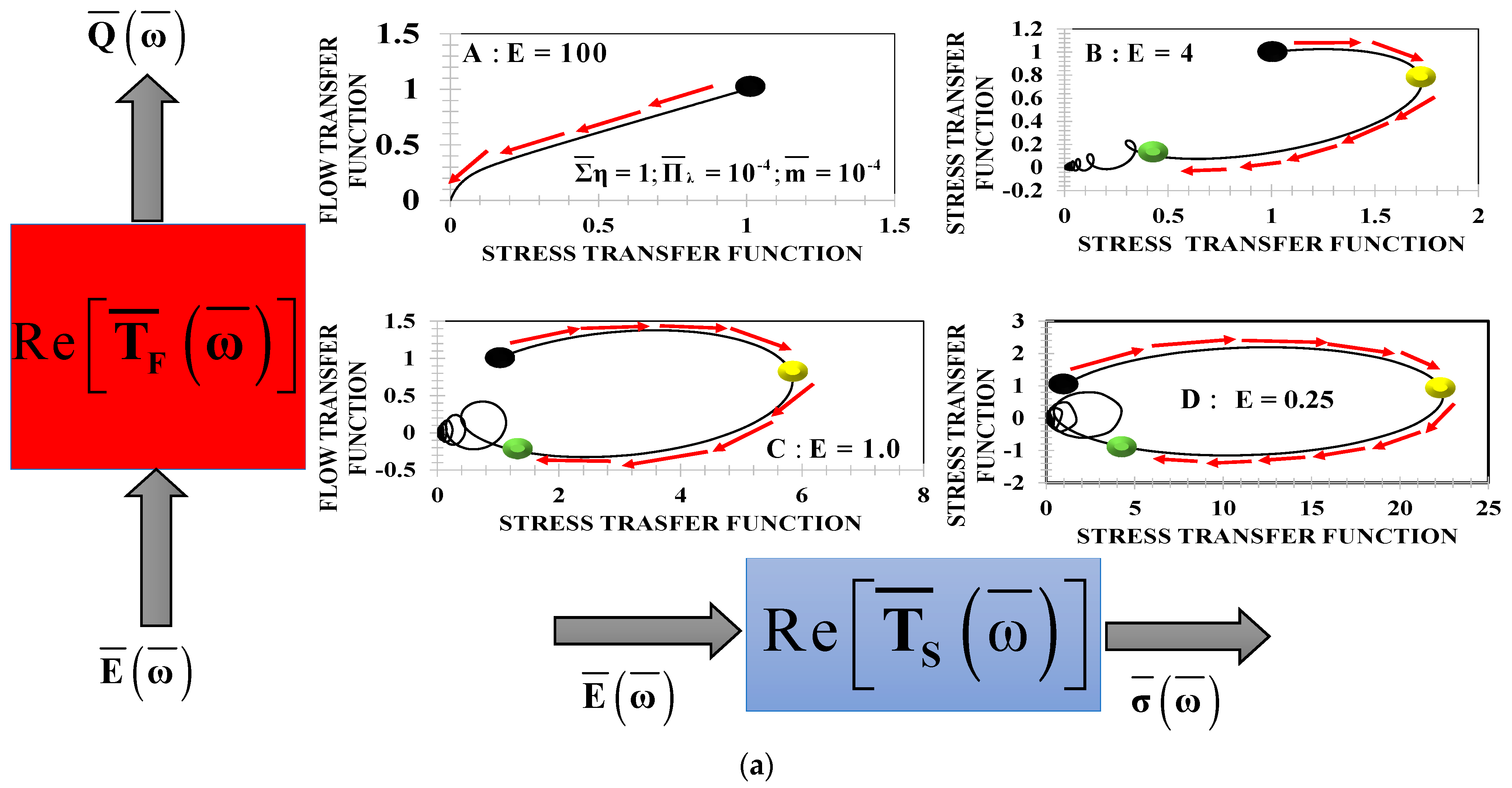
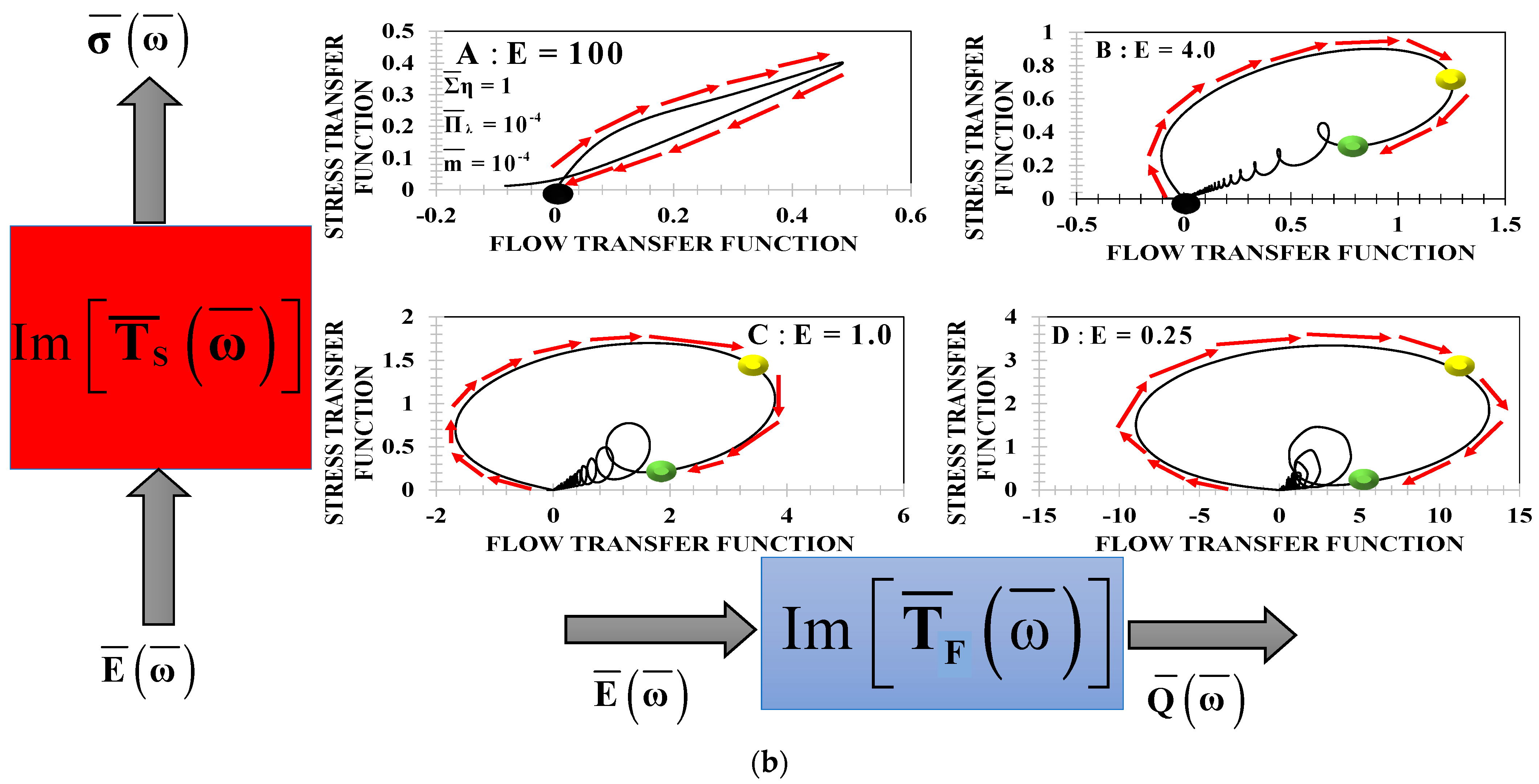
5.4. Flow-Stress Loop Diagrams

Figure 11 shows the norms of stress transfer STF vs. flow transfer FTF functions for Elastic E numbers: {(i) 100, (ii) 4, (iii) 1.0}. The numerical value of dimensionless numbers used in the simulation are the same of Figure 9a. Panel A: At high values in Elastic’s number and small frequency, the FTC and STF have the same numerical value (black circle). When the frequency increases, both transfer functions show decreasing behavior, up to an asymptotic value of zero. Panel B: In contrast, when the viscoelasticity increases through the E number, i.e., E = 4, the system has the same values at small frequencies. However, when it increases, the stress transfer function increases as a function of the flow transfer function (transition from the black to yellow point). At a critical frequency (stress saturation point: yellow color), the stress and flow decrease as a function of the frequency, and for a threshold frequency (green color), it seems to be a transition from the real and complex roots of the coupled STF-FTF device, and it starts to oscillate as a consequence of the resonance behavior of the system (See Appendix E). Panel C shows the STF—FTF response with an Elastic number E = 1.0. The black circle deals with the behavior at small frequencies, i.e., Lim ω ¯ →0, the black point is localized in the point (STF, FTF) = (1,1). When the dimensionless frequency increases, the STF and FTF show monotonically increasing behavior until a maximum value, followed by a stress saturation returning point (yellow color). This turning point coincides with the dominant resonance peaks (green color of the FTF and STF), which is associated with the mean Maxwell relaxation time. In the range of small and moderate frequencies, i.e., ω ¯ ∈ [1,10], there is a critical frequency (green point) where the system starts to oscillate and the coupled transfer functions show a multivalued function in the dynamical response. From a mathematical point of view, a plausible explanation of these oscillations deals with the ratio of the Bessel modified function of the first and second kind; it is possible that the system undergoes transitions from real to imaginary roots (See Appendix F for the mathematical details of the complex roots). The key physical message of Figure 11 is that the viscoelasticity, bulk-viscous, bulk-elastic, and flexoelectric behavior control the shape and orientation of the force–flow loops in the system.

5.5. Force–Flow Loops: Resonances and Transitions

Figure 12 summarizes key findings regarding resonances and monotonic-oscillatory transitions. Panels A, B show the flow, stress function as a function of frequency. Panel C shows the flow–force loop (See Appendix D for real and imaginary loops). The material conditions are as in Figure 10 and Figure 11. Here, the value of the elastic number is E = 1.
Figure 12 shows the following important points:
(a)
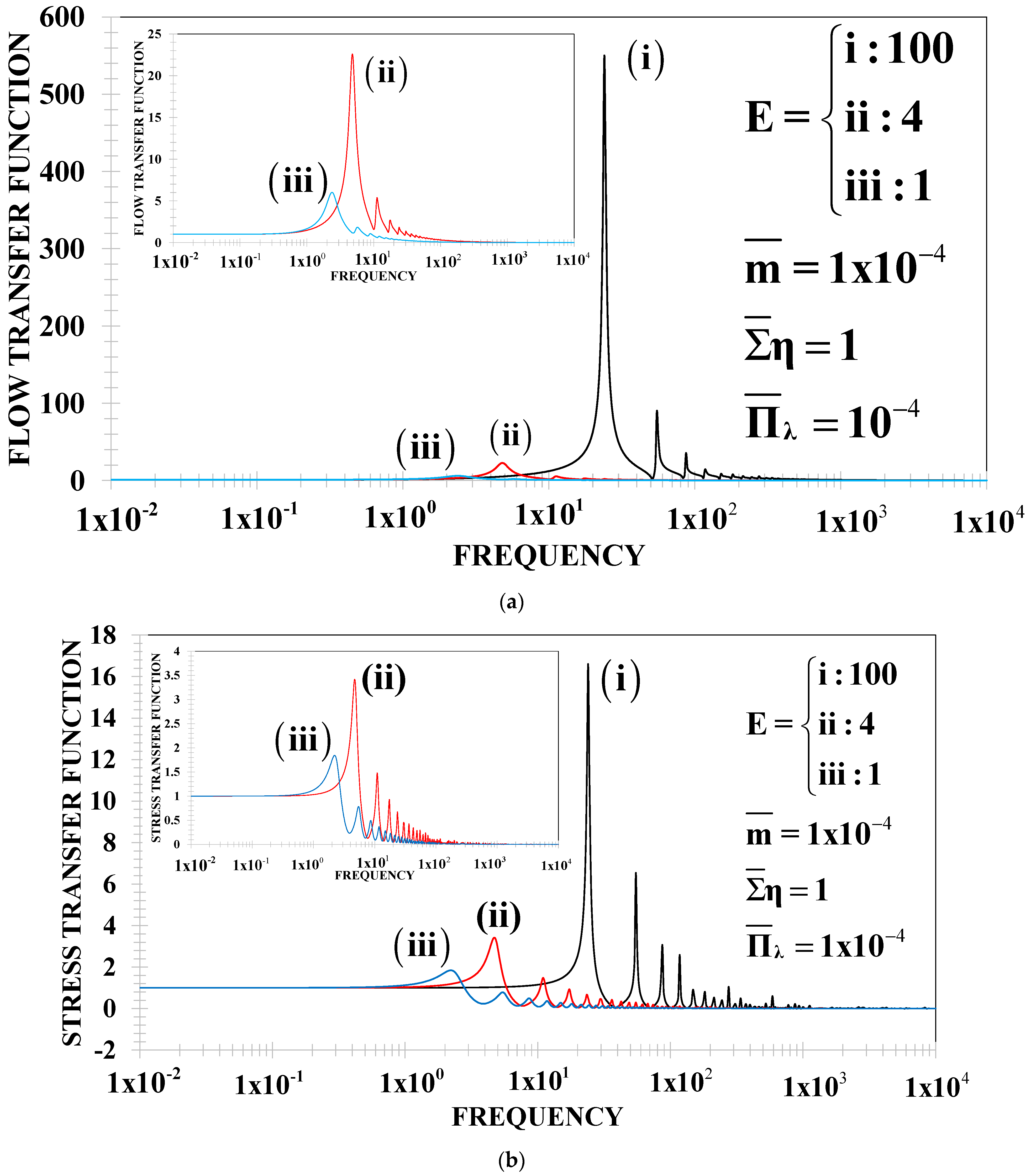
The material conditions needed to observe multiple resonance peaks in the FTF spectrum are: (i) an asymmetry in the viscoelastic liquid phases, i.e., one of them is totally viscoelastic and the other weakly viscoelastic, i.e., Π ¯ λ = ε , ε << 1. This means that one of the viscoelastic relaxation times is close to the unit λ ¯ L = 1 ε , and the other one is very small, ε =1 × 10⁻⁴. (ii) The system has large viscosity, i.e., Σ ¯ η = 1 . (iii) The membrane elasticity m = ε = 1 × 10⁻⁴. (iv) E is greater than zero, i.e., viscoelastic mechanisms (Weissenberg number We) (viscoelastic forces) dominate over the inertial and viscous forces (Reynolds number Re), E = We/Re > 0.
(b)
The maximum resonance peak is linked to the inertia, viscoelastic, and flexo-elastic processes, and its magnitude depends on the elastic number E = We/Re.
(c)
The multiple peaks are associated with a possible change in the roots of the ratio of the Bessel functions from real to complex values. The nature of these oscillations depends on coupled mechanisms associated with the inertia, viscous, elastic, and flexoelectric through the dimensionless numbers.
(d)
The global peak is found at a critical frequency whose value depends on the main Maxwell relaxation time, and this time is related with the frequency through ω ¯ peak = 1 / 1 ε . The secondary peak corresponds to the less dominant relaxation time, i.e., ω ¯ peak = 1 / ε .
(e)
The adequate model to predict resonance behavior is a new asymmetric rheological model, which is a variant of Burgers’ constitutive equation (Equation (10)). Other models (Jeffreys, Burgers, fractional derivative models) contribute to modify the resonance behavior through the viscosity operator defined in Equations (11) and (12) [3,4].
(f)
Multiple resonance peaks are found in other biological and complex systems [39,40]. For example, in biorheology, the pulsating pressure-driven force increases the volumetric flow, and its effect is dominated by dynamic permeability [41,42,43,44,45]. In veins with central and peripherical occlusions [46], the frequency can be tuned to obtain the maximum pulsating volumetric flow rate [46], as well as in oil recovery operations with surfactants such as worm-like micellar solutions [13,47,48,49,50].
(g)
The train of peaks can contribute to increase the FTF and STF, which are a starting point to study OHCs of mammalians and ear diseases [3,4,24,41].

6. Conclusions

The merit of this research is to propose a new asymmetric electro-rheological model (Equation (10)) to understand the dynamical behavior of flexoelectric membranes immersed in liquid viscoelastic media. The key issue is to understand the interactions between the driven electrical force (input), the volumetric flow rate, and the wall stress (outputs). This methodology is general and can be extended to include a higher viscoelastic linear and fractional model through the new asymmetric fluidity operator. The new asymmetric fluidity operator (Equation (12)) led us to obtain resonance behavior for the flow and stress transfer linear functions through macroscopical forces such as (i) inertia, (ii) bulk-viscous, (iii) bulk-elastic, (iv) flexoelectric, and (v) membrane elasticity in the physical system. This new approach has a particular parallel mechanical configuration (Maxwell/Hook/Maxwell) and its respective rheological equations of state (the Burgers-like model). The resonance behavior is totally controlled by the asymmetry of the viscoelastic phases, through fundamental dimensionless numbers (Appendix B). The new approach in this research is the elastic number (Equation (28)), which led us to display a power spectrum with one dominant resonant peak and a train of tunable secondary peaks. Lastly, special attention was placed on formulating and implementing an engineering device methodology that integrates design/control/prediction [3,4,5,10,11,12].

Author Contributions

E.E.H.-V. worked on the mathematical model of the system, A.D.R. conceived and design the theoretical analysis and material modeling, and he also supervised and co-wrote the paper. All authors have read and agreed to the published version of the manuscript.

Funding

A.D.R. was supported by the Natural Science and Engineering Research Council of Canada (NSERC), Compute Canada, Calcul Quebec, and McGill University. EEHV was supported by PAPIIT project no. IN102823 from DGAPA/UNAM, respectively.

Institutional Review Board Statement

Not applicable.

Informed Consent Statement

Not applicable.

Data Availability Statement

The numerical data that support the finding of this study are available from the corresponding author upon reasonable request.

Acknowledgments

A.D.R. gratefully acknowledges financial support of the Natural Science and Engineering Research Council of Canada (NSERC), Compute Canada, Calcul Quebec, and McGill University. EEHV gratefully acknowledges financial support of PAPIIT project no. IN102823 from DGAPA/UNAM. EEHV thanks Fausto Calderas from FESZ-UNAM for his critiques and comments and for his help in reviewing the manuscript. EEHV dedicates this research project to the memory of my beloved father “El ave de las tempestades”, Emilio Herrera Caballero, and my mother Marisela Valencia.

Conflicts of Interest

The authors declare no conflict of interest.

Abbreviations

Notation
aRadius of the pipe [m]
cfMembrane flexoelectric coefficient [C]
{C1, C2}Constants [1]
E (ω)Frequency-input electrical field [N/C]
E0Amplitude of the electrical field [N/C]
F (ω)Fourier transform
ezUnit vector [1]
F(t)Fourier transform
GElastic flexoelectric membrane [Pa]
Gb, GtElastic moduli defined in the bottom and the top [Pa]
hHeight of the spherical dome [m]
H(t)Average membrane curvature [m−1]
J0Bessel function of the first kind [1]
Y0Bessel function of the second kind [1]
k0, k1Membrane bending rigidity and torsion elastic moduli [J]
KDynamic permeability
LCharacteristic axial length of the capillary [m]
mElastic ratio [1]
Q (ω)Output volumetric flow rate [m3/s]
Δp(z,t)Pressure, constant pressure at z = 0 and z = 2L, and pressure difference [Pa]
PR, pLPressure defined at the top and the bottom [Pa]
p0Constant pressure at the top in the bottom [Pa]
Q(t)Volumetric flow rate [m3/s]
Q (ω)Frequency-volumetric flow rate [m3/s]
QR(t), QL(t)Top and bottom volumetric flow rate [m3/s]
rRadial coordinate [m]
Re [TF (ω)]Real part of the transfer function [m3s−1/NC−1]
Im [TF (ω)]Imaginary part of the transfer function [m3s−1/NC−1]
TF (ω) Complex flow transfer function [m3s−1/NC−1]
TS (ω) Complex stress transfer function [m3s−1/NC−1]
tTime coordinate [s]
tiInertial time [s]
VzAxial velocity [m/s]
Operators
Dt = ∂/∂tTime differential operator [1/s]
OΦ(Dt)Viscosity operator [Pas]
R(Dt), OηL(Dt)Right and left viscosity operators [Pas]
Other symbols
(r,ϕ,z)Cylindrical coordinates [m,1, m]
Shape factor [1/m2]
Dyadic product [1]
Gradient operator [1/m]
ΔDelta operator [1]
Vectors and tensors
DRate of deformation tensor [1/s]
EElectrical field vector [N/C]
GAcceleration of the gravitational forces [m/s2]
kOuter unit normal vector [1]
kkDyadic product of the outer unit normal vector [1]
TTotal stress tensor [Pa]
IUnit tensor [1]
VVelocity field [ms−1]
VVelocity gradient [s−1]
ΔDelta [1]
Greek vectors and tensors
σTotal stress tensor [Pa]
σR, σLRight and left stress tensors [Pa]
σMMembrane stress tensors [Pa]
σwWall stress [Pa]
Greek letters
βComplex wave vector [1/m]
εSmall parameters [1]
ρxDensity of the viscoelastic liquid phases [kg/m3]
γ0Interfacial surface tension at zero electric field [F/m]
γTotal shear strain in the system [1]
γtTop deformation of the Maxwell element [1]
γbBottom deformation of the Maxwell element [1]
γ0Interfacial surface tension at zero electric field [F/m]
ηL, ηRLeft and right viscosities [Pas]
λL, λRLeft and right viscoelastic relaxation times [s]
σrzrz component of the shear stress tensor [Pa]
ωAngular frequency [rad/s]
ΣρTotal liquid density [kg/m3]
ΣGTotal bulk elasticity [Pa]
ΣλTotal Maxwell relaxation times [s]
ΣηTotal bulk viscosities [Pas]
ΦEElectrical potential [J/C]
Dimensionless variables
C ¯ 1 , C ¯ 2 Constants [1]
r ¯ Radial coordinate [1]
t ¯ Process time [1]
V ¯ z Axial velocity [1]
E ¯ z Electric field [1]
Q ¯ Volumetric flow rate [1]
G ¯ Elastic membrane [1]
ω ¯ Frequency [1]
σ ¯ Viscoelastic shear stress [1]
σ ¯ F E Flexoelectric stress [1]
O ¯ Φ Fluidity operator [1]
Dimensionless numbers
EElastic [1]
DeDeborah [1]
WoWomersley [1]
m ¯ Membrane elastic ratio [1]
Σ ¯ η Elastic ratio [1]
Π ¯ λ Memory [1]
Other symbols
(r,ϕ,z)Cylindrical coordinates [m,1, m]
e−iωtComplex negative exponential function [1]
πPi constant [1]
∂Vz/∂r Shear strain [1/s]
{∂/∂z, ∂/∂t} Spatial and temporal time derivatives [m−1,s−1]
|·|Absolute value [1]
Subscripts
{L, R}Refers to the left and the right fluids [1]
Superscripts
( )TRefers to the transport of a tensor [1]
Abbreviators
LCLiquid crystal
NLCNematic liquid crystal
OHCOuter hair cell
SAOSSmall amplitude oscillatory shear

Appendix A

To avoid unnecessary repetitions of lengthy definitions and to increase readability, we include a nomenclature at the end of these appendices.

Dimensionless Variables

The following dimensionless variables are proposed for the frequency, radial coordinate, z-coordinate, process time, shear stress, flexoelectric shear stress, axial velocity electric field, electric potential, fluidity operator, volumetric flow rate, right and left volumetric flow rates, compliance, membrane elasticity, complex moduli, constants {C1 C2}, and average membrane curvature
ω   ¯ = Σ λ ω ;   r ¯ = r a ; z ¯ = z L ; t ¯ = t Σ λ ; σ ¯ = σ Σ G ; σ ¯ F E = σ F E Σ G ; V ¯ z = V z a c f Σ G Σ λ E 0 ; E ¯ z = Ez E 0 ; Φ ¯ = Φ Φ 0 ; O ¯ Φ = O Φ 1 / Σ G Σ λ ; Q ¯ = Q π a 3 / Σ λ ; Q ¯ R = Q R π a 3 / Σ λ ; Q ¯ L = Q L π a 3 / Σ λ ; J ¯ = J 1 / Σ G ; G ¯ = G Σ G ; G ¯ * = G * Σ G ; C ¯ 1 = C 1 a / Σ λ ; C ¯ 2 = C 2 a / Σ λ ; H ¯ = a H
The material parameters are:
η ¯ R = η R Σ η ; η ¯ L = η L Σ η ; λ ¯ R = λ R Σ λ ; λ ¯ L = λ L Σ λ ; G ¯ = G Σ G ; G ¯ R = G R Σ G ; G ¯ L = G L Σ G
Equation (A2) satisfies:
λ ¯ R + λ ¯ L = 1   ; G ¯ R + G ¯ L = 1
The dimensionless elastic ratio m ¯ is defined as:
m ¯ = G ¯ 1 + G ¯
The selection of these characteristic variables involves: (i) total viscosity, (ii) total relaxation times, and (iii) total bulk fluid elasticity. These variables’ specifications allow us to tune internal (inertial, viscous, and viscoelastic) and external characteristic mechanisms (frequency, electrical field).

Appendix B

The purpose of this appendix is to show the key explanations needed to perform the dimensionless numbers analysis of the present model (Equations (9)–(12)) and derive the mechanical network model, block diagram, and transfer functions, respectively.

Parametric Material Space

The dimensionless numbers deduced in the flow and stress transfer functions are given by:
(i) Memory Π ¯ λ = λ ¯ R λ ¯ L : obeys λ ¯ R + λ ¯ L = 1 and defines the elastic asymmetry of the fluids. When Π ¯ λ < < 1 (highly asymmetric case) one of the fluids is nearly inelastic, and when Π ¯ λ = 1 / 4 (highly symmetric case) both fluids are equally elastic. (ii) Bulk viscous Σ ¯ η = G ¯ L λ ¯ L + G ¯ R λ ¯ R : total viscosity in the system, where the elastic dimensionless moduli satisfy G ¯ L + G ¯ R = 1 . (iii) Elastic ratio m ¯ : dimensionless ratio between the membrane and the total system elasticity: m ¯ ∈ (0, 1). A floppy (soft) and stiff (rigid) membrane corresponds to m ¯ < < 1 and m ¯ 1 , respectively. The fourth group is a ratio between the flexoelectric and bulk elastic mechanisms, and it is given by:
Q r = a c f E 0 / 4 L Σ G
When Qr > 1, the flexoelectric forces dominate over the bulk elastic mechanisms, whereas when Qr < 1, the bulk-elastic forces dominate the process. Finally, the elastic number E:
E = W e Re = Σ λ Σ ρ a 2 / Σ G Σ λ
E is the ratio between two fundamental and crucial dimensionless numbers called the Weissenberg and Reynolds numbers associated with the viscoelasticity and viscous-inertial forces. The wavelength vector deals with the pulsating Womersley number associated with the competition between the viscous-oscillatory mechanisms [42,43].
W 0 2 = a 2 Σ ρ Σ η ω = t v ω
In Equation (A7), tv is the inertial time-scale used in the Newtonian case. Equation (A8) can be expressed in terms of the viscoelastic mechanisms though the total viscoelastic characteristic time tv = Σλ [3,4]:
W 0 = t v t v e t v e ω = 1 t v e / t v t v e ω = E 1 / 2 ω ¯
Equation (A8) relates the Womersley number Wo used in biofluid mechanics with the elastic ratio numbers. Wo deals with the pulsatile flow frequency and the dissipation associated with the viscous effects [42,43].

Appendix C

To avoid unnecessary repetitions of lengthy definitions and to increase readability, we include a nomenclature at the end of these appendices.

Appendix C.1. Transfer Function

This derivation can be generalized to any particular viscoelastic and viscoelastic fractional Maxwell. Defining the balance shape equation of the liquid crystal membrane in the following form:
c f Ez t = k k : Δ T b = Δ p t + G H t
Equation (A9) is a classical balance force shape equation; E (t) is the electrical field, cf is the electric constant, ℑ is the inverse of the characteristic area, Δp(t) is the pressure difference, G is the flexoelectric-elastic membrane, and H(t) is average membrane curvature. Taking the Fourier transforms of the shape equation (Equation (A10)) and using the Poiseuille viscoelastic flow (Equation (41)) and coupling the speed of the average membrane curvature:
Q t = 1 2 π a 4 d H t d t
Equation (A11) yields the block diagram shown in Figure A1a. In what follows, we analyze the three elements shown in the block diagram (Figure A1a): (i) flexoelectric transfer function, (ii) rheological transfer function, and (iii) time operator.
Figure A1. (a). Block diagram for a power conversion device based on flexoelectric membranes. Three important blocks are (i) flexoelectric transfer function (middle left box), (ii) rheological transfer function (top box), and (iii) time operator (bottom right box). The flexoelectric transfer function is a SIDO (single input–dual output) block, while the other two are SISO (single input–single output blocks). (b). Effective block diagram for the flexoelectric membrane embedded in two viscoelastic media.
Symmetry 15 01004 g0a1

Appendix C.2. Flexoelectric Transfer Function

The flexoelectric transfer function cfℑE0G converts the Ez(ω) input into membrane curvature H(ω) and pressure drop Δp(ω):
E ¯ z ω ¯ I n p u t Q R SIDO   Block = Δ ¯ p ω ¯ + G ¯ H ¯ ω O u t p u t = Δ ¯ p ω ¯ + m ¯ 1 m ¯ H ¯ ω O u t p u t
In Equation (A11), the pressure difference, external force, average membrane curvature, and membrane elasticity are defined:
Δ p ¯ = Δ p 4 L Σ G / a ; E ¯ z = E ¯ z E 0 ; H ¯ = a H
The dimensionless numbers are given by:
Q r = a c f E 0 / 4 L Σ G ;   G ¯ = G Σ G = m ¯ 1 m ¯
Interestingly, this is a SIDO (single input–dual output) block, and it encapsulates the integrated nature of membrane fluctuations and viscoelastic flow. This transfer function is the ratio between the flexoelectric and bulk-elastic forces, since the conversion depends on the effective bulk-elastic mechanisms.

Appendix C.3. Time Operator: Electrical Field

Applying the dimensionless time operator i ω ¯ to Equation (A11), the following expression is obtained:
i ω ¯ E ¯ z ω ¯ I n p u t Q r SIDO   Block = i ω ¯ Δ ¯ p ω ¯ O u t p u t + m ¯ 1 m ¯ i ω ¯ H ¯ ω ¯ O u t p u t
This transfer function is the ratio between the flexoelectric and bulk-elastic forces, since the conversion depends on the effective bulk-elastic mechanisms, as shown in Figure A1a. It is important to note that there are two outputs here; one refers to pressure Δ p ¯ ω ¯ , and the other to curvature H ¯ ω ¯ .

Appendix C.4. Rheological Transfer Function

The evolution of the average membrane curvature causes an inertia-viscoelastic Poiseuille volumetric flow Q ¯ p ω ¯ , which is regulated by the material function through a complex viscoelastic material function Oη(ω) (Figure A1a):
i ω ¯ Δ ¯ p ω ¯ I n p u t i 2 Q r 1 2 i ω ¯ Κ β ¯ ω ¯ , E O ¯ η ω ¯ S I S O   B l o c k = i ω ¯ Q ¯ p ω ¯ O u t p u t
Interestingly, this is a SISO (single input–single output) block, and it shows how pressure drops create viscoelastic flow in Equation (A15) and O ¯ η ω ¯ is a general viscosity operator function defined. Κ β ¯ ω ¯ , E can be interpreted as a dynamic permeability, and it is given in terms of Bessel functions:
Κ β ¯ ω ¯ , E = 8 i 2 β ¯ 2 ω ¯ , E 1 J 1 β ¯ ω ¯ , E / β ω ¯ , E J 0 β ω ¯ , E
In Equation (A16), the dimensionless parameter β ¯ ω ¯ , E is the same as Equation (41) for the system. In partial summary, this block transforms a pressure signal into a flow rate signal (Equation (A16)), which is at the core of power generation.

Appendix C.5. Time Operator: Average Membrane Curvature

At the bottom right of Figure A1a, we find this SISO block that converts curvature changes into volumetric flow. The dimensionless average membrane curvature
i 2 2 i ω ¯ H ¯ ω ¯ I n p u t = Q ¯ M ω ¯ O u t p u t
The volumetric Poiseuille flow Q ¯ P ω ¯ and the membrane volumetric flow rate Q ¯ M ω ¯ are the same, i.e., Q ¯ P ω ¯ = Q ¯ M ω ¯ = Q ¯ ω ¯ . Combining Equations (A13)–(A15):
Q ¯ ω ¯ = i 2 Q r 1 m ¯ m ¯ i ω ¯ 1 + 1 m ¯ m ¯ i ω ¯ O ¯ η i ω ¯ / Κ β ¯ ω ¯ , E E ¯ z ω ¯
In Equation (A18), Qr = acfℑE0L−1G is a ratio between the flexoelectric and bulk elastic forces. A particular case of Equation (A16) is obtained when it is considered a floppy membrane, i.e., m ¯ << 1, so the above equation is simplified to the following analytical expression:
Q ¯ ω ¯ = i 2 Q r 1 m ¯ m ¯ i ω ¯ 1 + 1 m ¯ m ¯ i ω ¯ O ¯ η i ω ¯ / Κ β ¯ ω ¯ , E E ¯ z ω ¯ i 2 Q r Κ β ¯ ω ¯ , E O ¯ η i ω ¯ E ¯ z ω ¯
Equation (A19) represents the volumetric flow of the viscoelastic system, which is a consequence of the dynamical linear response of the system Κ β ¯ ω ¯ , E , the rheology of the system, through the viscosity operator, the driven force E ¯ z ω ¯ , and, finally, a ratio between the flexoelectric and bulk-elastic mechanisms.

Appendix C.6. Total Transfer Function

From Equation (A19)
T ¯ F ω ¯ = Re [ T ¯ F ω ¯ ] + i Im [ T ¯ F ω ¯ ] = Q ¯ ω ¯ E ¯ z ω ¯ = i 2 Q r 1 m ¯ m ¯ i ω ¯ 1 + 1 m ¯ m ¯ i ω ¯ O ¯ η i ω ¯ / Κ β ¯ ω ¯ , E
In partial summary, this section presents the required sequence of calculations to build the block diagram of Figure 12a that complements the mechanical network model in Figure 6 and provides an alternative total transfer function that forms the basis of the eventual control of these power devices. Using the same arguments as Equation (A17), the following expression is obtained:
T F ω ¯ = Re [ T F ω ¯ ] + i Im [ T F ω ¯ ] = Q ¯ ω ¯ E ¯ ω ¯ i 2 Q r Κ β ¯ ω ¯ , E O ¯ η ω ¯
Equation (A21) reduces to Equations (44) and (45), which was previously obtained from thermodynamic and rheologic considerations.

Appendix D

Real and Imaginary Flow–Stress Loops
Figure A2a,b show the following important characteristics:
(a)
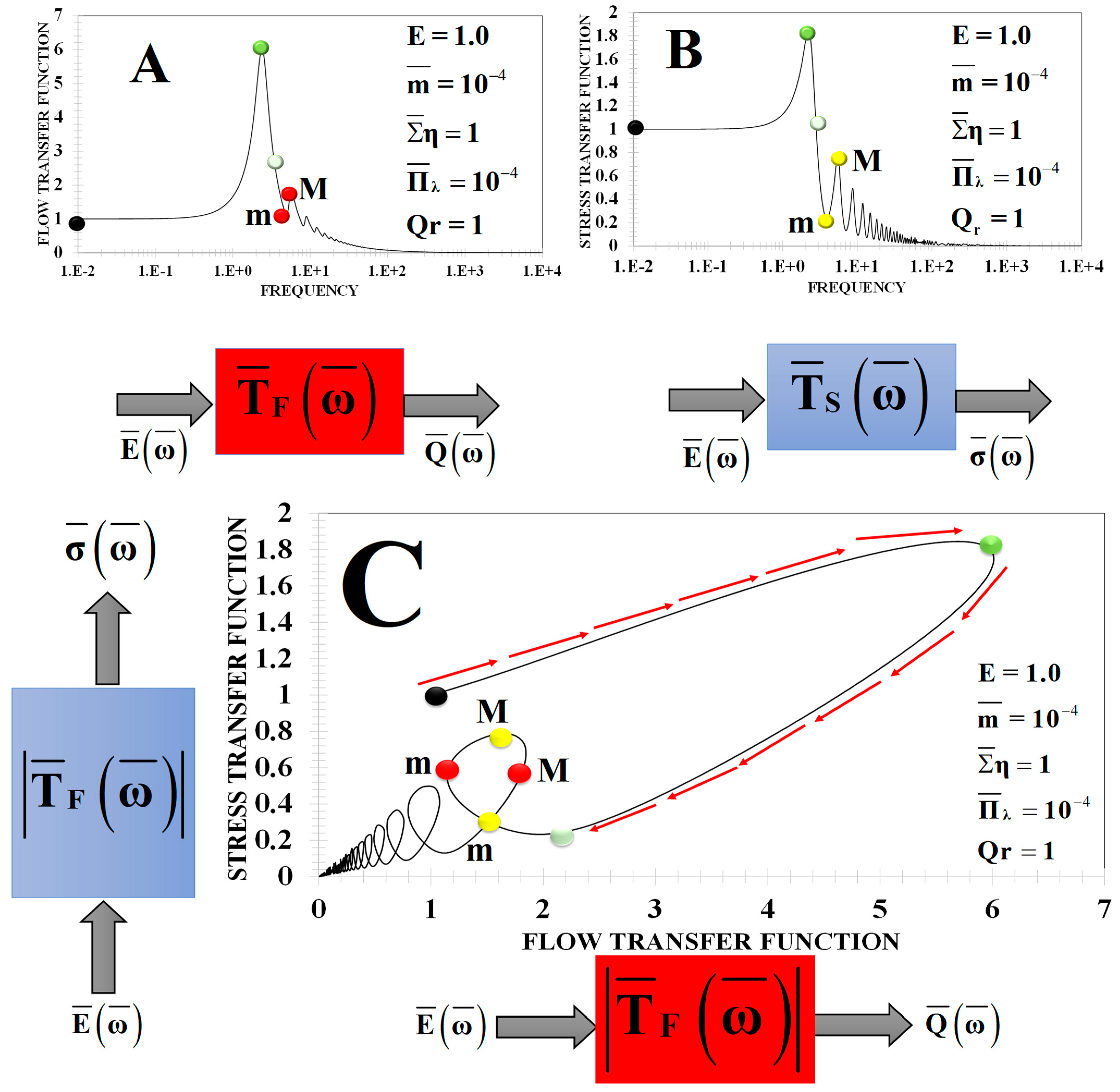
The stress and flow transfer functions are coupled and for a critical frequency, where the system shows a stress saturation (peak resonance);
(b)
The viscoelastic forces control the shape, magnitude, and orientation of the force–flow loops;
(c)
At small frequency, the real stress and flow transfer functions have the same magnitude, at a value 1 (membrane mode); hence, the imaginary part of the stress and flow rate starts from zero value.
Figure A2. (a). Real values corresponding to Figure 12. (b). Imaginary values corresponding to Figure 12.
Symmetry 15 01004 g0a2aSymmetry 15 01004 g0a2b

Appendix E

Figure A3 shows a summary of the key issues and contributions of this research.
Figure A3. Schematic summary of the present research.
Symmetry 15 01004 g0a3
The complex viscosity (inverse of the fluidity operator) displays three important regions: (i) flexo-viscous, (ii) flexo-viscoelastic, and (iii) flexo-bulk-elastic mechanisms (Letter A). The resonances and biological zone for outer hair cells is given in the flexo-viscoelastic region. The triangle (Letter B) shows the main material conditions to have resonance behavior. Only the three modes lead us to the dominant and resonance peaks. Finally, the 3D-parametric space shows the effect of the elastic ratio. When m goes to one, i.e., the system shows a parallel line. Here, the flexoelectric membrane is a Hooke solid.

Appendix F

In this appendix, the roots of the beta parameter are studied. The beta parameter can be expressed in the following form:
β ¯ 2 i ω ¯ = E 1 i ω ¯ O Φ i ω ¯
and
O ¯ Φ i ω ¯ = 1 m ¯ 1 Π λ ω ¯ 2 i ω ¯ ω ¯ 2 m ¯ Π λ ω 2 + m ¯ + 1 m ¯ Σ ¯ η i ω ¯
From (A23), the real and imaginary parts
O ¯ Φ i ω ¯ = 1 m ¯ ω ¯ 2 1 Π ¯ λ ω ¯ 2 m ¯ + 1 m ¯ Σ ¯ η m ¯ Π ¯ λ ω ¯ 2 m ¯ Π ¯ λ ω ¯ 2 2 + ω ¯ m ¯ + 1 m ¯ Σ ¯ η 2 + ω ¯ 1 Π ¯ λ ω ¯ 2 m ¯ Π ¯ λ ω ¯ 2 + ω ¯ m ¯ + 1 m ¯ Σ ¯ η m ¯ Π ¯ λ ω ¯ 2 2 + ω ¯ m ¯ + 1 m ¯ Σ ¯ η 2 i
Once the numerical values of the groups defined in Figure 9 are substituted into Equation (A24), the fluidity operator can be separated into a real complex contribution:
O ¯ Φ i ω ¯ = Re O ¯ Φ i ω ¯ + iIm O ¯ Φ i ω ¯ = ω ¯ 2 1 m ¯ Π λ ω ¯ 2 2 + ω ¯ 2 + ω ¯ m ¯ Π ¯ λ ω ¯ 2 + Π ¯ λ ω ¯ 2 2 + ω ¯ m ¯ Π λ ω ¯ 2 2 + ω ¯ 2 i
Therefore, the square of the beta parameter is given by:
β ¯ 2 i ω = E 1 i ω ¯ O ¯ Φ i ω ¯ = E 1 ω ¯ 2 m ¯ Π ¯ λ ω ¯ 2 + Π ¯ λ ω ¯ 2 2 + ω ¯ m ¯ Π ¯ λ ω ¯ 2 2 + ω ¯ 2 + E 1 ω ¯ 3 1 m ¯ Π ¯ λ ω ¯ 2 2 + ω ¯ 2 i
and
β ¯ i ω ¯ = R ω ¯ + I ω ¯ i
where the real and imaginary parts are given by the following expression:
R ω ¯ = E 1 ω ¯ 2 m ¯ Π ¯ λ ω ¯ 2 + Π ¯ λ ω ¯ 2 2 + ω ¯ m ¯ Π ¯ λ ω ¯ 2 2 + ω ¯ 2 ;   I ω ¯ = E 1 ω ¯ 3 1 m ¯ Π ¯ λ ω 2 2 + ω ¯ 2
The complete solution:
β ¯ ω ¯ = R ω ¯ + i I ω ¯ = ± R ω ¯ + R 2 ω ¯ + I 2 ω ¯ 2 + R ω ¯ + R 2 ω ¯ + I 2 ω ¯ 2 i , I ω ¯ > 0
The second case:
β ¯ ω ¯ = R ω ¯ + i I ω ¯ = ± R ω ¯ + R 2 ω ¯ + I 2 ω ¯ 2 R ω ¯ + R 2 ω ¯ + I 2 ω ¯ 2 ; I ω ¯ < 0
According to our case, the imaginary part of complex wave vector β ¯ ω ¯ is negative, so Equation (A30) must be used to analyze the physics of the system.

References

  1. Wang, Z.; Servio, P.; Rey, A.D. Pattern formation, structure and functionalities of wrinkled liquid crystals surfaces: A soft matter biomimicry platform. Front. Soft Matter 2023, 3, 1123324. [Google Scholar] [CrossRef]
  2. Petrov, A.G. The Lyotropic State of Matter: Molecular Physics and Living Matter Physics; Gordon and Breach Science Publisher: Amsterdam, The Netherlands, 1999. [Google Scholar]
  3. Herrera-Valencia, E.E.; Rey, A.D. Electrorheological model based on liquid crystals membranes with applications to outer hair cells. Fluids 2018, 3, 35. [Google Scholar] [CrossRef]
  4. Herrera-Valencia, E.E.; Rey, A.D. Mechano-electric transduction performance of actuation device based on liquid crystal membrane flexoelectricity. Phil. Trans. R. Soc. A 2014, 372, 20130369. [Google Scholar] [CrossRef]
  5. Rey, A.D. Nonlinear actuator model for flexoelectric membranes. Int. J. Des. Nat. Ecodynam. 2008, 3, 28–38. [Google Scholar] [PubMed]
  6. Petrov, A.G. Flexoelectricity of model and living membranes. BBA-Biomembr. 2001, 1561, 1–25. [Google Scholar] [CrossRef] [PubMed]
  7. Petrov, A.G. Electricity and mechanics of biomembrane systems: Flexoelectricity in living membranes. Anal. Chim. Acta 2006, 568, 70–83. [Google Scholar] [CrossRef]
  8. Lee, D. Flexoelectricity in thin films and membranes of complex solids. APL Mater. 2020, 8, 090901. [Google Scholar] [CrossRef]
  9. Rey, A.D.; Servio, P.; Herrera-Valencia, E.E. Stress-Sensor Device Based on Flexoelectric Liquid Crystalline Membranes. ChemPhysChem 2014, 15, 1405–1412. [Google Scholar] [CrossRef]
  10. Rey, A.D.; Servio, P.; Herrera-Valencia, E.E. Bioinspired model of mechanical energy harvesting based on flexoelectric membranes. Phys. Rev. E 2013, 87, 022505. [Google Scholar] [CrossRef]
  11. Rey, A.D. Linear viscoelastic model for bending and torsional modes in fluid membranes. Rheol. Acta 2008, 47, 861–871. [Google Scholar] [CrossRef]
  12. Aguilar-Gutierrez, O.F.; Herrera-Valencia, E.E.; Rey, A.D. Generalized Boussinesq-Scriven surface fluid model with curvature dissipation for liquid surfaces and membranes. J. Coll. Int. Sci. 2017, 503, 103–114. [Google Scholar] [CrossRef] [PubMed]
  13. Wang, Z.; Servio, P.; Herrera-Valencia, E.E.; Rey, A.D. Thermal fluctuation spectrum of flexoelectric viscoelastic semiflexible filaments and polymers: A line liquid crystal model. Can. J. Chem. Eng. 2022, 100, 3162–3173. [Google Scholar] [CrossRef]
  14. Rabbitt, R.D.; Clifford, S.; Breneman, K.D.; Farrell, B.; Brownell, W.E. Power efficiency of outer hair cell somatic electromotility. PLoS Comput. Biol. 2009, 5, e1000444. [Google Scholar] [CrossRef] [PubMed]
  15. Dewey, J.W.; Altoe, A.; Shera, C.A.; Oghalai, J.S. Cochlear outer hair cell electromotility enhances organ of Corti motion on a cycle-by-cycle basis at high frequencies in vivo. Proc. Natl. Acad. Sci. USA 2021, 118, e2025206118. [Google Scholar] [CrossRef]
  16. Oghalai, J.S.; Zhao, H.B.; Kutz, J.W.; Brownell, W.E. Voltage-and tension-dependent lipid mobility in the outer hair cell plasma membranes. Science 2000, 287, 658–661. [Google Scholar] [CrossRef]
  17. Brownell, W.E. Evoked mechanical responses of isolated cochlear outer hair cells. Science 1985, 227, 194–196. [Google Scholar] [CrossRef] [PubMed]
  18. Levic, S.; Lukaskina, V.A.; Simoes, P.; Lukashkin, A.N.; Russell, I.J. A gap-junction mutation reveals that outer hair cell estracellular receptor potentials drive high-frequency cochlear amplification. J. Neurosci. 2022, 19, 7875–7884. [Google Scholar] [CrossRef]
  19. Altoe, A.; Shera, C.A. The long outer-hair-cell RC time constant: A feature, not a bug, of the Mammalian Cochlea. J. Assoc. Res. Otolaryngol. 2023, 24, 129–145. [Google Scholar] [CrossRef]
  20. Yeh, W.H.; Shubina-Oleinik, O.; Levy, J.M.; Pan, B.; Newby, G.A.; Wornow, M.; Burt, R.; Chen, J.C.; Holt, J.R.; Liu, D.R. In vivo base editing restores sensory transduction and transient improves auditory function in a mouse model of recessive deafness. Sci. Transl. Med. 2020, 12, eaay9101. [Google Scholar] [CrossRef]
  21. Torbati, M.; Mozaffari, K.; Liu, L.; Sharma, P. Coupling of mechanical deformation and electromagnetic fields in biological cells. Rev. Mod. Phys. 2022, 94, 025003. [Google Scholar] [CrossRef]
  22. Lahlou, G.; Calvet, C.; Giorgi, M.; Lecomte, M.J.; Safieddine, S. Towards the clinical application of gene therapy for genetic inner ear diseases. J. Clin. Med. 2023, 12, 1046. [Google Scholar] [CrossRef]
  23. Bowling, T.; Lemons, C.; Meaud, L. Reducing tectorial membrane viscoelasticity enhances spontaneous otoacoustic emissions and compromises the detection of low-level sound. Sci. Rep. 2019, 9, 7494. [Google Scholar] [CrossRef] [PubMed]
  24. Rabbitt, R.D. The cochlear outer hair cell speed paradox. Proc. Natl. Acad. Sci. USA 2020, 117, 21880–21888. [Google Scholar] [CrossRef] [PubMed]
  25. Mussel, M.; Schneider, M.F. It sounds like an action potential: Unification of electrical, chemical and mechanical aspects of acoustic pulses in lipids. J. R. Soc. Interface 2019, 16, 20180743. [Google Scholar] [CrossRef]
  26. Mao, X.; Shokef, Y. Introduction to force transmission by nonlinear biomaterials. Soft Matter 2021, 17, 10172–10176. [Google Scholar] [CrossRef] [PubMed]
  27. Ronceray, P.; Broedersz, C.P.; Lenz, M. Stress-dependent amplification of active force in non-linear elastic media. Soft Matter 2019, 15, 331. [Google Scholar] [CrossRef] [PubMed]
  28. Bird, R.B.; Armstrong, R.C.; Hassager, O. Dynamics of Polymeric Liquids; Fluid Mechanics Wiley: New York, NY, USA, 1977; Volume 1. [Google Scholar]
  29. Shankar, V.; Subramanian, G. A linear route to elasto-inertial turbulence. Sci. Talks 2022, 3, 100051. [Google Scholar] [CrossRef]
  30. Castillo-Sánchez, H.A.; de Souza, L.F.; Castelo, A. Numerical Simulation of Rheological Models for Complex Fluids Using Hierarchical Grids. Polymers. Polymers 2022, 14, 4958. [Google Scholar] [CrossRef]
  31. Castillo Sánchez, H.A.; Jovanovic, M.R.; Kumar, S.; Morozov, A.; Shakar, V.; Subramanian, G.; Wilson, H.J. Understanding viscoelasticity flow instabilities: Oldroyd Band beyond. J. Non-Newton. Fluid Mech. 2022, 302, 104742. [Google Scholar] [CrossRef]
  32. Jeonghun, N.; Hyunjung, L.; Dookon, K.; Hyunwook, J.; Sehyun, S. Continuous separation of microparticles in a microfluidic channel via the elasto inertial effect of non-Newtonian fluid. Lab Chip 2012, 12, 1347. [Google Scholar]
  33. Fernandez-Feria, R.; Alaminos-Quesada, J. Purely pulsating flow of a viscoelastic fluid in a pipe revisited: The limit of large Womersley number. J. Non-Newton. Fluid Mech. 2015, 217, 32–36. [Google Scholar] [CrossRef]
  34. Simpson, J.P.; Leylek, J.H. The influence of Womersley number on non-Newtonian effects: Transient computational study of blood rheology. J. Fluids. Eng. 2023, 145, 011206. [Google Scholar] [CrossRef]
  35. Loudon, C.; Tordesillas, A. The use of the dimensionless Womersley number to characterize the unsteady nature of internal flow. J. Theor. Biol. 1998, 191, 63–78. [Google Scholar] [CrossRef] [PubMed]
  36. Park, N.; Nam, J. Analysis of pulsatile shear-thinning flows in rectangular channels. Phys. Rev. Fluids 2022, 7, 123301. [Google Scholar] [CrossRef]
  37. Peralta, M.; Arcos, J.; Mendez, F.; Bautista, O. Mass transfer through a concentric annulus microchannel driven by an oscillatory electroosmotic flow of a Maxwell fluid. J. Non-Newton Fluid Mech. 2020, 279, 104281. [Google Scholar] [CrossRef]
  38. Rath, S.; Mahapatra, B. Low Reynolds number pulsatile flow of a viscoelastic fluid through a Channel: Effects of fluid rheology and pulsation parameters. J. Fluid Eng. 2022, 144, 021201. [Google Scholar] [CrossRef]
  39. Castro, M.; Bravo-Gutiérrez, M.E.; Hernández-Machado, A.; Corvera-Poiré, E. Dynamic characterization of permeabilities and flows in microchannels. Phys. Rev. Lett. 2008, 101, 224501. [Google Scholar] [CrossRef]
  40. Yañez, D.; Travasso, R.D.M.; Corvera-Poiré, E. Resonances in the response of fluidic networks inherent to the cooperation between elasticity and bifurcations. R. Soc. Open Sci. 2019, 6, 190661. [Google Scholar] [CrossRef]
  41. Flores, J.; Corvera-Poiré, E.; Del Rio, J.A.; López de Haro, M. A plausible explanation for heart rates in mammals. J. Theor. Biol. 2010, 265, 599. [Google Scholar] [CrossRef]
  42. Flores, J.; Alastruey, J.; Corvera-Poiré, E. A novel analytical approach to pulsatile blood flow in the arterial network. Ann. Biomed. Eng. 2016, 44, 3047–3068. [Google Scholar]
  43. Lindner, A.; Bonn, D.; Corvera-Poiré, E.; Ben Amar, M.; Meunier, J. Viscous fingering in non-Newtonian fluids. J. Fluid Mech. 2002, 469, 237–256. [Google Scholar] [CrossRef]
  44. Torres-Rojas, A.M.; Pagonabarraga, I.; Corvera-Poiré, E. Resonances of Newtonian fluids in elastomeric microtubes. Phys. Fluids 2017, 29, 122003. [Google Scholar] [CrossRef]
  45. Torres-Herrera, U. Dynamic permeability of fluids in rectangular and square microchannels: Shift and coupling of viscoelastic bidimensional resonances. Phys. Fluids 2021, 33, 012016. [Google Scholar] [CrossRef]
  46. Collepardo-Guevara, J.; Corvera Poiré, E. Controlling viscoelastic flow by tunning frequency. Phys. Rev. E 2007, 76, 026301. [Google Scholar] [CrossRef]
  47. Pasquino, R.; Avallone, P.R.; Constanzo, S.; Inbal, I.; Danino, D.; Ianniello, V.; Ianniruberto, G.; Marrucci, G.; Grizzuti, N. On the startup behavior of wormlike micellar networks: The effect of different salts bound to the same surfactant molecule. J. Rheol. 2023, 67, 353–364. [Google Scholar] [CrossRef]
  48. Kang, W.; Mushi, S.J.; Yang, H.; Wang, P.; Hou, X. Development of smart viscoelastic surfactants and its applications in fracturing fluid: A review. J. Pet. Sci. Eng. 2020, 190, 107107. [Google Scholar] [CrossRef]
  49. Sullivan, P.F.; Panga, M.K.; Lafitte, V. Applications of wormlike micelles in the oilfield industry. Soft Matter 2017, 2017, 330–352. [Google Scholar]
  50. Rothstein, J.P.; Mohammadigoushki, H. Complex flows of viscoelastic wormlike micelle solutions. J. Non-Newton. Fluid Mech. 2020, 285, 104382. [Google Scholar] [CrossRef]
Figure 1. Schematic of the processes and mechanisms underlying examples of flexoelectric membrane devices including energy harvesters [10], stress sensors [9], fluid pumps [4,5,6], and force generators (this paper). The top corresponds to sensor devices in which the fluid flow input actuates the membrane curvature that through flexoelectricity can generate a current (energy harvesting) or a voltage (stress sensor). The bottom panel corresponds to actuator devices in which a periodic electric field creates membrane oscillations that, in turn, create oscillatory fluid flows [4,5,6] or fluid pumps. These fluid flows simultaneously generate forces at surrounding solid–fluid interfaces. This paper focuses on simultaneous fluid flow (i.e., fluid pump) and force generation.
Symmetry 15 01004 g001
Figure 2. A periodic electric field creates, through the flexoelectric effect, periodic nanoscale bending distortions with small mean curvatures that create flow in adjacent fluids and force transmission onto the elastic structure (pillars and base filaments). This paper focuses on the dual nature of the device: flow generation and force transmission (adapted from ref. [18]).
Symmetry 15 01004 g002
Figure 3. Present paper modeling structure to predict flow generation Q and wall stress σ in fluid-embedded oscillating flexoelectric membranes. Engineering modeling structure used to design (I), control (II), and predict (III) electro-mechanical conversion device based on fluctuating flexoelectric membrane embedded in surrounding viscoelastic media. The design (bottom right) establishes the necessary and sufficient material parameters to generate an inertial-electro-viscoelastic function of stress as a function of flow using the mechanical network model (in series, in parallel elastic and viscous elements). The control (bottom left) identifies the key couplings and interactions that convert electric power into viscous flow rates (Q) and mechanical stress (σ) using the transfer function formalism. The information of (I,II) feeds into finding and characterizing the unknown stress-flow function F in (III).
Symmetry 15 01004 g003
Figure 4. Flow chart of the paper’s organization.
Symmetry 15 01004 g004
Figure 5. Schematic of a generic idealized flexoelectric device that uses an externally imposed electric field Ez(t) = E0 sin(ωt) to generate volumetric QL(t) = QR(t) flow rates and pressure p changes in contacting viscoelastic fluids. Three important issues are considered as follows: (i) Horizontal z-coordinate, location of the center of the membrane at L and location 2L of the right surface; we note that both fluids are incompressible and the total constant fluid column is 2L. (ii) Capillary tube of radius “a” has a fixed flexoelectric membrane separating top and bottom Maxwell’s fluids; E(t) is the oscillating electric field; {pi, Qi}; i = L,R are pressure and volumetric flow rates. (iii) Schematic of the spherical cup deformation of the membrane, where we note that effects of small membrane area stretching are neglected. For convenience and without ambiguity, we use bottom (left-L) and top (right-R) to denote the two fluid compartments. Moreover, there is no gravity included in the model; hence, the overall orientation of the device plays no role.
Symmetry 15 01004 g005
Figure 6. Network mechanical model of an energy conversion device based on the flexoelectric viscoelastic Maxwell model. The two outputs of interest are Q and σ.
Symmetry 15 01004 g006
Figure 7. Dimensionless norm of wave vector beta as a function of the frequency for decreasing elastic E number. The other numbers used in the simulation are: (i) m ¯ = 1   ×   10 4 , (ii) Σ ¯ η = 1 , (iii) Π ¯ λ = 1   ×   10 4 and Qr = 1. m ¯ is the dimensionless membrane elasticity, and Qr is the dimensionless flexoelectric coefficient (see Equation (34)). Three distinct modes in frequency and Womersley (Wo) number scaling is observed.
Symmetry 15 01004 g007
Figure 8. Complex viscosity showing the three modes of this device. The value of the dimensionless numbers used is the same as the previous Figure 7. The rheological predictions are fully consistent with the kinematic classification in Equation (32).
Symmetry 15 01004 g008
Figure 9. (a). Norm of the flow transfer function (FTF) as function of dimensionless frequency for decreasing elastic (E) numbers. The dimensionless numbers used in the simulation are the same as Figure 8. At a critical frequency, the system displays a dominant peak followed by multiple resonance peaks. The maximum flow transfer function can be calculated through the following approximate equation: FTFmax ≅ FTF0Exp (2.44 × 10⁻¹ ω ¯ res ). (b). Norm of the stress transfer function (STF) vs. frequency for decreasing E numbers. The material conditions used in the simulation are the same as (a). At a critical frequency, the system displays a dominant peak followed by multiple resonance peaks. The maximum stress transfer function can be calculated through the following approximate equation: FTFmax ≅ FTF0Exp (2.44 × 10⁻¹  ω ¯ res ). In both figures, we see that increasing E = We/Re dampens the oscillations since inertia decreases and viscoelasticity increases.
Symmetry 15 01004 g009
Figure 10. (a). Shows the norm of the stress transfer function as a function of frequency, for increasing membrane elasticity (m) stiffness. The resonance peaks’ amplitudes decrease as the membrane becomes stiffer. (b). Norm of the complex velocity vs. radial coordinate for various frequencies (A) and elastic numbers (BD). Material conditions are the same as Figure 8 and Figure 9a.
Symmetry 15 01004 g010
Figure 11. (AC) show the norms of the FTF (x-axis, bottom horizontal red box) and STF (y-axis, left blue box) as a function of frequency, for E = 100, 4,1. When E is low enough at a characteristic value of the frequency, multiple loops associated with viscoelastic resonances appear.
Symmetry 15 01004 g011
Figure 12. (A,B) show flow and stress transfer functions as a function of frequency. (C) shows flow–force loop. The memory, bulk viscous, flexoelectricity, and inertia mechanisms control the resonance loops of the system.
Symmetry 15 01004 g012
Table 1. Summary of relevant mechanisms/materials and devices related to the present paper.
Mechanisms/Materials Device/ProcessSource
Membrane flexoelectricityForce pump actuation device
and mechano-electric transduction
Herrera-Valencia and Rey (2014, 2018) [3,4]
Flexoelectric membranes Nonlinear actuatorRey, A.D. (2008) [5]
Flexoelectric liquid crystalline
membranes
Stress sensor devices
(signal detecting stress)
Rey, A.D. et al. (2014) [9]
Flexoelectric rods Energy harvestingRey, A.D. et al. (2013) [10]
Membrane dissipation Linear viscoelasticity for bending and torsion Rey, A.D. (2008) [11]
Flexo-dissipationCurvature dissipation Aguilar-Gutierrez et al. (2017) [12]
Flexoelectric viscoelastic semiflexible filaments and polymers Thermal fluctuation spectrum Wang, Z. et al. (2022) [13]
Disclaimer/Publisher’s Note: The statements, opinions and data contained in all publications are solely those of the individual author(s) and contributor(s) and not of MDPI and/or the editor(s). MDPI and/or the editor(s) disclaim responsibility for any injury to people or property resulting from any ideas, methods, instructions or products referred to in the content.

