Article

New Study on the Quantum Midpoint-Type Inequalities for Twice q-Differentiable Functions via the Jensen–Mercer Inequality

1
Department of Mathematics, COMSATS University Islamabad, Lahore Campus, Lahore 54000, Pakistan
2
Department of Mathematics, Faculty of Science and Arts, Düzce University, Düzce 81620, Türkiye
*
Author to whom correspondence should be addressed.
Symmetry 2023, 15(5), 1038; https://doi.org/10.3390/sym15051038
Submission received: 11 April 2023 / Revised: 2 May 2023 / Accepted: 5 May 2023 / Published: 8 May 2023
(This article belongs to the Special Issue Symmetry in Quantum Calculus)

Abstract

:
The objective of this study is to identify novel quantum midpoint-type inequalities for twice  q -differentiable functions by utilizing Mercer’s approach. We introduce a new auxiliary variant of the quantum Mercer midpoint-type identity related to twice  q -differentiable functions. By applying the theory of convex functions to this identity, we introduce new bounds using well-known inequalities, such as H"older’s inequality and power-mean inequality. We provide explicit examples along with graphical demonstrations. The findings of this study explain previous studies on midpoint-type inequalities. Analytic inequalities of this type, as well as related strategies, have applications in various fields where symmetry plays an important role.

1. Introduction

The study of mathematical inequalities has expanded rapidly and is now considered a classic area of study due to its supportive role in the development of functional analysis. Inequalities have found applications in many fields of science and technology, from ancient to modern times. Their application has been beneficial to numerous disciplines, including information theory, engineering, and more. Since their relevance has been well established, several fundamental inequalities (e.g., Hardy, Cauchy–Schwarz, Jensen, Jensen–Mercer, and Hermite–Hadamard) are quite significant in the development of classical calculus and  q -calculus.
The relationship between inequality and convex functions has been shown to be exceptionally strong. The study of convex functions provides a breathtaking view of the beauty of advanced mathematics. Convexity has been gaining attention in the field of mathematics, as it is recognized to play a crucial role in both theoretical and applied domains. It is one of the most sophisticated disciplines of mathematical modeling due to the variety of implementations available. The definition of convex functions is as follows:
Definition 1.
([1]). A function  f : [ ξ 1 , ξ 2 ]  is called a convex function if the following inequality holds for every  x , y [ ξ 1 , ξ 2 ]  and
f ( x + λ ( y x ) ) λ f ( y ) + ( 1 λ ) f ( x ) .
Convex function analysis provides an excellent starting point for creating and improving numerical tools to address challenging mathematical problems. Its theory of optimization is one of its greatest advantages, playing a significant role in constructing applications in differential equations to facilitate boundary conditions [2,3]. Moreover, in approximation theory and data analysis, convex functions play a significant role in solving regression statistical models [4,5]. Convex functions and mathematical inequalities have fantastic interactions. One of the most striking inequalities is Jensen’s inequality [1], which can be viewed as the weighted extension of a convex function. For a convex function  f : [ a 1 , b 1 ]  and the weights  λ ı 0 , 1  satisfying  ı = 1 M ω ı = 1 , Jensen’s inequality states that
f M ı = 1 λ ı ξ ı M ı = 1 λ ı f ξ ı ,
for all  ξ ı [ a 1 , b 1 ] .  Since it is a logical extension of the convex function, in the literature, a comprehensive study is present in its extensions, refinements, and generalizations (see [6,7]). By using the conditions of Jensen’s inequality, McD Mercer [8] introduced the notable Jensen–Mercer inequality as:
f a 1 + a 2 M ı = 1 λ ı ξ ı f a 1 + f a 2 M ı = 1 λ ı f ξ j ,
holds for a convex function  f  and all finite positive increasing sequences  ξ ı a 1 , a 2 ,  for  ı = 1 , 2 , , M  along with weights  λ ı 0 , 1  defined in (1). The Jensen–Mercer inequality has been the subject of extensive research throughout the years. Improvements, generalizations, and applications in information theory include increasing the dimensions of the inequality, acquiring it for convex operators with several purifications, operator variations for super-quadratic functions, and many other developments (see [9,10,11,12]).
Mathematicians have puzzled over how to provide estimates for some Mid-point and trapezoid differences where the concept of classical derivatives has been insufficient for years. This curiosity has also spurred mathematicians to embark on new searches for practical uses of their theories (where there is a lack of classical analyses). This search has led to the discovery of quantum derivative and quantum integral operators, which have sped up the research on quantum analysis.
The idea of “calculus without bounds”, often referred to as “ q -calculus”, is limitless and unrestricted. Mathematics and related subjects require a thorough understanding of quantum theory. To study the theory of inequalities, numerical theory, fundamental hypergeometric functions, and orthogonal polynomials, mathematicians have turned to  q -calculus, which had previously been used in physics, philosophy, cryptology, computer science, and mechanics (see [13,14,15,16]). The inventor of this discipline is Euler, who used the  q -parameter in his study of infinite series, which built upon Newton’s work. According to [13], Jackson was the one who introduced the  q -calculus. Jackson developed  q -definite integrals as the initial stage of his symmetrical research in the nineteenth century.
The purpose of this paper is to establish some midpoint-type inequalities. The general outline of the paper consists of four sections, including the introduction. The remainder of the paper is as follows: In Section 2, we present the definitions of the quantum derivatives and integrals. Then we give related Hermite–Hadamard inequalities and some lemmas, which will be used in the following section. After we obtain an identity for twice  q -differentiable functions, we obtain several midpoint-type inequalities by using the Jensen–Mercer inequality in Section 3. Furthermore, we give an example to illustrate our results. In the Section 4, we present our conclusions and provide some directions for future studies.

2. Description of Quantum Calculus

In this section, we recall the concept of differentiability and integrability of  q -calculus:
Definition 2.
([16]). If  f : ξ 1 , ξ 2 ,  the  q ξ 1 derivative of  f  at  x ξ 1 , ξ 2 , is defined as follows:
ξ 1 D q f x = f x f q x + 1 q ξ 1 1 q x ξ 1 , x ξ 1 .
If  x = ξ 1 , we define  ξ 1 D q ϕ ξ 1 = lim x ξ 1 ξ 1 D q ϕ x  if it exists and it is finite.
In [17], Rajkovic introduced the notion of the Riemann  q -integral, which was later expanded to the Jackson  q -integral in  ξ 1 , ξ 2 :
ξ 1 x f λ ξ 1 d q λ = n = 0 1 q x ξ 1 q n f q n x + 1 q n ξ 1 ,
where  x ξ 1 , ξ 2 .
Definition 3.
One can recapture the notion of the  q -definite integral [16] by putting  ξ 1 = 0  in (4) as:
0 x f λ 0 d q λ = 0 x f λ d q λ = 1 q x n = 0 q n f q n x .
Furthermore, for any  c ξ 1 , x , we can obtain the following relation of the  q -definite integral:
c x f λ ξ 1 d q λ = ξ 1 x f λ ξ 1 d q λ ξ 1 c f λ ξ 1 d q λ .
Using the above fundamentals of the quantum theory, Alp et al. in (2018) introduced the first corrected version of the  q -Hermite–Hadamard inequality in [18], which is defined as follows:
Theorem 1.
Let  f : ξ 1 , ξ 2  be a convex function on  ξ 1 , ξ 2 , we have
f q ξ 1 + ξ 2 1 + q 1 ξ 2 ξ 1 ξ 1 ξ 2 f x ξ 1 d q x q f ξ 1 + f ξ 2 1 + q ,
where  q ( 0 , 1 ) .
Another useful approach regarding quantum calculus was introduced by Bermudo et al. in 2020 [19]. They provided new definitions of quantum derivatives and quantum integrals, and employed them to obtain a fresh interpretation of the Hermite–Hadamard inequality.
Definition 4.
([19]) Let  f : ξ 1 , ξ 2  be a function, then the  q ξ 2 definite integral on  ξ 1 , ξ 2  is expressed as follows:
ξ 1 ξ 2 f x ξ 2 d q x = n = 0 1 q ξ 2 ξ 1 q n f q n ξ 1 + 1 q n ξ 2 = ξ 2 ξ 1 0 1 f λ ξ 1 + 1 λ ξ 2 d q λ .
Definition 5.
([19]). Let  f : ξ 1 , ξ 2  be a function, then the  q ξ 2 derivative of  f  at  x ξ 1 , ξ 2  can be expressed as:
ξ 2 D q f x = f q x + 1 q ξ 2 f x 1 q ξ 2 x , x ξ 2 .
Theorem 2.
([19]). Let  f : ξ 1 , ξ 2  be a convex function on  ξ 1 , ξ 2 , then we have the following new variants of the  q -Hermite–Hadamard inequalities:
f ξ 1 + q ξ 2 1 + q 1 ξ 2 ξ 1 ξ 1 ξ 2 f x ξ 2 d q x f ξ 1 + q f ξ 2 1 + q .
where  q ( 0 , 1 ) .
The notations shown below were often employed while dealing with quantum calculus:
n q = i = 0 n 1 q i
and
1 λ q n = λ , q n = i = 0 n 1 1 q i λ .
We recall some useful computations, which will be frequently used for our new results.
Lemma 1.
([18]). The below identity is valid for all  ϖ \ { 1 }
ξ 1 x λ ξ 1 ϖ ξ 1 d q λ = x ξ 1 ϖ + 1 + 1 q .
Lemma 2.
([20]). The below identity holds:
1 2 q 1 ( 1 q λ ) q n d q λ = 1 1 2 q q n + 1 n + 1 q .
Quantum integral inequalities are of utmost importance due to their recent applications in mathematical sciences and quantum physics. Due to the significance and effectiveness of the respective  ξ 1 D q -derivative,  q ξ 1 -integral,  q ξ 2 -derivative, and  q ξ 2 -integral concept, several integral inequalities have been postulated in relation to several types of functions (see [18,19,21,22,23,24]). Several quantum integral inequalities involving coordinates can be found in references [25,26]. Some  q -mid-point inequalities along with their refined estimates can be found in [18,20,27,28]. Using Mercer’s technique, significant progress has been made on quantum Hermite–Mercer type inequalities by Budak et al. in [29,30]. Mercer’s  ( p , q )  variants were also introduced by Bohner et al. in [31]. Butt et al. in [32] presented new estimates of quantum Mercer’s Newton and Simpson-type inequalities.
Inspired by the recent advancements in quantum integral inequalities, this study aims to introduce novel quantum analogs of Mercer-midpoint inequalities for functions that are twice quantum-differentiable functions.

3. New Mercer Quantum Midpoint-Type Auxiliary Results

In this section, we will show how equality advances our key objectives.
Lemma 3.
Let  f : [ a 1 , b 1 ]  be twice q-differentiable on  ( a 1 , b 1 )  and  q ( 0 , 1 ) . If  a 1 + b 1 ξ 1 D q 2 f  is continuous and integrable on  [ a 1 , b 1 ] , then we attain
( ξ 2 ξ 1 ) 2 [ 2 ] q [ 0 1 [ 2 ] q q 3 λ 2 a 1 + b 1 ξ 1 D q 2 f ( a 1 + b 1 ( λ ξ 2 + ( 1 λ ) ξ 1 ) ) d q λ + 1 [ 2 ] q 1 ( 1 q s ) q 2 a 1 + b 1 ξ 1 D q 2 f ( a 1 + b 1 ( λ ξ 2 + ( 1 λ ) ξ 1 ) ) d q λ ] = 1 ξ 2 ξ 1 a 1 + b 1 ξ 2 a 1 + b 1 ξ 1 f ( λ ) a 1 + b 1 ξ 1 d q λ f a 1 + b 1 ξ 2 + q ξ 1 [ 2 ] q ,
for  ξ 1 , ξ 2 [ a 1 , b 1 ]  with  ξ 1 < ξ 2 .
Proof. 
By Definition 5, we have
a 1 + b 1 ξ 1 D q 2 f ( a 1 + b 1 ( λ ξ 2 + ( 1 λ ) ξ 1 ) ) = a 1 + b 1 ξ 1 D q ( a 1 + b 1 ξ 1 D q f ( a 1 + b 1 ( λ ξ 2 + ( 1 λ ) ξ 1 ) ) ) = a 1 + b 1 ξ 1 D q f ( a 1 + b 1 ( λ q ξ 2 + ( 1 q λ ) ξ 1 ) ) f ( a 1 + b 1 ( λ ξ 2 + ( 1 λ ) ξ 1 ) ) ( 1 q ) ( a 1 + b 1 ξ 1 ( a 1 + b 1 ( λ ξ 2 + ( 1 λ ) ξ 1 ) ) ) = a 1 + b 1 ξ 1 D q f ( a 1 + b 1 ( λ q ξ 2 + ( 1 q λ ) ξ 1 ) ) f ( a 1 + b 1 ( λ ξ 2 + ( 1 λ ) ξ 1 ) ( 1 q ) ( ξ 2 ξ 1 ) λ = 1 ( 1 q ) ( ξ 2 ξ 1 ) λ [ f ( a 1 + b 1 ( λ q 2 ξ 2 + ( 1 q 2 λ ) ) ξ 1 ) f ( a 1 + b 1 ( λ q ξ 1 + ( 1 q λ ) ) ξ 2 ) ( 1 q ) ( a 1 + b 1 ξ 1 ( a 1 + b 1 ( λ q ξ 2 + ( 1 q λ ) ξ 1 ) ) ) f ( a 1 + b 1 ( λ q ξ 2 + ( 1 q λ ) ) ξ 1 ) f ( a 1 + b 1 ( λ ξ 2 + ( 1 λ ) ξ 2 ) ) ( 1 q ) ( a 1 + b 1 ξ 1 ( a 1 + b 1 ( λ ξ 2 + ( 1 λ ) ξ 1 ) ) ) ] = 1 ( 1 q ) ( ξ 2 ξ 1 ) s [ f ( a 1 + b 1 ( λ q 2 ξ 2 + ( 1 q 2 λ ) ) ξ 1 ) f ( a 1 + b 1 ( λ q ξ 2 + ( 1 q λ ) ) ξ 2 ) ( 1 q ) q ( ξ 2 ξ 1 ) λ f ( a 1 + b 1 ( λ q ξ 2 + ( 1 q λ ) ) ξ 1 ) f ( a 1 + b 1 ( λ ξ 2 + ( 1 λ ) ) ξ 2 ) ( 1 q ) ( ξ 2 ξ 1 ) λ ] = f ( a 1 + b 1 ( λ q 2 ξ 2 + ( 1 q 2 λ ) ) ξ 1 ) f ( a 1 + b 1 ( λ q ξ 2 + ( 1 q λ ) ) ξ 1 ) ( 1 q ) 2 q ( ξ 2 ξ 1 ) 2 λ 2 f ( a 1 + b 1 ( λ q ξ 2 + ( 1 q λ ) ) ξ 1 ) f ( a 1 + b 1 ( λ q ξ 2 + ( 1 q λ ) ) ξ 1 ) ( 1 q ) 2 ( ξ 2 ξ 1 ) 2 λ 2 = f ( a 1 + b 1 ( λ q 2 ξ 2 + ( 1 q 2 λ ) ) ξ 1 ) ( 1 + q ) f ( a 1 + b 1 ( λ q ξ 2 + ( 1 q λ ) ) ξ 1 ) ( 1 q ) 2 q ( ξ 2 ξ 1 ) 2 λ 2 + q f ( a 1 + b 1 ( λ ξ 2 + ( 1 λ ) ) ξ 1 ) ( 1 q ) 2 q ( ξ 2 ξ 1 ) 2 λ 2 .
Using the properties of  q -integrals, we have
0 1 [ 2 ] q q 3 λ 2 . a 1 + b 1 ξ 1 D q 2 f ( a 1 + b 1 ( λ ξ 2 + ( 1 λ ) ξ 1 ) ) d q λ + 1 [ 2 ] q 1 ( 1 q λ ) q 2 . a 1 + b 1 ξ 1 D q 2 f ( a 1 + b 1 ( λ ξ 2 + ( 1 λ ) ξ 1 ) ) d q λ = 0 1 [ 2 ] q q 3 λ 2 . a 1 + b 1 ξ 1 D q 2 f ( a 1 + b 1 ( λ ξ 2 + ( 1 λ ) ξ 1 ) ) d q λ + 0 1 ( 1 q λ ) q 2 . a 1 + b 1 ξ 1 D q 2 f ( a 1 + b 1 ( λ ξ 2 + ( 1 λ ) ξ 1 ) ) d q λ 0 1 [ 2 ] q ( 1 q λ ) q 2 . a 1 + b 1 ξ 1 D q 2 f ( a 1 + b 1 ( λ ξ 2 + ( 1 λ ) ξ 1 ) ) d q λ = 0 1 ( 1 q λ ) q 2 . a 1 + b 1 ξ 1 D q 2 f ( a 1 + b 1 ( λ ξ 2 + ( 1 λ ) ξ 1 ) ) d q λ + 0 1 [ 2 ] q ( q 3 λ 2 ( 1 q λ ) q 2 ) . a 1 + b 1 ξ 1 D q 2 f ( a 1 + b 1 ( λ ξ 2 + ( 1 λ ) ξ 1 ) ) d q λ = 1 ( 1 q ) 2 ( ξ 2 ξ 1 ) 2 0 1 ( 1 q λ ) q 2 λ 2 [ 1 q f ( a 1 + b ( q 2 λ ξ 2 + ( 1 q 2 λ ) ξ 1 ) ) ( 1 + q ) q f ( a 1 + b 1 ( q λ ξ 2 + ( 1 q λ ) ξ 1 ) + f ( a 1 + b 1 ( λ ξ 2 + ( 1 λ ) ξ 1 ) ) ) ] d q λ + 1 ( 1 q ) 2 ( ξ 2 ξ 1 ) 2 0 1 [ 2 ] q q 3 λ 2 ( 1 q λ ) q 2 λ 2 [ 1 q f ( a 1 + b 1 ( λ q 2 ξ 2 + ( 1 q 2 λ ) ξ 1 ) ( 1 + q ) q f ( a 1 + b 1 ( λ q ξ 2 + ( 1 q λ ) ξ 1 ) + f ( a 1 + b 1 ( λ ξ 2 + ( 1 λ ) ξ 1 ) ) ) ] d q λ = 1 ( 1 q ) 2 ( ξ 2 ξ 1 ) 2 [ I 1 + I 2 ] .
We determine the values of the integrals  I 1  and  I 2  by employing the quantum computations:
I 1 = 0 1 ( 1 q λ ) q 2 λ 2 [ 1 q f ( a 1 + b 1 ( λ q 2 ξ 2 + ( 1 q 2 λ ) ξ 1 ) ) 1 + q q f ( a 1 + b 1 ( λ q ξ 2 + ( 1 q λ ) ξ 1 ) + f ( a 1 + b 1 ( λ ξ 2 + ( 1 λ ) ξ 1 ) ) ) ] d q λ = ( 1 q ) n = 0 q n ( 1 q q n ) q 2 q 2 n [ 1 q f ( a 1 + b 1 ( q 2 q n ξ 2 + ( 1 q 2 q n ) ξ 1 ) ) ( 1 + q ) q f ( a 1 + b 1 ( q q n ξ 2 + ( 1 q q n ) ξ 1 ) + f ( a 1 + b 1 ( q n ξ 2 + ( 1 q n ) ξ 1 ) ) ) ] = ( 1 q ) [ 1 q n = 0 ( 1 q q n ) q 2 q n f ( a 1 + b 1 ( q n + 2 ξ 2 + ( 1 q n + 2 ) ξ 1 ) ) ( 1 + q ) q n = 0 ( 1 q q n ) q 2 q n f ( a 1 + b 1 ( q n + 1 ξ 2 + ( 1 q n + 1 ) ξ 1 ) ) + n = 0 ( 1 q q n ) q 2 q n f ( a 1 + b 1 ( q n ξ 2 + ( 1 q n ) ξ 1 ) ) ] = 1 q q n = 2 ( 1 q q n 2 ) q 2 q n 2 f ( a 1 + b 1 ( q n ξ 2 + ( 1 q n ) ξ 1 ) ) ( 1 q ) ( 1 + q ) q n = 1 ( 1 q q n 1 ) q 2 q n 1 f ( a 1 + b 1 ( q n ξ 2 + ( 1 q n ) ξ 1 ) ) + ( 1 q ) n = 0 ( 1 q q n ) q 2 q n f ( a 1 + b 1 ( q n ξ 2 + ( 1 q n ) ξ 1 ) ) = 1 q q n = 0 ( 1 q q n 2 ) q 2 q n 2 f ( a 1 + b 1 ) ( q n ξ 2 + ( 1 q n ) ξ 1 ) ( 1 q ) ( 1 + q ) q n = 0 ( 1 q q n 1 ) q 2 q n 1 f ( a 1 + b 1 ) ( q n ξ 2 + ( 1 q n ) ξ 1 ) + ( 1 q ) n = 0 ( 1 q q n ) q 2 q n 1 f ( a 1 + b 1 ( q n ξ 2 + ( 1 q n ) ξ 1 ) ) ( 1 q ) q ( 1 q q 2 ) q 2 q 2 f ( a 1 + b 1 ξ 2 ) ( 1 q ) q ( 1 q q 1 ) q 2 q 1 f ( a 1 + b 1 ( q ξ 1 + ( 1 q ) ξ 1 ) ) + ( 1 q ) ( 1 + q ) q ( 1 q q 1 ) q 2 q 1 f ( a 1 + b 1 ξ 2 ) = ( 1 q ) n = 0 ( 1 q q n 2 ) q 2 q n 2 ( 1 + q ) q ( 1 q q n 1 ) q 2 q n 1 + ( 1 q q n ) q 2 q n f ( a 1 + b 1 ( q n ξ 2 + ( 1 q n ) ξ 1 ) ) + [ ( 1 q 2 ) ( 1 q q 1 ) q 2 q ( 1 q ) ( 1 q q 2 ) q 2 ] f ( a 1 + b 1 ξ 2 ) ( 1 q ) ( 1 q q 1 ) q 2 f ( a 1 + b 1 ( q ξ 1 + ( 1 q ) ξ 1 ) ) = ( 1 + q ) ( 1 q ) 2 ( 1 q ) n = 0 q n f ( a 1 + b 1 ( q n ξ 2 + ( 1 q n ) ξ 1 ) ) = ( 1 + q ) ( 1 q ) 2 ( ξ 2 ξ 1 ) ( 1 q ) ( ξ 2 ξ 1 ) n = 0 q n f ( a 1 + b 1 ( q n ξ 2 + ( 1 q n ) ξ 1 ) ) = ( 1 + q ) ( 1 q ) 2 ( ξ 2 ξ 1 ) a 1 + b 1 ξ 2 a 1 + b 1 ξ 1 f ( λ ) . a 1 + b 1 ξ 1 d q λ .
Similarly,
I 2 = 0 1 [ 2 ] q ( q 3 λ 2 ( 1 q λ ) q 2 ) λ 2 [ 1 q f ( a 1 + b 1 ( q 2 λ ξ 2 + ( 1 q 2 λ ) ξ 1 ) ) ( 1 + q ) q f ( a 1 + b 1 ( q λ ξ 2 + ( 1 q λ ) ξ 1 ) ) + f ( a 1 + b 1 ( λ ξ 2 + ( 1 λ ) ξ 1 ) ) ] d q λ = ( 1 q ) [ 2 ] q n = 0 q n q 3 ( q n [ 2 ] q ) 2 ( 1 q q n [ 2 ] q ) q 2 [ q n [ 2 ] q ] 2 [ 1 q f ( a 1 + b 1 q n + 2 [ 2 q ] ξ 2 + ( 1 q n + 2 [ 2 ] q ξ 2 ) ) ( 1 + q ) q f ( a 1 + b 1 ) ( q n + 1 [ 2 ] q ξ 2 ) + ( 1 q n + 1 [ 2 ] q ξ 2 ) + f ( a 1 + b 1 ( q n [ 2 ] q ξ 2 + ( 1 q n [ 2 ] q ) ξ 2 ) ) ] = ( 1 q ) [ 2 ] q n = 0 ( q 3 q 2 n [ 2 ] q 2 ( 1 q q n [ 2 ] q ) ) q n [ 1 q f ( a 1 + b 1 ( q n + 2 [ 2 ] q ξ 2 + ( 1 q n + 2 [ 2 ] q x ) ) ) ( 1 + q ) q f ( a 1 + b 1 ( q n + 1 [ 2 ] q ξ 2 + ( 1 q n + 1 [ 2 ] q x ) ) ) + f ( a 1 + b 1 ( q n [ 2 ] q ξ 2 + ( 1 q n [ 2 ] q ) ξ 1 ) ) ] = ( 1 q ) [ 2 ] q n = 0 q 3 q 2 n [ 2 ] q 2 ( 1 q q n [ 2 ] q ) q n + 1 f ( a 1 + b 1 ( q n + 2 [ 2 ] q ξ 2 + ( 1 q n + 2 [ 2 ] q x ) ) ) ) ( 1 q ) ( 1 + q ) [ 2 ] q n = 0 q 3 q 2 n [ 2 ] q 2 ( 1 q q n [ 2 ] q ) q n ( 1 + q ) q f ( a 1 + b 1 ( q n + 1 [ 2 ] q ξ 2 + ( 1 q n + 1 [ 2 ] q x ) ) ) + ( 1 q ) [ 2 ] q n = 0 q 3 q 2 n [ 2 ] q 2 ( 1 q q n [ 2 ] q ) q n 1 f ( a 1 + b 1 ( q n [ 2 ] q x ) ) = ( 1 q ) [ 2 ] q n = 0 q 3 q 2 n [ 2 ] q 2 ( 1 q q n [ 2 ] q ) q n + 1 f ( a 1 + b 1 ( q n + 2 [ 2 ] q ξ 2 + ( 1 q n + 2 [ 2 ] q x ) ) ) ) ( 1 q ) ( 1 + q ) [ 2 ] q n = 0 q 3 q 2 n [ 2 ] q 2 ( 1 q q n [ 2 ] q ) q n ( 1 + q ) q f ( a 1 + b 1 ( q n + 1 [ 2 ] q ξ 2 + ( 1 q n + 1 [ 2 ] q x ) ) ) + ( 1 q ) [ 2 ] q n = 0 q 3 q 2 n [ 2 ] q 2 ( 1 q q n [ 2 ] q ) q n 1 f ( a 1 + b 1 ( q n [ 2 ] q x ) ) = ( 1 q ) [ 2 ] q n = 0 q 3 q 2 n 4 [ 2 ] q 1 q q n 2 [ 2 ] q q 2 q n 1 f a 1 + b 1 q n [ 2 ] q ξ 2 + 1 q n [ 2 ] q ξ 1 ( 1 q ) ( 1 + q ) [ 2 ] q n = 0 q 3 q 2 n 2 [ 2 ] q 2 1 q q n 1 [ 2 ] q q 2 ) q n f a 1 + b 1 q n [ 2 ] q ξ 2 + 1 q n [ 2 ] q ξ 1 + ( 1 q ) [ 2 ] q n = 0 q 3 q 2 n [ 2 ] q 2 1 q q n [ 2 ] q q 2 q n f a 1 + b 1 q n [ 2 ] q ξ 2 + 1 q n [ 2 ] q ξ 1 ( 1 q ) [ 2 ] q q 3 q 4 [ 2 ] q 2 1 q q 2 [ 2 ] q q 2 q 1 f a 1 + b 1 ξ 2 + q ξ 1 [ 2 ] q ( 1 q ) [ 2 ] q q 3 q 2 [ 2 ] q 2 1 q q 1 [ 2 ] q q 2 f a 1 + b 1 x + q ξ 1 [ 2 ] q ( 1 q ) ( 1 + q ) [ 2 ] q q 3 q 2 [ 2 ] q 2 1 q q 1 [ 2 ] q q 2 f a 1 + b ξ 2 + q ξ 1 [ 2 ] q = ( 1 q ) [ 2 ] q n = 0 1 q n q ( q 3 q 2 n 4 [ 2 ] q 2 1 q q n 2 [ 2 ] q q 2 ) ( 1 + q ) q 3 q 2 n 2 [ 2 ] q 2 1 q q n 1 [ 2 ] q q 2 ) + q 3 q 2 n [ 2 ] q 2 1 q q n [ 2 ] q q 2 ] f a 1 + b 1 q n [ 2 ] q ξ 2 + 1 q n [ 2 ] q ξ 1 + ( 1 q ) [ 2 ] q ( 1 + q ) q 3 q 2 [ 2 ] q 2 1 q q 1 [ 2 ] q q 2 q q 3 q 4 [ 2 ] q 2 1 q q 2 [ 2 ] q q 2 f a 1 + b 1 ξ 2 + q ξ 1 [ 2 ] q ( 1 q ) [ 2 ] q q 3 q 2 [ 2 ] q 2 1 q q 1 [ 2 ] q q 2 f a 1 + b 1 q ξ 1 + x [ 2 ] q = ( 1 q ) [ 2 ] q ( 1 + q 2 + q 3 q ) f a 1 + b 1 ξ 2 + q ξ 1 [ 2 ] q = ( 1 q ) ( 1 + q ) ( 1 + q ) ( q 2 1 ) f a 1 + b ξ 2 + q ξ 1 [ 2 ] q = ( 1 q ) 2 ( 1 + q ) f a 1 + b 1 ξ 2 + q ξ 1 [ 2 ] q .
By putting the values of  I 1  and  I 2  in (11), we obtain the required result. □
Remark 1.
If we set  a 1 = ξ 1  and  b 1 = ξ 2  in Lemma 3, it can be reduced into the following inequality proven in [33] [Lemma 5].
( ξ 2 ξ 1 ) 2 [ 2 ] q 0 1 [ 2 ] q q 3 λ 2 ξ 2 D q 2 f ( λ ξ 1 + ( 1 λ ) ξ 2 ) d q λ + 1 [ 2 ] q 1 ( 1 q λ ) q 2 ξ 2 D q 2 f ( λ ξ 1 + ( 1 λ ) ξ 2 ) d q λ = 1 ( ξ 2 ξ 1 ) ξ 1 ξ 2 f ( λ ) ξ 2 d q λ f ξ 1 + q ξ 2 [ 2 ] q .
Remark 2.
By substituting  q 1 a 1 = ξ 1  and  b 1 = ξ 2  in Lemma 3, we have
ξ 2 ξ 1 2 2 0 1 2 λ 2 f λ ξ 1 + 1 λ ξ 2 d λ + 1 2 1 ( 1 λ ) 2 f λ ξ 1 + 1 λ ξ 2 d λ = 1 ( ξ 2 ξ 1 ) ξ 1 ξ 2 f λ d λ f ξ 1 + ξ 2 2 ,
which was given in [34].

New Quantum Mercer Midpoint-Type Estimates

Theorem 3.
Under the assumptions of Lemma 3, if  a 1 + b 1 ξ 1 D q 2 f  is convex on  a 1 , b 1 , then we have the inequality
1 ξ 2 ξ 1 a 1 + b 1 ξ 2 a 1 + b 1 ξ 1 f ( λ ) a 1 + b 1 ξ 1 d q λ f a 1 + b 1 ξ 2 + q ξ 1 [ 2 ] q q 3 ( ξ 2 ξ 1 ) 2 [ 2 ] q ( a 1 + b 1 ξ 1 D q 2 f a 1 + a 1 + b 1 ξ 1 D q 2 f b 1 2 q 3 3 q | a 1 + b 1 ξ 1 D q 2 f ( ξ 2 ) | [ 2 ] q 4 [ 4 ] q 1 [ 2 ] q 3 [ 3 ] q 1 [ 2 ] q 2 [ 4 ] q | a 1 + b 1 ξ 1 D q 2 f ( ξ 1 ) | ) + ξ 2 ξ 1 2 [ 2 ] q ( q + q 2 q 3 2 q 3 3 q a 1 + b 1 ξ 1 D q 2 f a 1 + a 1 + b 1 ξ 1 D q 2 f b 1 2 q + 4 q 2 + q 3 q 4 q 5 [ 2 ] q 4 [ 3 ] q [ 4 ] q a 1 + b 1 ξ 1 D q 2 f ξ 2 q q 2 + 2 q 3 + 3 q 4 + 2 q 5 q 6 q 7 [ 2 ] q 4 [ 3 ] q [ 4 ] q a + b 1 ξ 1 D q 2 f ξ 1 ) .
Proof. 
Employing the modulus on both sides of the quantum identity obtained in Lemma 3, we have
1 ξ 2 ξ 1 a 1 + b 1 ξ 2 a 1 + b 1 ξ 1 f ( λ ) a 1 + b 1 ξ 1 d q λ f a 1 + b 1 ξ 2 + q ξ 1 [ 2 ] q ξ 2 ξ 1 2 2 q [ 0 1 2 q q 3 λ 2 a 1 + b 1 ξ 1 D q 2 f a 1 + b 1 λ ξ 2 + 1 λ ξ 1 d q λ + 1 2 q 1 ( 1 q λ ) q 2 a 1 + b 1 ξ 1 D q 2 f a 1 + b 1 λ ξ 2 + 1 λ ξ 1 d q λ ] .
By using the convexity of  a 1 + b 1 ξ 1 D q 2 f , we have
1 ξ 2 ξ 1 a 1 + b 1 ξ 2 a 1 + b 1 ξ 1 f λ a 1 + b 1 ξ 1 d q λ f a 1 + b 1 ξ 2 + q ξ 1 2 q q 3 ξ 2 ξ 1 2 2 q 0 1 2 q ( λ 2 a 1 + b 1 ξ 1 D q 2 f ( a ) + a 1 + b 1 ξ 1 D q 2 f ( b ) λ 3 a 1 + b 1 ξ 1 D q 2 f ξ 1 + λ 2 λ 3 a 1 + b 1 ξ 2 D q 2 f ξ 2 ) d q λ + ξ 2 ξ 1 2 2 q 1 2 q 1 ( ( 1 q λ ) q 2 a 1 + b 1 ξ 1 D q 2 f a 1 + a 1 + b 1 ξ 1 D q 2 f b 1 λ ( 1 q λ ) q 2 a 1 + b 1 ξ 1 D q 2 f ξ 1 + 1 λ ( 1 q λ ) q 2 a 1 + b 1 ξ 1 D q 2 f ξ 2 ) d q λ .
We have
0 1 2 q λ 2 d q λ = 1 2 q 3 3 q
0 1 2 q λ 2 λ 3 d q λ = 1 2 q 3 3 q 1 2 q 4 4 q ,
1 2 q 1 λ ( 1 q λ ) q 2 d q λ = 2 q + 4 q 2 + q 3 q 4 q 5 [ 2 ] q 4 [ 3 ] q [ 4 ] q
and
1 2 q 1 1 λ ( 1 q λ ) q 2 d q λ = q q 2 + 2 q 3 + 3 q 4 + 2 q 5 q 6 q 7 [ 2 ] q 4 [ 3 ] q [ 4 ] q .
Putting (14)–(17) into (13) leads to the required results. □
Example 1.
Let us consider the function  f : 0 , 1 R  defined by  f ( λ ) = λ 3  and let  ξ 1 = 1 4  and  ξ 1 = 3 4 .  Under these assumptions, we have
a 1 + b 1 ξ 1 D q 2 f ( λ ) = 3 4 D q 2 f ( λ ) = ( [ 4 ] q + q [ 2 ] q ) λ + 3 4 2 + q ( 1 q 2 ) .
Thus, the function  a 1 + b 1 ξ 1 D q 2 f  is convex on  0 , 1 .  Thus, by using Theorem 3 and Definition 4, we have
1 ξ 2 ξ 1 a 1 + b 1 ξ 2 a 1 + b 1 ξ 1 f ( λ ) a 1 + b 1 ξ 1 d q λ = 2 1 4 3 4 λ 3 3 4 d q λ = 2 1 q 2 n = 0 q n q n 1 4 + ( 1 q n ) 3 4 3 = 27 64 27 32 [ 2 ] q + 9 16 [ 3 ] q 1 8 [ 4 ] q .
We also have
f a 1 + b 1 ξ 2 + q ξ 1 [ 2 ] q = 1 + 3 q 3 64 [ 2 ] q 3 .
Therefore, the L.H.S. of inequality (12) reduces to
1 ξ 2 ξ 1 a 1 + b 1 ξ 2 a 1 + b 1 ξ 1 f ( λ ) a + b 1 ξ 1 d q λ f a 1 + b 1 ξ 2 + q ξ 1 [ 2 ] q = 27 64 27 32 [ 2 ] q + 9 16 [ 3 ] q 1 8 [ 4 ] q 1 + 3 q 3 64 [ 2 ] q 3 .
On the other hand, by (18), we have
a 1 + b 1 ξ 1 D q 2 f a 1 = 3 4 2 + q ( 1 q 2 ) = 6 + 3 q 6 q 2 3 q 3 4 ,
a 1 + b 1 ξ 1 D q 2 f b 1 = ( [ 4 ] q + q [ 2 ] q ) + 3 4 2 + q ( 1 q 2 ) = 10 + 11 q + 2 q 2 + q 3 4 ,
| a 1 + b 1 ξ 1 D q 2 f ( ξ 1 ) | = ( [ 4 ] q + q [ 2 ] q ) 1 4 + 3 4 2 + q ( 1 q 2 ) = 7 + 5 q 4 q 2 2 q 3 4 ,
and
| a 1 + b 1 ξ 1 D q 2 f ( ξ 2 ) | = ( [ 4 ] q + q [ 2 ] q ) 3 4 + 3 4 2 + q ( 1 q 2 ) = 9 [ 2 ] q 4 .
Hence, the R.H.S. of inequality (12) reduces to
q 3 ( ξ 2 ξ 1 ) 2 [ 2 ] q ( a 1 + b 1 ξ 1 D q 2 f a 1 + a + b 1 ξ 1 D q 2 f b 2 q 3 3 q | a 1 + b 1 ξ 1 D q 2 f ( ξ 2 ) | [ 2 ] q 4 [ 4 ] q 1 [ 2 ] q 3 [ 3 ] q 1 [ 2 ] q 2 [ 4 ] q | a 1 + b 1 ξ 1 D q 2 f ( ξ 1 ) | ) + ξ 2 ξ 1 2 [ 2 ] q ( q + q 2 q 3 2 q 3 3 q a 1 + b 1 ξ 1 D q 2 f a 1 + a 1 + b 1 ξ 1 D q 2 f b 1 2 q + 4 q 2 + q 3 q 4 q 5 [ 2 ] q 4 [ 3 ] q [ 4 ] q a 1 + b 1 ξ 1 D q 2 f ξ 2 q q 2 + 2 q 3 + 3 q 4 + 2 q 5 q 6 q 7 [ 2 ] q 4 [ 3 ] q [ 4 ] q a + b 1 ξ 1 D q 2 f ξ 1 ) = q 3 4 [ 2 ] q ( 16 + 14 q 4 q 2 2 q 3 4 2 q 3 3 q 9 4 [ 2 ] q 3 [ 4 ] q 1 [ 2 ] q 3 [ 3 ] q 1 [ 2 ] q 2 [ 4 ] q 7 + 5 q 4 q 2 2 q 3 4 ) + 1 4 [ 2 ] q ( q + q 2 q 3 16 + 14 q 4 q 2 2 q 3 4 2 q 3 3 q 9 2 q + 4 q 2 + q 3 q 4 q 5 4 [ 2 ] q 3 [ 3 ] q [ 4 ] q q q 2 + 2 q 3 + 3 q 4 + 2 q 5 q 6 q 7 7 + 5 q 4 q 2 2 q 3 4 [ 2 ] q 4 [ 3 ] q [ 4 ] q ) .
By inequality (12), we have the inequality
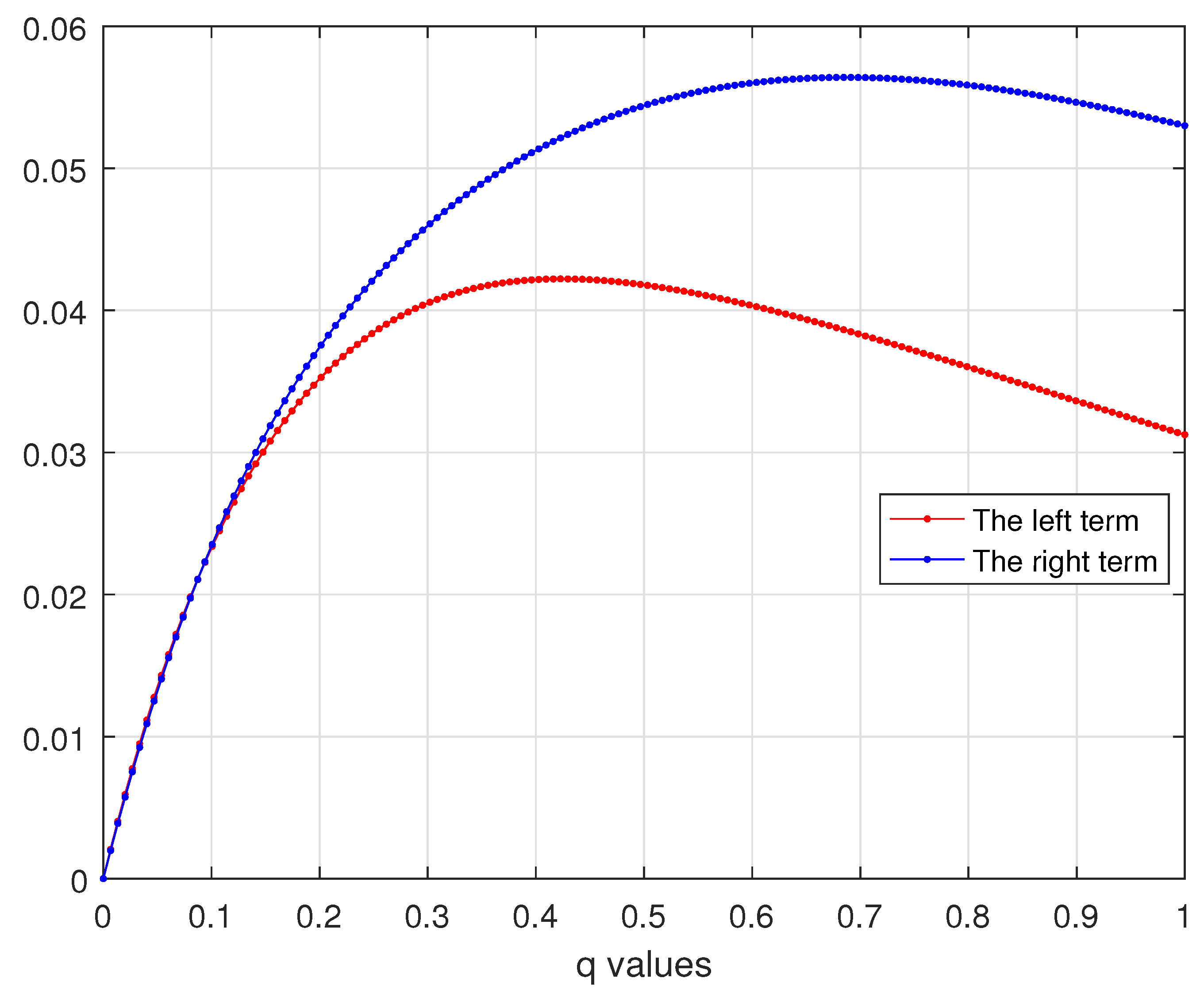
27 64 27 32 [ 2 ] q + 9 16 [ 3 ] q 1 8 [ 4 ] q 1 + 3 q 3 64 [ 2 ] q 3 q 3 4 [ 2 ] q ( 16 + 14 q 4 q 2 2 q 3 4 2 q 3 3 q 9 4 [ 2 ] q 3 [ 4 ] q 1 [ 2 ] q 3 [ 3 ] q 1 [ 2 ] q 2 [ 4 ] q 7 + 5 q 4 q 2 2 q 3 4 ) + 1 4 [ 2 ] q ( q + q 2 q 3 16 + 14 q 4 q 2 2 q 3 4 2 q 3 3 q 9 2 q + 4 q 2 + q 3 q 4 q 5 4 [ 2 ] q 3 [ 3 ] q [ 4 ] q q q 2 + 2 q 3 + 3 q 4 + 2 q 5 q 6 q 7 7 + 5 q 4 q 2 2 q 3 4 [ 2 ] q 4 [ 3 ] q [ 4 ] q ) .
The correctness of inequality (20) is verified in Figure 1.
Remark 3.
Putting  a 1 = ξ 1  and  b 1 = ξ 2  and taking limit  q 1  in Theorem 3, we have
1 ξ 2 ξ 1 ξ 1 ξ 2 f λ d λ f ξ 1 + ξ 2 2 ξ 2 ξ 1 2 48 f ξ 1 + f ξ 2 ,
proven in [34] [Theorem 3].
Remark 4.
Substituting  a 1 = ξ 1  and  b 1 = ξ 2  in Theorem 3, we have the results proven in [33] [Theorem 3].
Theorem 4.
Under the assumptions of Lemma 3, if  a 1 + b 1 ξ 1 D q 2 f 1 1 > 1 , is a convex function on  ξ 1 , ξ 2 , then we have
1 ξ 2 ξ 1 a 1 + b 1 ξ 2 a 1 + b 1 ξ 1 f ( λ ) a + b 1 ξ 1 d q λ f a 1 + b 1 ξ 2 + q ξ 1 [ 2 ] q q 3 ξ 2 ξ 1 2 2 q 3 + 1 2 2 2 + 1 q 1 2 ( a 1 + b 1 ξ 1 D q 2 f a 1 1 + a 1 + b 1 ξ 1 D q 2 f b 1 1 2 q a 1 + b 1 ξ 1 D q 2 f ξ 2 1 2 q 3 q 2 + 2 q a 1 + b 1 ξ 1 D q 2 f ξ 1 1 2 q 3 ) 1 1 + ξ 2 ξ 1 2 2 q φ ( q , 2 ) 1 2 × ( q a 1 + b 1 ξ 1 D q 2 f a 1 1 + a 1 + b 1 ξ 1 D q 2 f b 1 1 2 q [ 2 ] q 3 1 a 1 + b 1 ξ 1 D q 2 f ξ 1 1 2 q 3 q 2 + 2 q a 1 + b 1 ξ 1 D q 2 f ξ 2 1 2 q 3 ) 1 1 ,
where  1 1 + 1 2 = 1  and
φ ( q , 2 ) = 1 2 q 1 ( 1 q λ ) q 2 2 d q λ .
Proof. 
Employing the quantum Hölder’s inequality on Lemma 3, we have
1 ξ 2 ξ 1 a 1 + b 1 ξ 2 a 1 + b 1 ξ 1 f ( λ ) a + b 1 ξ 1 d q λ f a 1 + b 1 ξ 2 + q ξ 1 [ 2 ] q ξ 2 ξ 1 2 2 q q 3 0 1 2 q λ 2 2 d q λ 1 2 0 1 2 q a 1 + b 1 ξ 1 D q 2 f a 1 + b 1 λ ξ 2 + 1 λ ξ 1 1 d q λ 1 1 + ξ 2 ξ 1 2 2 q 1 2 q 1 ( 1 q λ ) q 2 2 d q λ 1 2 1 2 q 1 a 1 + b 1 ξ 1 D q 2 f a 1 + b 1 λ ξ 2 + 1 λ ξ 1 1 d q λ 1 1 .
Since  a 1 + b 1 ξ 1 D q 2 f 1  is convex on  ξ 1 , ξ 2 , we have
a 1 + b 1 ξ 1 D q 2 f a 1 + b 1 ( λ ξ 2 + 1 λ ξ 1 ) 1 a 1 + b 1 ξ 1 D q 2 f a 1 1 + a 1 + b 1 ξ 1 D q 2 f b 1 1 λ a 1 + b 1 ξ 1 D q 2 f ξ 2 1 1 λ a 1 + b 1 ξ 1 D q 2 f ξ 1 1 .
By Lemma 3, we have
1 ξ 2 ξ 1 a 1 + b 1 ξ 2 a 1 + b 1 ξ 1 f ( λ ) a + b 1 ξ 1 d q λ f a 1 + b 1 ξ 2 + q ξ 1 [ 2 ] q ξ 2 ξ 1 2 2 q q 3 1 2 q 2 2 + 1 2 2 + 1 q 1 2 ( 0 1 2 q ( a 1 + b 1 ξ 1 D q 2 f a 1 1 + a 1 + b 1 ξ 1 D q 2 f b 1 1 λ a 1 + b 1 ξ 1 D q 2 f ξ 2 1 1 λ a 1 + b 1 ξ 1 D q 2 f ξ 1 1 ) d q λ ) 1 1 + ξ 2 ξ 1 2 2 q φ ( q , 2 ) 1 2 ( 1 2 q 1 ( a 1 + b 1 ξ 1 D q 2 f a 1 1 + a 1 + b 1 ξ 1 D q 2 f b 1 1 λ a 1 + b 1 ξ 1 D q 2 f ξ 2 1 1 λ a 1 + b 1 ξ 1 D q 2 f ξ 1 1 ) d q λ ) 1 1 = q 3 ξ 2 ξ 1 2 2 q 2 q 2 2 + 1 2 2 2 + 1 q 1 2 ( a 1 + b 1 ξ 1 D q 2 f a 1 1 + a 1 + b 1 ξ 1 D q 2 f b 1 1 2 q a 1 + b 1 ξ 1 D q 2 f ξ 2 1 2 q 3 q 2 + 2 q a 1 + b 1 ξ 1 D q 2 f ξ 1 1 2 q 3 ) 1 1 + ξ 2 ξ 1 2 2 q φ ( q , 2 ) 1 2 × ( q a 1 + b 1 ξ 1 D q 2 f a 1 1 + a 1 + b 1 ξ 1 D q 2 f b 1 1 2 q [ 2 ] q 3 1 a 1 + b 1 ξ 1 D q 2 f ξ 1 1 2 q 3 q 2 + 2 q a 1 + b 1 ξ 1 D q 2 f ξ 2 1 2 q 3 ) 1 1 .
Remark 5.
Putting  a 1 = ξ 1  and  b 1 = ξ 2  and taking limit  q 1  in Theorem 4, we have the following result proven in [35] [Theorem 3 ]:
1 ξ 2 ξ 1 ξ 1 ξ 2 f λ d λ f ξ 1 + ξ 2 2 ξ 2 ξ 1 2 2 4 + 2 1 2 2 + 1 1 2 3 f ξ 1 1 + f ξ 2 1 1 1 + f ξ 1 1 + 3 f ξ 2 1 1 1 .
Remark 6.
Selecting  a 1 = ξ 1  and  b 1 = ξ 2  in Theorem 4 leads to the result given in [33] [Theorem 4].
Theorem 5.
Taking into account the considerations of Lemma 3, if  a 1 + b 1 ξ 1 D q 2 f 1 1 1 , and is convex on  ξ 1 , ξ 2 , then we have the inequality
1 ξ 2 ξ 1 a 1 + b 1 ξ 2 a 1 + b 1 ξ 1 f ( λ ) a + b 1 ξ 1 d q λ f a 1 + b 1 ξ 2 + q ξ 1 [ 2 ] q q 3 ξ 2 ξ 1 2 2 q 4 3 1 3 q 1 1 1 ( a + b 1 ξ 1 D q 2 f a 1 + a 1 + b 1 ξ 1 D q 2 f b 1 1 2 q 3 3 q a 1 + b 1 ξ 1 D q 2 f ξ 2 1 2 q 4 4 q 1 2 q 3 3 q 1 2 q 4 4 q q a 1 + b 1 ξ 1 D q 2 f ξ 1 1 ) 1 1 + q + q 2 q 3 1 1 1 ξ 2 ξ 1 2 2 q 4 3 1 3 q 1 1 1 ( q + q 2 q 3 2 q 3 3 q a 1 + b 1 ξ 1 D q 2 f a 1 1 + a 1 + b 1 ξ 1 D q 2 f b 1 1 2 q + 4 q 2 + q 3 q 4 q 5 2 q 4 3 q 4 q a + b 1 ξ 1 D q 2 f ξ 2 1 q q 2 + 2 q 3 + 3 q 4 + 2 q 5 q 6 q 7 2 q 4 3 q 4 q a 1 + b 1 ξ 1 D q 2 f ξ 1 1 ) 1 1 .
Proof. 
Practicing the power-mean inequality on Lemma 3 along with the convexity of  a 1 + b 1 ξ 1 D q 2 f 1 , we have
1 ξ 2 ξ 1 a 1 + b 1 ξ 2 a 1 + b 1 ξ 1 f ( λ ) a + b 1 ξ 1 d q λ f a 1 + b 1 ξ 2 + q ξ 1 [ 2 ] q ξ 2 ξ 1 2 2 q q 3 0 1 2 q λ 2 d q λ 1 1 1 0 1 2 q λ 2 a 1 + b 1 ξ 1 D q 2 f a 1 + b 1 λ ξ 2 1 λ ξ 1 1 d q λ 1 1 + ξ 2 ξ 1 2 2 q 1 2 q 1 ( 1 q λ ) q 2 d q λ 1 1 1 1 2 q 1 ( 1 q λ ) q 2 a 1 + b 1 ξ 1 D q 2 f a 1 + b 1 λ ξ 2 1 λ ξ 1 1 d q λ 1 1 ξ 2 ξ 1 2 2 q q 3 2 q 3 3 1 3 q 1 1 1 ( a 1 + b 1 ξ 1 D q 2 f a 1 1 + a 1 + b 1 ξ 1 D q 2 f b 1 1 0 1 2 q λ 2 d q λ a 1 + b 1 ξ 1 D q 2 f ξ 2 1 0 1 2 q λ 3 d q λ a 1 + b 1 ξ 1 D q 2 f ξ 1 1 0 1 2 q λ 2 λ 3 d q λ ) 1 1 + ξ 2 ξ 1 2 2 q ( 1 1 2 q ) q 3 1 1 1 3 q 1 1 1 ( a 1 + b 1 ξ 1 D q 2 f a 1 1 + a 1 + b 1 ξ 1 D q 2 f b 1 1 1 2 q 1 ( 1 q λ ) q 2 d q λ a 1 + b 1 ξ 1 D q 2 f ξ 2 1 1 2 q 1 λ ( 1 q λ ) q 2 d q λ a 1 + b 1 ξ 1 D q 2 f ξ 1 1 1 2 q 1 1 λ ( 1 q λ ) q 2 d q λ ) 1 1 = q 3 ξ 2 ξ 1 2 2 q 4 3 1 3 q 1 1 1 ( a + b 1 ξ 1 D q 2 f a 1 1 + a 1 + b 1 ξ 1 D q 2 f b 1 1 2 q 3 3 q a 1 + b 1 ξ 1 D q 2 f ξ 2 1 2 q 4 4 q 1 2 q 3 3 q 1 2 q 4 4 q q a 1 + b 1 ξ 1 D q 2 f ξ 1 1 ) 1 1 + q + q 2 q 3 1 1 1 ξ 2 ξ 1 2 2 q 4 3 1 3 q 1 1 1 ( q + q 2 q 3 2 q 3 3 q a 1 + b 1 ξ 1 D q 2 f a 1 1 + a 1 + b 1 ξ 1 D q 2 f b 1 1 2 q + 4 q 2 + q 3 q 4 q 5 2 q 4 3 q 4 q a + b 1 ξ 1 D q 2 f ξ 2 1 q q 2 + 2 q 3 + 3 q 4 + 2 q 5 q 6 q 7 2 q 4 3 q 4 q a 1 + b 1 ξ 1 D q 2 f ξ 1 1 ) 1 1 .
This completes the proof. □
Example 2.
Consider the same function  f  defined in Example 1. By  1 = 2 ,  the function
a 1 + b 1 ξ 1 D q 2 f λ 2 = ( [ 4 ] q + q [ 2 ] q ) λ + 3 4 2 + q ( 1 q 2 ) 2 .
is convex on  0 , 1 .  Thus, using Theorem 5 along with Definition 4, the L.H.S. of the inequality (22) is similar to (19).
On the other hand, we can calculate the R.H.S. of the inequality (22) as follows:
q 3 ξ 2 ξ 1 2 2 q 4 3 1 3 q 1 1 1 ( a + b 1 ξ 1 D q 2 f a 1 + a 1 + b 1 ξ 1 D q 2 f b 1 1 2 q 3 3 q a 1 + b 1 ξ 1 D q 2 f ξ 2 1 2 q 4 4 q 1 2 q 3 3 q 1 2 q 4 4 q q a 1 + b 1 ξ 1 D q 2 f ξ 1 1 ) 1 1 + q + q 2 q 3 1 1 1 ξ 2 ξ 1 2 2 q 4 3 1 3 q 1 1 1 ( q + q 2 q 3 2 q 3 3 q a 1 + b 1 ξ 1 D q 2 f a 1 1 + a 1 + b 1 ξ 1 D q 2 f b 1 1 2 q + 4 q 2 + q 3 q 4 q 5 2 q 4 3 q 4 q a + b 1 ξ 1 D q 2 f ξ 2 1 q q 2 + 2 q 3 + 3 q 4 + 2 q 5 q 6 q 7 2 q 4 3 q 4 q a 1 + b 1 ξ 1 D q 2 f ξ 1 1 ) 1 1 . = q 3 4 2 q 5 3 q 1 2 ( 6 + 3 q 6 q 2 3 q 3 2 + 10 + 11 q + 2 q 2 + q 3 2 16 2 q 3 3 q 81 16 2 q 2 4 q 1 2 q 3 3 q 1 2 q 4 4 q q 7 + 5 q 4 q 2 2 q 3 2 16 ) 1 1 + q + q 2 q 3 1 2 ξ 2 ξ 1 2 4 2 q 5 3 q 1 2 × ( q + q 2 q 3 16 2 q 3 3 q 6 + 3 q 6 q 2 3 q 3 2 + 10 + 11 q + 2 q 2 + q 3 2 81 2 q + 4 q 2 + q 3 q 4 q 5 16 2 q 2 3 q 4 q q q 2 + 2 q 3 + 3 q 4 + 2 q 5 q 6 q 7 7 + 5 q 4 q 2 2 q 3 2 16 2 q 4 3 q 4 q ) 1 1 .
Then, by inequality (22), we have
27 64 27 32 [ 2 ] q + 9 16 [ 3 ] q 1 8 [ 4 ] q 1 + 3 q 3 64 [ 2 ] q 3 q 3 4 2 q 5 3 q 1 2 ( 6 + 3 q 6 q 2 3 q 3 2 + 10 + 11 q + 2 q 2 + q 3 2 16 2 q 3 3 q 81 16 2 q 2 4 q 1 2 q 3 3 q 1 2 q 4 4 q q 7 + 5 q 4 q 2 2 q 3 2 16 ) 1 1 + q + q 2 q 3 1 2 ξ 2 ξ 1 2 4 2 q 5 3 q 1 2 × ( q + q 2 q 3 16 2 q 3 3 q 6 + 3 q 6 q 2 3 q 3 2 + 10 + 11 q + 2 q 2 + q 3 2 81 2 q + 4 q 2 + q 3 q 4 q 5 16 2 q 2 3 q 4 q q q 2 + 2 q 3 + 3 q 4 + 2 q 5 q 6 q 7 7 + 5 q 4 q 2 2 q 3 2 16 2 q 4 3 q 4 q ) 1 1 .
One can see the validity of inequality (24) in Figure 2.
Remark 7.
Choosing the limit as  q 1 a 1 = ξ 1 , and  b 1 = ξ 2  in Theorem 5, we attain
1 ξ 2 ξ 1 ξ 1 ξ 2 f λ d λ f ξ 1 + ξ 2 2 ξ 2 ξ 1 2 3 2 4 + 3 1 5 f ξ 1 1 + 3 f ξ 2 1 1 1 + 3 f ξ 1 1 + 5 f ξ 2 1 1 1
proven in [35] [Theorem 4].
Remark 8.
Substituting  a 1 = ξ 1  and  b 1 = ξ 2  in Theorem 5, we recapture the result mentioned in [33] [Theorem 5].

4. Concluding Remarks

To summarize, we obtained new quantum estimates of Mercer midpoint inequalities for convex functions, which represent a significant generalization of previously published related results. Our findings demonstrate the potential for further research in this area, particularly in exploring the use of different types of convexity to derive new bounds. It is necessary to state that our primary results can be reduced to classical calculus by choosing  q 1 a 1 = ξ 1 , and  b 1 = ξ 2 . We feel that this opens up a fascinating and novel research direction for scholars to explore, where analogous inequalities can be obtained by using different types of convexity.

Author Contributions

Conceptualization, S.I.B.; funding acquisition, S.I.B.; investigation, M.U. and H.B.; methodology, M.U.; validation, H.B.; visualization, S.I.B. and H.B.; writing—original draft, S.I.B. and M.U.; writing—review and editing, H.B. All authors have read and agreed to the published version of the manuscript.

Funding

This research received no external funding.

Institutional Review Board Statement

Not applicable.

Informed Consent Statement

Not applicable.

Data Availability Statement

Not applicable.

Conflicts of Interest

The authors declare no conflict of interest.

References

  1. Mitrinović, D.S.; Pexcxarixcx, J.E.; Fink, A.M. Classical and New Inequalities in Analysis. In Mathematics and Its Applications (East and European Series); Kluwer Academic Publishers Group: Dordecht, The Netherlands, 1993. [Google Scholar]
  2. Liu, L.; Wang, J.; Zhang, L.; Zhang, S. Multi-AUV Dynamic Maneuver Countermeasure Algorithm Based on Interval Information Game and Fractional-Order DE. Fractal Fract. 2022, 6, 235. [Google Scholar] [CrossRef]
  3. He, Y.; Zhang, L.; Tong, M.S. Microwave Imaging of3D Dielectric-Magnetic Penetrable Objects Based on Integral Equation Method. IEEE Trans. Antennas Propag. 2023. [Google Scholar] [CrossRef]
  4. Wu, Y.; Yang, X. The Impact of Contract Enforcement Efficiency on Debt Maturity Structure Using Mathematical Derivation and Comparative Static Analysis. J. Comput. Methods Sci. Eng. 2022, 22, 97–108. [Google Scholar] [CrossRef]
  5. Shen, Q.; Yang, Z. Applied mathematical analysis of organizational learning culture and new media technology acceptance based on regression statistical software and a moderated mediator model. J. Comput. Methods Sci. Eng. 2021, 21, 1825–1842. [Google Scholar] [CrossRef]
  6. Mehmood, N.; Butt, S.I.; Pećarixcx, D.; Pexcxarixcx, J. Generalizations of Cyclic Refinements of Jensen’s Inequality by Lidstone’s Polynomial with Applications in Information Theory. J. Math. Inequal. 2019, 14, 249–271. [Google Scholar] [CrossRef]
  7. Khan, S.; Khan, M.A.; Butt, S.I.; Chu, Y.M. A New Bound for the Jensen Gap Pertaining Twice Differentiable Functions with Applications. Adv. Differ. Equ. 2020, 2020, 333. [Google Scholar] [CrossRef]
  8. Mercer, A.M. A Variant of Jensens Inequality. J. Inequalities Pure Appl. Math. 2003, 4, 73. [Google Scholar]
  9. Kian, M.; Moslehian, M.S. Refinements of the Operator Jensen–Mercer Inequality. Electron. J. Linear Algebra 2013, 26, 742–753. [Google Scholar] [CrossRef]
  10. Anjidani, E. Jensen–Mercer Operator Inequalities Involving Superquadratic Functions. Mediterr. J. Math. 2018, 15, 31. [Google Scholar] [CrossRef]
  11. Moradi, H.R.; Furuichi, S. Improvement and Generalization of Some Jensen–Mercer–Type Inequalities. J. Math. Inequalities 2020, 14, 377–383. [Google Scholar] [CrossRef]
  12. Khan, M.A.; Husain, Z.; Chu, Y.M. New Estimates for Csiszar Divergence and Zipf-Mandelbrot Entropy via Jensen-Mercer’s Inequality. Complexity 2020, 2020, 8928691. [Google Scholar]
  13. Ernst, T. The History Of q-Calculus and New Method; Department of Mathematics, Uppsala University: Uppsala, Sweden, 2000. [Google Scholar]
  14. Gauchman, H. Integral Inequalities in q-Calculus. Comput. Math. Appl. 2004, 47, 281–300. [Google Scholar] [CrossRef]
  15. Jackson, F.H. On a q-Definite Integrals. Q. J. Pure Appl. Math. 1910, 41, 193–203. [Google Scholar]
  16. Kac, V.; Cheung, P. Quantum Calculus, Universitext; Springer: New York, NY, USA, 2002. [Google Scholar]
  17. Rajkovic, P.M.; Stankovic, M.S.; Marinkovic, S.D. The Zeros of Polynomials Orthogonal with Respect to q-Integral on Several Intervals in the Complex Plane. In Proceedings of the Fifth International Conference on Geometry, Integrability and Quantization, Varna, Bulgaria, 5–12 June 2003. [Google Scholar]
  18. Alp, N.; Sarikaya, M.Z.; Kunt, M.; Iscan, I. q-Hermite Hadamard Inequalities and Quantum Estimates for Midpoint Type Inequalities Via Convex and Quasi-Convex Functions. J. King Saud Univ. Sci. 2018, 30, 193–203. [Google Scholar] [CrossRef]
  19. Bermudo, S.; Kórus, P.; Valdés, J.N. On q-Hermite–Hadamard Inequalities for General Convex Functions. Acta Math. Hung. 2020, 162, 364–374. [Google Scholar] [CrossRef]
  20. Alp, N.; Budak, H.; Erden, S.; Sarikaya, M.Z. New Bounds q-Midpoint Type Inequalities for Twice q-Differentiable Convex Functions on Quantum Calculus. Soft Comput. 2022, 26, 10321–10329. [Google Scholar] [CrossRef]
  21. Tariboon, J.; Ntouyas, S.K. Quantum integral inequalities on finite intervals. J. Inequal. Appl. 2014, 2014, 121. [Google Scholar] [CrossRef]
  22. Mohammed, P.O. Some integral inequalities of fractional quantum type. Malaya J. Mat. 2016, 4, 93–99. [Google Scholar]
  23. Noor, M.A.; Noor, K.I.; Awan, M.U. Some quantum estimates for Hermite Hadamard inequalities. Appl. Math. Comput. 2015, 251, 675–679. [Google Scholar] [CrossRef]
  24. Xu, P.; Butt, S.I.; Ain, Q.U.; Budak, H. New Estimates for Hermite-Hadamard Inequality in Quantum Calculus via (α, m)-Convexity. Symmetry 2022, 14, 1394. [Google Scholar] [CrossRef]
  25. Alqudah, M.A.; Kashuri, A.; Mohammed, P.O.; Abdeljawad, T.; Raees, M.; Anwar, M.; Hamed, Y.S. Hermite-Hadamard Integral Inequalities on Co-ordinated Convex Functions in Quantum Calculus. Adv. Differ. Equ. 2021, 2021, 264. [Google Scholar] [CrossRef]
  26. Rashid, S.; Butt, S.I.; Kanwal, S.; Ahmad, H.; Wang, M.K. Quantum integral inequalities with respect to Raina’s function via coordinated generalized-convex functions with applications. J. Funct. Spaces. 2021, 2021, 6631474. [Google Scholar] [CrossRef]
  27. Ali, M.A.; Alp, N.; Budak, H.; Chu, Y.; Zhang, Z. On Some New Quantum Midpoint Type Inequalities for Twice Quantum Differentiable Convex Functions. Open Math. 2021, 19, 427–439. [Google Scholar] [CrossRef]
  28. Butt, S.I.; Budak, H.; Nonlaopon, K. New Variants of Quantum Midpoint-Type Inequalities. Symmetry 2022, 14, 2599. [Google Scholar] [CrossRef]
  29. Budak, H.; Kara, H. On Quantum Hermite-Jensen-Mercer Inequalities. Miskolc Math. Notes, 2020; accepted. [Google Scholar]
  30. Mosin, B.B.; Saba, M.; Javed, M.Z.; Awan, M.U.; Budak, H.; Nonlaopon, K. A Quantum Calculus View of Hermite-Hadamard-Jensen-Mercer Inequalities with Applications. Symmetry 2022, 14, 1246. [Google Scholar] [CrossRef]
  31. Bohner, M.; Budak, H.; Kara, H. Post-Quantum Hermite-Jensen-Mercer Inequalities. Rocky Mt. J. Math. 2022; in press. [Google Scholar]
  32. Butt, S.I.; Budak, H.; Nonlaopon, K. New Quantum Mercer Estimates of Simpson-Newton like Inequalities via Convexity. Symmetry 2022, 14, 1935. [Google Scholar] [CrossRef]
  33. Siricharuanun, P.; Erden, S.; Ali, M.A.; Budak, H.; Chasreechai, S.; Sitthiwirattham, T. Some New Simpson’s and Newton’s Formulas Type Inequalities for Convex Functions in Quantum Calculus. Mathematics 2021, 9, 1992. [Google Scholar] [CrossRef]
  34. Sarikaya, M.Z.; Saglam, A.; Yildirim, H. New Inequalities of Hermite-Hadamard Type for Functions Whose Second Derivatives Absolute Values are Convex and Quasi-convex. Int. J. Open Probl. Comput. Sci. Math. 2012, 5. [Google Scholar] [CrossRef]
  35. Noor, M.A.; Awan, M.U. Some integral inequalities for two kinds of convexities via fractional integrals. Transylv. J. Math. Mech. 2013, 5, 129–136. [Google Scholar]
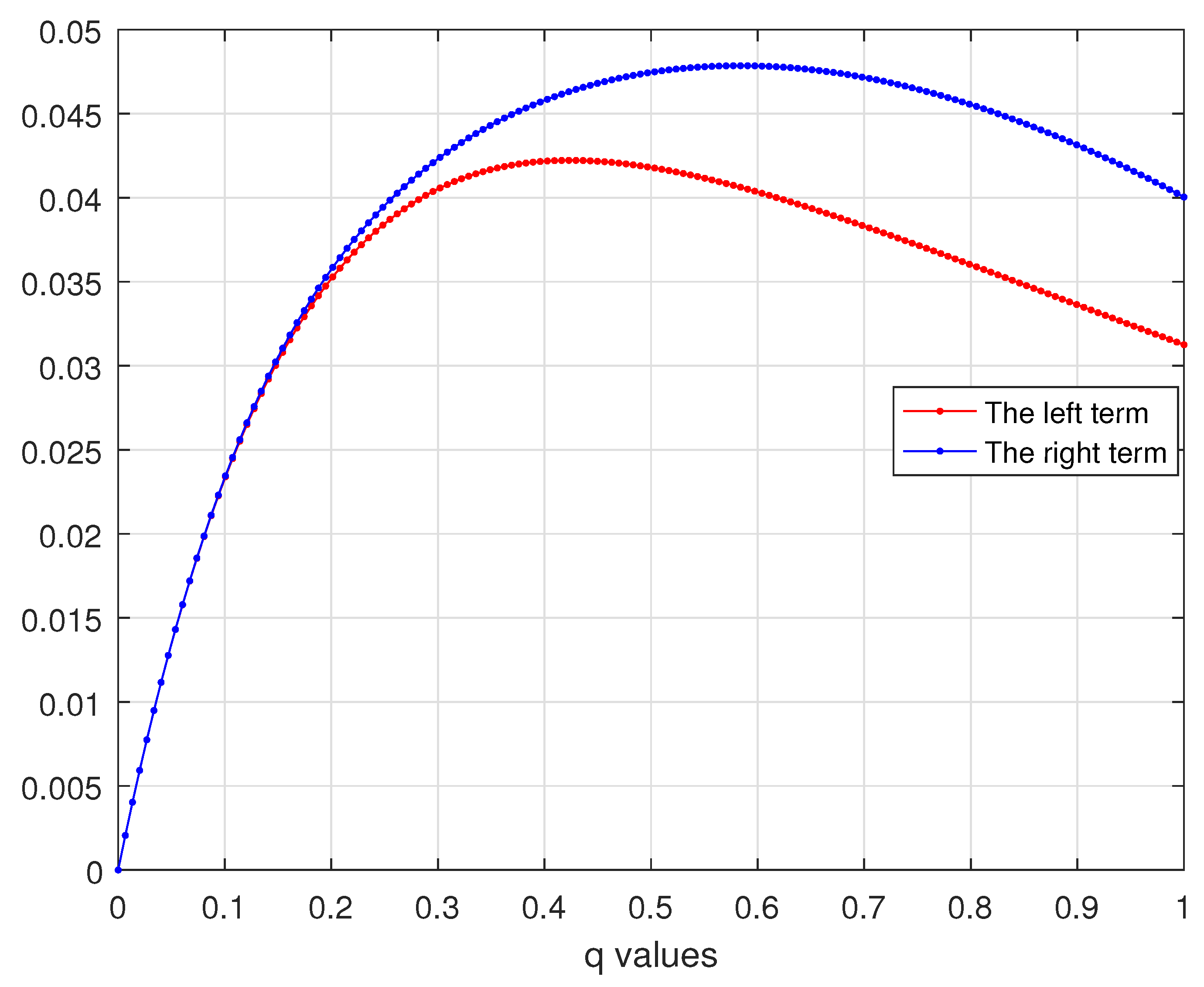
Figure 1. An example of inequality (12).
Symmetry 15 01038 g001
Figure 2. An example of inequality (22).
Symmetry 15 01038 g002
Disclaimer/Publisher’s Note: The statements, opinions and data contained in all publications are solely those of the individual author(s) and contributor(s) and not of MDPI and/or the editor(s). MDPI and/or the editor(s) disclaim responsibility for any injury to people or property resulting from any ideas, methods, instructions or products referred to in the content.