Abstract
Several non-functional objects are orbiting around the Earth and they are called space debris. In this work, we investigate the process of space debris mitigation from the GEO region using a solar sail. The acceleration induced by the solar radiation pressure (SRP) is the most relevant perturbation for objects in orbit around the Earth with a high area-to-mass ratio (). We consider the single-averaged SRP model with the Sun in an elliptical and inclined orbit. In addition to the SRP effect, the orbital evolution of space debris is analyzed considering the perturbations due to the Earth’s flattening and third-body perturbations in the dynamical system. The idea is to use the solar sail as a propulsion system using the Sun itself as a clean and abundant energy source so that it can remove space debris from the geostationary orbit and also contribute to the sustainability of space exploration. Using averaged dynamical maps as a tool, the numerical simulations show that the solar sail contributes strongly to exciting the eccentricity of the space debris, causing its reentry into Earth’s atmosphere. To perform the numerical simulations, we consider data from real space debris. We also show that the solar sail can be used to remove space debris for a graveyard orbit. In this way, the solar sail can work as a clean and sustainable space-debris-removal mechanism. Finally, we show that the convenient choice of the argument of perigee and the longitude of the ascending node might contribute to amplify the growth of eccentricity. It is also shown that solar radiation pressure destroys the symmetry of the orbits that can be observed in keplerian orbits, so all the orbits will be asymmetric when considering the presence of this force.
1. Introduction
According to the Mitigation Guidelines of the Inter-Agency Space Debris Coordination Committee (IADC), which is a governmental forum with the goal of coordinating activities related to natural and man-made space debris. Artificial space debris is “all man made objects including fragments and elements thereof, in Earth orbit or re-entering the atmosphere, that are non functional” [1,2,3]. The amount of space debris has increased considerably in recent decades. These objects present risks for users of the space environment when one thinks about the integrity of operational spacecraft and the contamination of orbital regions around the Earth. They can damage active satellites orbiting the Earth, or they can collide with other debris, generating a cloud of even smaller debris [4]. In addition, a possible uncontrolled fall of these objects might create a great harm to society.
The issue of space debris dates back to the 1970s. Donald Kessler and Burton Cour-Palai stated in their 1978 article Collision Frequency of Artificial Satellites: The Creation of a Debris Belt that it was conceivable that a significant number of satellite fragments already existed at that time around the Earth [5]. According to these authors, fragments that are not covered by radar probably have their origin in tests of “killer satellites” and due to accidental explosions of rocket engines (launch vehicles). In 1979, Czech astronomer Lubos Perek presented an article called Outer Space Activities versus Outer Space, which recommends several space-debris-mitigation techniques [2,6]. At the time, Perek said that preventing all collision events is impossible, so minimizing their effects, while costly, is more cost-effective compared to repairing the damage that does occur. In his work, Perek suggests ideas such as reducing the amount of debris produced during launch and in-orbit operations, de-orbiting inactive satellites, redirecting inactive satellites to discard orbits, and using orbits that do not cross certain specific areas/regions of the space around the Earth [7]. In 1991, Donald Kessler analyzed the problem of collisions between orbital objects in an article entitled Collisional Cascading: The Limits of Population Growth in Low-Earth Orbits. In this article, the author points to the problems involved with the fast-growing numbers of space debris, initially formed by collisions between objects and, finally, increased by collisions between the fragments [2,8]. The collisional cascade phenomenon was later, and since then, known as Kessler’s Syndrome and cannot be stopped in its advanced stage. Several other studies [9,10,11,12] have been carried out with the interest in finding a solution to mitigate the risks involved with the presence of space debris around our planet.
The IADC, in its Mitigation Guidelines, further establishes that any activity developed in space must be carried out recognizing as unique—in the sense of a finite resource—certain regions of the space surrounding planet Earth. The idea is to guarantee its safe and sustainable future use. In this sense, these regions must be protected from the generation of space debris [1]. One of these regions, called Region B, or the geosynchronous region, according to the IADC, is a spherical shell segment defined by a range of altitudes with respect to the geostationary altitude (35,786 km). The limits of this range are a lower margin of 200 km and an upper margin of 200 km with respect to the geostationary altitude. This region is also inside an interval of 15 degrees of latitude centered on the celestial equatorial plane, in which the geostationary orbit (GEO) is located [1]. By definition, GEO and the torus-shaped region that surrounds it are unique and are of great importance for space activities due to the favorable/advantageous orbital characteristics that the satellites assume, especially for the telecommunications area, when placed at such altitudes. Given the importance of this orbital region, the mitigation capacity of its inoperative objects becomes extremely important in order to avoid, for various reasons, its contamination by space debris. In fact, in 1978, the first event of debris generation in the GEO regime occurred [2,13]. At that time, there was a fragmentation of the Russian-Soviet artificial satellite Ekran 2, with a nominal orbital inclination of , according to reports, due to battery problems [14]. In this work, as a matter of nomenclature, the space debris whose nominal orbits (ongoing) evolve inside this torus-shaped region, whose center is the GEO, are classified as debris in a geostationary orbital regime (GEO orbital regime) or GEO region. In this context, this work aims to analyze the possibility of removing space debris from the GEO region in order to promote its disposal in a graveyard orbit, thus allowing the safe and sustainable use of this important orbital regime. In order to fulfill this objective, the use of some device that excites the nominal orbit of the object with the purpose of its orbital relocation is suggested. The device considered in this work is a solar sail.
Regarding its structure, a solar sail is made of a large glowing membrane composed of a thin reflective film that covers the structure of the spacecraft [15]. From the point of view of devices to be boarded in a space vehicle, a solar sail must meet the requirements of being a large, flat, light, and reflective surface that can propel a space vehicle without the use of propellants [16]. Based on this definition, as a proposal for mitigating space debris in a GEO region, this work proposes a practice of orbital debris relocation aimed at removing these objects from such a regime by disposing of them in a graveyard orbit. For this, a solar sail can be used as a device on board space vehicles whose mission takes place in the GEO regime. It is suggested that, at the end of the life cycle of these vehicles, the solar sail can be activated, allowing, through the disturbing effect of the solar radiation pressure (SRP), the eccentricity and peak altitude of the vehicle to be increased, moving it from the GEO regime to an altitude above this region. The use of the solar sail is justified, because such a device is a propulsion medium not limited to the dependence of a finite amount of reaction mass (propellant) and that gives a continuous acceleration, whose limit is the lifetime of the sail film. The solar sail gains impulse from an environmental source, the photons [15] emitted by the Sun, which are abundant and constitute a source of clean energy. In fact, according to studies available in the literature, an object with a small area-to-mass ratio that is in a GEO region can remain there for hundreds of years [11]. Therefore, the solar sail will enable, by increasing the area-to-mass ratio of the space vehicle (debris) using the model proposed here, the preventive mitigation of a disused space object through its disposal in a graveyard orbit. As a discard altitude criterion, a margin of km above the GEO altitude ( km) is considered. Thus, when activating the solar sail, using the model proposed in this work, the effect of the SRP is expected to move the satellite (debris) coupled to the sail until an altitude of is reached. Then, it is suggested that the sail should be closed or uncoupled from the debris, such that this object will start to occupy a higher disposal orbit that is distant enough from the GEO region.
Despite the fact that the SRP is the strongest perturbation when the object has a high area-to-mass ratio [10,17], the presence of other forces in the space environment is not negligible. Thus, the use of a solar sail combined with the natural environmental disturbances is considered. For instance, in [17], a semi-analytical theory is presented considering the effects of the direct SRP and the atmospheric drag in the orbit of a spacecraft around the Earth. The equations obtained, when disregarding the SRP, eliminate the spurious Poisson terms from the theory of Brouwer and Hori [18,19]. In the case of this work, the mathematical model considers only the main perturbing forces acting on the space debris in a GEO regime, such as the forces associated with the direct solar radiation pressure (denoted already as SRP), the third-body perturbations from the Sun and Moon (TBP), and the flattening of the Earth, expressed as the dominant term of its potential, namely the second-degree zonal harmonic coefficient . The goal is to use the changes over the orbital eccentricity along with the increase in the perigee altitude of these objects until they reach the outside of the borders of the GEO region.
In the present study, we adopted averaged dynamics to study the orbital motion, since it has been successfully applied to several studies seeking a qualitative approach for the long-term dynamical evolution of a system (see, for instance, the applications of this type of dynamics presented in references [20,21,22,23,24,25]). In this study, a model for the SRP acceleration is used that can be associated with a potential, because it depends only on the radial position of the solar sail with respect to the Sun [15], which generates the photon emission. Such a consideration allows the disturbing potential associated to the SRP to be written in a series of polynomials of Legendre. In a recent work, Tresaco et al. [26] developed the SRP equation using the double-averaged model considering the Earth in an elliptical and inclined orbit around the Sun. It is assumed that the solar sail maintains an orientation perpendicular to the line of the Sun and the sail is located at a distance from the Sun such that the SRP model can be expressed by a potential function. Neglecting the effect of the Earth’s shadow, the system is Hamiltonian. Thus, the equations are developed using Legendre polynomial expansions up to the second order. In the double-averaged model, the first-order term of the expansion of the Legendre polynomial does not contain the terms of the orbital elements of the satellite (or debris), and therefore, when it is replaced in the Lagrange planetary equations, it does not affect its orbital elements. Thus, in [26] the first-order term is neglected and only the second-order term of the Legendre polynomial is used in the dynamical system. In [27], the authors remake the modeling presented in [26], but, in this case, it is taking into account the single-averaged model. With this approach, the first-order term of the expansion of the Legendre polynomial contains the terms of the orbital elements of the satellite (debris), and thus affect the orbital elements when it is substituted in the Lagrange planetary equations. The authors showed that the first-order SRP model is dominant compared to the second-order expansion term; that is, the first-order equation coming from the SRP is the main perturbation of the model and its effect is much greater than the term of second order. It is shown that the SRP acts strongly on the debris in the GEO region, allowing an increase in their eccentricity. This increase is proportional to the area/mass ratio of the debris.
Several authors have taken into account the solar radiation pressure models to explore the dynamics of artificial satellites, asteroids, and space debris; for example, see references [9,10,11,27,28,29,30,31,32,33,34,35,36] (and references therein). For the equation of the perturbing potential due to a third body, we use a single-averaged model [37] including the perturbations coming from the Sun and Moon and assuming that these perturbing bodies are moving in elliptical and inclined orbits. The equation of the disturbing potential due to the third body can be seen in Appendix B of reference [37]. It is important to mention that, in the present work, the effect of the shadow of the Earth is not included in the mathematical model, because, as presented in [32], it is not very important to the dynamics. Finally, as an analysis tool of the proposed model, averaged dynamical maps will be used, which have already been used in studies considering SRP [22,38] along with plots of the temporal behavior of some orbital elements of the space debris, such as its orbital eccentricity, to show that the solar sail contributes considerably to the orbital excitation of space debris in the GEO regime, promoting its relocation and disposal in a graveyard orbit or pushing the debris back into the atmosphere of the Earth. Finally, according to [36], the application of proper elements has been used to identify families of asteroids and more recently, they have been used in the context of space debris. The authors describe the dynamics of space debris considering the proper elements, taking into account a model that includes the gravitational attraction of the Earth, the influence of the Sun and Moon, and the solar radiation pressure. In general, we observed that when the SRP is taken into account the presence of perturbations destroys completely the symmetry of the orbits.
2. Mathematical Model
The physical model adopted for the forces considered in the dynamics used here takes into account the Earth’s flattening at the poles, the perturbations from the Sun and Moon, and the SRP. The equation of motion of the debris can be written as
where is the force due to the Earth’s gravitational field, the terms and are the resulting forces due to the third-body gravitational attractions of the Sun and Moon, respectively, and the term represents the acceleration generated by SRP. The term is given by , where is the direct acceleration due to the gravitational central force of the Earth and is the disturbing acceleration given by the Earth’s flattening at the poles. After several algebraic manipulations, Equation (1) can be defined as a function of the orbital elements of the space debris: a—semi-major axis, e—eccentricity, i—inclination, g—argument of perigee, h—longitude of the ascending node, and l—mean anomaly. In this work, we rewrite the equation of motion given by Equation (1) as a gradient of a potential and we present the disturbing potential as a function of the orbital elements. The algebraic development of the equations considered here is taken from references [27,37].
After convenient algebraic manipulations, the equation to represent the oblateness of the Earth (), using the single-averaged method, can be written as [27,37]
where is the equatorial radius of the Earth, n is the angular velocity of the satellite (debris) (mean motion, i.e., ), and is the Earth’s gravitational parameter. The term due to the irregular shape of the Earth () considered in the present work represents the second term of the gravity field of the Earth, which represents the flattening at the poles. The disturbing potential due to SRP () using a single-averaged model and assuming the Sun in elliptical and inclined orbits is written as [27]
where and are the mean motion and mean anomaly of the Sun, respectively. The orbital elements from the Sun are written with the index . The parameter is defined by
where . Here, is the Sun’s luminosity, c is the speed of light, and is the Sun’s gravitational parameter. For the Earth’s case, g/m[15]. The term is the sail-loading parameter (density of the area) and it is given by the spacecraft’s mass m (debris) divided by the area A of the sail. It is expressed in g/m. Note that the equations of the perturbing potentials due to the Sun and Moon ( and , respectively) will not be given explicitly here (we refer the reader to [37], where the authors consider the third body in an elliptical and inclined orbit—see Appendix B of reference [37]).
The last disturbing potential used in this present work is
Considering the perturbations previously commented, we replace Equation (5) into Lagrange’s planetary equations and numerically integrate the set of nonlinear differential equations to obtain the variations of the orbital elements of the space debris. After the numerical integrations, we show the results in the next section. The idea is to move the satellite (debris) into an orbit with an altitude higher than the GEO region, where artificial satellites for communications, military use, meteorology, and other applications are located. In addition, this region presents deactivated satellites, parts of satellites after their fragmentation, etc. To avoid the risk of these non-operational objects colliding with operational satellites, it is necessary to clean the GEO region. Thus, we propose to elevate the orbits of the space debris to a region above this protected GEO “ring”, which is commonly called a graveyard orbit, considering a solar sail such that the orbital perturbations included will help to amplify the growth of the eccentricity of the debris. As mentioned before and discussed in [27], the first-order SRP is the predominant perturbation due to the high ratio of the satellite (debris) after it is coupled to a solar sail. We also analyze the possibility of removing space debris from the GEO region by pushing it towards the Earth atmosphere. To perform this task, a large solar sail is used to increase the eccentricity of the debris such that it reaches the so-called reentry region.
3. Numerical Experiments with Real Debris Orbital Data
Now we show the results obtained from the numerical experiments. The data for the space debris used in the simulations is taken from the “stuffin.space” website, a platform that receives daily updates with orbital data from “Space-Track.org”. The orbital data of the debris considered in the dynamics for each result presented here is presented in the legend of each figure. The disturbing potential given by Equation (5) is replaced into the system of the Lagrange planetary equations. This system of equations is numerically integrated using Maple software. For the numerical integration of the dynamical system, we use Maple’s dsolve routine with the options “numeric” and “method = rkf45”, which represents an integration using the Runge–Kutta–Fehlberg method.
In the mentioned website, http://stuffin.space/ (accessed on 7 September 2022), we obtain the initial conditions of real debris, called BLOCK DM–SL–DEB (2019–095E), which we will call Case 1. Here, we investigate the mitigation process by removing the debris into a graveyard orbit. Thus, we consider raising the debris to a new orbit 1000 km above the geostationary ring. To perform this maneuver, we assume that we have a solar sail coupled to the satellite with different values of , namely m/kg and natural disturbances such as SRP, the flattening of Earth (), and the gravitational perturbation of the Moon and the Sun.
Figure 1a shows that the eccentricity increases proportionally to the increase in the ratio in a short period of time. That is, the greater the value of A/m, the greater the variation in the eccentricity of the debris in a short period of time. We see that, in less than one year, the eccentricity reaches a considerable variation for all cases analyzed for the values of A/m. Figure 1b shows the increase in inclination also for different values of . Note that the time to increase the variation of the inclination is much longer than the eccentricity case, but there is a large inclination variation anyway. This can be used to change the orbital plane of the debris. Note that we use zero for the argument of perigee and longitude of the ascending node, because the site does not provide the values of these orbital elements.
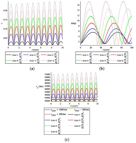
Figure 1.
Case 1. Payload object: BLOCK DM–SL–DEB (2019–095E). Initial conditions: km, , , , . Disturbing potential: . Period of integration: (a) 10 years; (b) 100 years; (c) 10 years.
Figure 1c shows the apogee position. The horizontal lines in yellow and red represent the protected GEO region. The black horizontal line represents the altitude of the chosen graveyard orbit, which in this case is 1000 km above (35,786 km). Note that, with just a solar sail with m/kg, the debris is directed to the desired orbit. However, note also that, if no other maneuvers are performed, the debris returns to its initial orbit. Then, when it reaches the desired altitude, a new maneuver must be performed so that the debris remains in the orbit 1000 km above the protected region. This maneuver, which must be performed when the debris reaches the desired altitude, is not the focus of this work. Here, our main objective is to choose the parameter for the debris to reach the desired altitude. Furthermore, another objective is to choose convenient values for the argument of perigee (g) and the longitude of the ascending node (h) that amplify the growth of the eccentricity. To verify the contributions of these orbital elements, we plotted dynamical (color) maps (see Figure 2a) varying the initial conditions for the argument of perigee and longitude of the ascending node from 0 to 360 degrees with steps of 5 degrees. In the color scale we show the amplitude of the eccentricity ().

Figure 2.
Case 1. Payload object: BLOCK DM–SL–DEB (2019–095E). Initial conditions: km, , . Parameters: and steps of , and steps of . Disturbing potential: . . Time of integration: 5 years, m/kg. (a) Color bar is given by ; (b) Color bar is the time to obtain the eccentricity in (a).
As shown in Figure 2a, the amplitude of the eccentricity depends on the initial values of . In this way, we can direct the debris to one of these values of that will help to amplify the orbital eccentricity of the debris. The redder colors show the peak amplitude of the eccentricity of the debris. Thus, besides choosing , the pair also contributes to direct the debris to a previously established graveyard orbit. Figure 2a was generated considering = 1 m/kg, that initially the debris is not disturbed enough to reach the graveyard orbit, as shown in Figure 1c. However, according to Figure 2a, some values of () help to amplify the eccentricity of the debris. That is, taking the perturbation was not enough to increase the initial value of the eccentricity for the values of () considered initially (see Figure 1c), but Figure 2a shows that there are some values of () that can amplify the eccentricity and so the debris can enter the bounded region for the graveyard orbit.
Note that Figure 2b shows the regions where the values of () contribute to amplifying the eccentricity, and the color scale shows the time for this eccentricity growth to occur. Thus, we can observe that, even with a solar sail with = 1 m/kg, the debris had its eccentricity increased, allowing the object to be directed to the graveyard orbit. Then, it is possible to say that, using a solar sail with a lower area-to-mass ratio, which contributes in technical terms to reduce costs, it is possible to perform the desired maneuver by directing the debris to a certain value of . Note that we used and as initial conditions in the simulations that generated Figure 1c but, as we can see in Figure 2a, this value contributes little to the growth of the eccentricity, highlighted in the blue color scale. However, for other initial values of these angles, a region with accentuated values of eccentricity is obtained, which contributes to the purpose of this work.
Case 2 takes into account the TITAN 3C TRANSTAGE DEB-1968-081H debris. The initial conditions can be seen by looking at the legend of Figure 3a. Comparing Figure 3a with Figure 1a, we can see that the eccentricity growth shown in Figure 3a is more pronounced than in the case of Figure 1a. We also see that the pattern remains the same, that is, increasing the eccentricity variations are larger. However, we can see that, in this case, the eccentricity is more affected by the SRP. Figure 3c shows that, with the ratio = 1 m/kg, the debris enters the chosen graveyard orbit, except for Case 1 (see Figure 1c), when and were considered. However, for a range of values of that includes Case 1, it was possible to see that the debris reached the graveyard orbit.
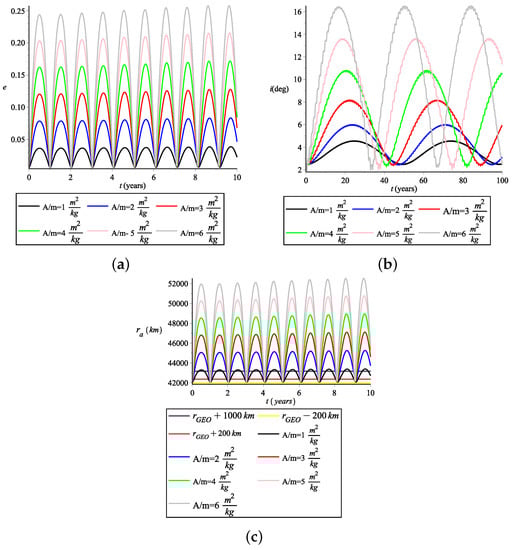
Figure 3.
Case 2. Payload object: TITAN 3C TRANSTAGE DEB-1968-081H. Initial conditions: km, , , , . Disturbing potential: . Period of integration: (a) 10 years; (b) 100 years; (c) 10 years.
Figure 3b shows the variation in the inclination for six values of . As in Case 1, there are large variations in this orbital element. Figure 3c shows that the debris takes a certain amount of time (around half the year) to reach a height largerenough to enter the defined region of the graveyard orbit, here defined as 1000 km above the GEO region. This time can be smaller for other values of (), as shown in Figure 4b. The map in Figure 4a shows the amplitude of the eccentricity when varying the angles g and h. The reddest region is the one with the largest variation in eccentricity, but the debris already enters the graveyard orbit for smaller eccentricity values, as we can see in Figure 4a,b. Finally, analyzing the two cases, we can verify the possibility of removing space debris from the GEO region to a graveyard orbit using a small solar sail, unlike the case analyzed in [27], in which the authors conducted a study to remove debris from the GEO region by pushing the object towards Earth to be incinerated in the Earth’s atmosphere. Since a large solar sail is needed to carry out the removal, then it is more complicated, in terms of technical feasibility, to use the solar sail to clean the space environment. In any case, the authors show that it is also possible to use the solar sail to reenter the GEO debris, but it will be necessary to consider an extremely large solar sail such that the SRP can increase the eccentricity so that the debris approaches the reentry zone. In the case of debris removal to the graveyard orbit, a value of = 1 m/kg is required, which is technically feasible with the existing technology. In [39], the sizes and shapes of the solar sails are discussed according to the available technology.
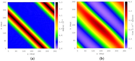
Figure 4.
Case 2. Payload object: TITAN 3C TRANSTAGE DEB-1968-081H. Initial conditions: km, , . Parameters: and steps of , and steps of . Disturbing potential: . . Time of integration: 5 years, m/kg. (a) Color bar is given by ; (b) Color bar is the time () to obtain the eccentricity in (a).
Case 3: Now, we present the results for the case where the space debris will be directed to the reentry region, that is, close to Earth’s atmosphere, to be incinerated. Since the “stuffin.space” site does not provide the data for the perigee argument g and the longitude of the ascending node h of the debris, we show diagrams of g versus h for a range of variation from to 360 (see figure legends) to see if these orbital elements can contribute to an increase in the eccentricity. Figure 5a,b show, through dynamical maps, the amplitude of the eccentricity represented in the vertical color bar. Reference [27] shows the values of the solar sail’s relation such that the debris approaches the Earth’s atmosphere, increasing its eccentricity due to the SRP acting on the sail. Thus, we choose the parameter based on this work, namely, m/kg.
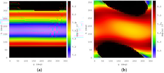
Figure 5.
Case 3. Payload object: EXPRESS 2A. Initial conditions: km, . Parameters: and steps of , and steps of . Disturbing potential: . Time of integration: 5 years, , m/kg. . (a) Real eccentricity ; (b) Fictitious eccentricity .
Figure 5a shows that an object that presents a quasi-zero eccentricity (0.002) is strongly disturbed when taking into account a solar sail coupled to the object. Note that the amplitude of the eccentricity grows considerably until the object reenters the Earth’s atmosphere, and this goal is achieved in the red regions. However, we observe that, for certain initial values of the longitude of the ascending node, and by means of the variations of the argument of perigee from zero to 360 degrees, we obtain constant ranges. However, we notice that, when we change the eccentricity of the object to 0.05, Figure 5b shows that these bands are destroyed and more complex regions appear in the dynamics. This means that, for objects in circular or near-circular orbits, the effects of the disturbing forces are even more accentuated. These results present a significant importance for the case of debris in the GEO region, as many of these bodies have almost zero eccentricities. Another point observed is that the presence of perturbations destroys completely the symmetry of the orbits. It is worth mentioning that in the most realistic case, where the Earth’s atmosphere is present, when the object is excited, especially by the SRP, the eccentricity is strongly disturbed, so the SRP lowers the perigee of the debris orbit and consequently, with the friction of atmospheric drag, the debris does not return to the same apogee. In this way, it reduces the altitude of the orbit until the debris is incinerated.
The characteristic of the orbital evolution of the debris is similar to the one appearing in Figure 5b. From these figures, it is possible to identify the values in which the orbit of the debris is more unstable. Namely, it means that, by directing the debris to values of the argument of perigee and longitude of the ascending node chosen from the maps, we can contribute to a decrease in the time of the orbital decay of the debris. Thus, we can save on reentry time and sail cost by choosing more appropriately the mass and area of the solar sail. These aspects contribute to the sustainability of space exploration, as they provide possibilities for removing space debris while using a clean and abundant propulsion mechanism that uses the energy of the Sun.
Now, considering Figure 6a, we show the simulation data taking into account the TITAN 3C TRANSTAGE DEB 969-013D debris. Note that, for different values of (), we have different eccentricity amplitudes. In two specific regions (dark color), the debris obtains the required eccentricity value to reach the reentry region (see the eccentricity values on the scale of colors). The blue region shows the values of () that keep the orbit relatively high in eccentricity, but do not allow the debris to reach the reentry region. Figure 6a shows the conditions of that the debris must be directed to contribute to the amplification of the eccentricity and thus reenter the Earth’s atmosphere when atmospheric drag is taken into account in the dynamics. Figure 6b shows the variation in the same angles shown in Figure 6a, but now the color scale shows the time when the debris reaches the reentry region. Figure 6b shows the time when the space debris reaches the reentry zone (radius of Earth + 120 km) for the values of (), which are the reddest regions in Figure 6a. Note that only a few values of () contribute to amplifying the eccentricity, so that the debris can be directed to the reentry zone with a value of m/kg. As shown in the figure, for some values of () the debris reenters very quickly, a little over a year, while in a small band (in yellow) it takes a little more than three years for that. This analysis is very important to identify possible regions of instability where the eccentricity of the debris can grow very quickly, causing the debris to reach the reentry region at the perigee of its orbit. Depending on the value of (), the reentry time changes, as shown in the color scale of Figure 6b. In this case, the value of the ratio = 25 m/kg, which in terms of technical feasibility is not possible due to the size required for the sail. The ESA, NASA, and other space agencies are working to produce very large solar sails. Performing a more refined search, we can obtain suitable regions for the values of () in which a lower ratio can be found and that can amplify the eccentricity variations. For this, a larger number of simulations must be performed. In any case, this value will be considered high in the case of debris in GEO orbit, which, to be pushed into the region of the Earth’s atmosphere, needs a large solar sail.
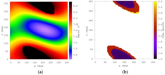
Figure 6.
Payload object: TITAN 3C TRANSTAGE. Initial conditions: km, , . Parameters: and steps of , and steps of . Disturbing potential: . . Time of integration: 5 years, m/kg. (a) Color bar is given by ; (b) Color bar is the time to obtain the eccentricity in (a).
It is worth noting that the ESA (https://www.esa.int/Enabling_Support/Space_Engineering_Technology/Shaping_the_Future/Sail_solutions_for_space_junk, accessed on 7 September 2022) is building a prototype solar sail with an area of 25 m, which would be suitable for a spacecraft weighing around 700 kg. Moreover, according to the ESA, the sail can be increased or reduced to meet the requirements, but it will always be very light and economical compared to the fuel required for a controlled de-orbit maneuver. Although at the end of the mission, or after a failure, the spacecraft may be tipping over, various aerothermodynamic calculations have shown that it is safe to deploy the sail and that the satellite will slowly self-stabilize without the need for an expensive guidance, navigation, and added control system. Another advantage is that the entire subsystem, especially the spark plug membrane, burns out very easily on reentry into the atmosphere, which is important for not falling to Earth. NASA (https://science.nasa.gov/technology/technology-highlights/solar-sail-propulsion-enabling-new-destinations-for-science-missions, accessed on 7 September 2022) is developing the 1653 m Solar Cruiser solar sail system for in-flight demonstration in 2025. NASA (https://www.nasa.gov/directorates/spacetech/small_spacecraft/ACS3, accessed on 7 September 2022) has developed a technology that can be used in future missions for solar sails up to 500 square meters, approximately the size of a basketball court. According to NASA, the technology now under development will allow solar sails of up to 2000 m.
Additionally, in order to analyze the eccentricity behavior (see Figure 7) considering the information provided by the ESA and NASA, we used the values of 25 m, 1653 m, and 2000 m for a mass of 700 kg. Note that these area-to-mass relationships are small, as shown in the legend of Figure 7. Considering this type of sail, it is possible to redirect the satellite (debris) to a graveyard orbit, as we can observe in Figure 1 and Figure 2. However, in the case of sending the debris to a region where the atmospheric drag plays a significant role, these area-to-mass values do not contribute to achieving this objective. As we can see in Figure 6, the eccentricity is more affected by the SRP for a high area-to-mass value, and thus, the solar sail contributes to lowering the perigee of the orbit while the atmospheric drag contributes to the non-return of the debris to the same position. Finally, a detail worth mentioning is that by decreasing the value of the mass it is possible to obtain a larger value of area-to-mass, enabling then the reentry of the satellite (debris).
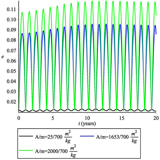
Figure 7.
Initial conditions: km, , , , . Disturbing potential: . Time of integration: 20 years, m/kg, m/kg, m/kg.
4. Conclusions
Given that, currently, the amount of space debris in Earth’s orbit already presents a very alarming number, which may make space exploration infeasible in the near future, in this study we show an option for the mitigation of space debris using a solar sail coupled to the satellite (debris) in GEO. We consider the main disturbing forces to analyze the dynamics of a solar sail coupled to the satellite, so that these perturbations, in particular the SRP, contribute to the removal of these objects from the Earth’s orbit. We show colour maps that can be useful in choosing the orbital parameters where the debris should be directed to help increase the eccentricity growth and bring the debris closer to Earth’s atmosphere to be incinerated or send the debris into a graveyard orbit. These mitigation parameters are the argument of the perigee (g), the longitude of the ascending node (h), and the area-to-mass ratio. We present results showing that it is possible to use a small solar sail ( m/kg) to direct the debris into a graveyard orbit. In this way, with an adequate choice of a pair (), we can reduce the debris reentry time, choose the appropriate value of the area-to-mass parameter, or send it into a graveyard orbit. Choosing the appropriate value of the area-to-mass parameter will reduce the costs of the solar sail. With this, we intend to contribute to the mitigation of the risks caused by space debris in a sustainable way through a clean propulsive mechanism that uses a source of energy that is also clean and abundant, namely the energy of the Sun.
Author Contributions
Conceptualization, J.P.S.C.; Methodology, J.P.S.C. and J.C.d.S.; Software, J.P.S.C., J.C.d.S., J.S.L. and L.F.B.; Validation, J.S.L. and L.F.B.; Formal analysis, J.P.S.C., J.C.d.S. and A.F.B.A.P.; Investigation, J.P.S.C. and J.C.d.S.; Writing – original draft, J.P.S.C. and J.C.d.S.; Writing—review & editing, J.C.d.S., J.P.S.C. and A.F.B.A.P.; Visualization, J.C.d.S.; Project administration, J.P.S.C.; Funding acquisition, A.F.B.A.P. All authors have read and agreed to the published version of the manuscript.
Funding
JCS thanks financial support from ITA/CAPES through a CAPES-PRINT Young Talent fellowship (Contract No 88887.583120/2020-00) and acknowledges the support of ISAS/JAXA and financial support from the Japan Society for the Promotion of Science (JSPS) through a Postdoctoral Fellowship. JSL thanks UFRB for a PIBIC fellowship. LFB and AFBAP thank the financial support from Brazil’s National Council for the Improvement of Higher Education (CAPES)—Finance Code 001. The authors wish to express their appreciation for the support provided by grant No 309089/2021-2 from the National Council for Scientific and Technological Development (CNPq), grant No. 2016/24561-0 from the São Paulo Research Foundation (FAPESP). This publication has been supported by the RUDN University Scientific Projects Grant System, project No. 202235-2-000.
Data Availability Statement
The data used in this work are avaiable to the public using the references and links provided in the manuscript.
Conflicts of Interest
The authors declare no conflict of interest.
References
- IADC (Inter-Agency Space Debris Coordination Committee). Space Debris Mitigation Guideline; IADC: Houston, TX, USA, 2007. [Google Scholar]
- Klinkrad, H. Space Debris. Models and Risk Analysis; Springer: Berlin/Heidelberg, Germany, 2006. [Google Scholar]
- ESA. ESA’s Annual Space Environment Report; ESA: Darmstadt, Germany, 2018; Issue 2; pp. 1–70. [Google Scholar]
- Formiga, J.K.S.; Santos, D.P.S.; Fiore, F.A.; Vilhena de Moraes, R.; Prado, A.F.B.A. Study of collision probability considering a non-uniform cloud of space debris. Comput. Appl. Math. 2020, 39, 21. [Google Scholar] [CrossRef]
- Kessler, D.; Cour-Palai, B.G. Collision Frequency of Artificial Satellites: The Creation of a Debris Belt. J. Geophys. Res. 1978, 83, 2637–2646. [Google Scholar] [CrossRef]
- Perek, L. Outer Space Activities versus Outer Space. J. Space Law 1979, 7, 115–119. [Google Scholar]
- Portree, V.V.S.; Loftus, J.P. Orbital Debris: A Chronology. In NASA STI/Recon Technical Report N; NASA: Washington, DC, USA, 1999. [Google Scholar]
- Kessler, D.J. Collisional Cascading: The Limits of Population Growth in Low Earth Orbit. Adv. Space Res. 1991, 11, 63–66. [Google Scholar] [CrossRef]
- Alessi, E.A.; Schettino, G.; Rossi, A.; Valsecchi, G.B. Solar radiation pressure resonances in low earth orbits. Mon. Not. R. Astron. Soc. 2018, 473, 2407–2414. [Google Scholar] [CrossRef]
- Casanova, D.; Petit, A.; Lemaître, A. Long-term evolution of space debris under the J2 effect, the solar radiation pressure and the solar and lunar perturbations. Celest. Mech. Dyn. Astron. 2015, 123, 223–238. [Google Scholar] [CrossRef]
- Gkolias, I.; Colombo, C. Towards a sustainable exploitation of the geosynchronous orbital region. Celest. Mech. Dyn. Astron. 2019, 131, 19. [Google Scholar] [CrossRef]
- Skoulidou, D.K.; Rosengren, A.J.; Tsiganis, K.; Voyatzis, G. Medium Earth Orbit dynamical survey and its use in passive debris removal. Adv. Space Res. 2019, 63, 3646–3674. [Google Scholar] [CrossRef]
- ESA. ESA’s Annual Space Environment Report; ESA: Darmstadt, Germany, 2022; Issue 6; pp. 1–120. [Google Scholar]
- NASA. History of On-Orbit Satellite Fragmentations. InOrbital Debris Program Office, 13th ed.; NASA: Washington, DC, USA, 2004. [Google Scholar]
- McInnes, C.R. Solar Sailing: Technology, Dynamics and Mission Applications; Springer-Praxis Series in Space Science and Technology; Springer: Berlin/Heidelberg, Germany, 1999. [Google Scholar]
- Herbeck, L.; Sickinger, C.; Eiden, M.; Leipold, M. Solar Sail Hardware Developments. In Proceedings of the European Conference on Spacecraft Structures, Materials and Mechanical Testing, Toulouse, France, 15–17 December 2002. [Google Scholar]
- Vilhena de Moraes, R. Combined solar radiation pressure and drag effects on the orbits of artificial satellites. Celest. Mech. 1981, 25, 281–292. [Google Scholar] [CrossRef]
- Brouwer, D.; Clemence, G.M. Methods of celestial Mechanics; Academic Press: New York, NY, USA, 1961; p. 595. [Google Scholar]
- Hori, G.I. A new approach to the solution of the main problem of the lunar theory. Astr. J. 1963, 68, 125–146. [Google Scholar] [CrossRef]
- Prado, A.F.B.A. Third-body perturbation in orbits around natural satellites. J. Guid. Control. Dyn. 2003, 26, 33–40. [Google Scholar] [CrossRef]
- Domingos, R.C.; Vilhena de Moraes, R.; Prado, A.F.B.A. Third-body perturbation in the case of elliptic orbits for the disturbing body. Math. Probl. Eng. 2008, 2008, 763654. [Google Scholar] [CrossRef]
- Cardoso dos Santos, J.; Carvalho, J.P.S.; Prado, A.F.B.A.; Vilhena de Moraes, R. Lifetime maps for orbits around Callisto using a double-averaged model. Astrophys. Space Sci. 2017, 367, 227. [Google Scholar] [CrossRef]
- Cinelli, M.; Ortore, E.; Christian Circi, C. Long Lifetime Orbits for the Observation of Europa. J. Guid. Control. Dyn. 2018, 42, 123–135. [Google Scholar] [CrossRef]
- Baresi, N.; Dell’Elce, L.; Cardoso dos Santos, J.; Kawakatsu, Y. Orbit Maintenance of Quasi-satellite Trajectories via Mean Relative Orbit Elements. In Proceedings of the International Astronautical Congress, Jerusalem, Israel, 12–16 October 2018. [Google Scholar]
- Baresi, N.; Dell’Elce, L.; Cardoso dos Santos, J.; Kawakatsu, Y. Long-term evolution of mid-altitude quasi-satellite orbits. Nonlinear Dyn. 2020, 99, 2743–2763. [Google Scholar] [CrossRef]
- Tresaco, E.; Elipe, A.; Carvalho, J.P.S. Frozen orbits for a solar sail around Mercury. J. Guid. Control. Dyn. 2016, 39, 1659–1666. [Google Scholar] [CrossRef]
- Carvalho, J.P.S.; Vilhena de Moraes, R.; Prado, A.F.B.A. Analysis of the orbital evolution of space debris using a solar sail and natural forces. Adv. Space Res. 2022, 70, 125–143. [Google Scholar] [CrossRef]
- Krivov, A.V.; Sokolov, L.L.; Dikarev, V.V. Dynamics of Mars-orbiting dust: Effects of light pressure and planetary oblateness. Celest. Mech. Dyn. Astron. 1995, 63, 313–339. [Google Scholar] [CrossRef]
- Celestino, C.C.; Winter, O.C.; Prado, A.F.B.A. Debris perturbed by radiation pressure: Relative velocities across circular orbits. Adv. Space Res. 2004, 34, 1177–1180. [Google Scholar] [CrossRef]
- Colombo, C.; Lücking, C.; McInnes, C.R. Orbital dynamics of high area-to-mass ratio spacecraft with J2 and solar radiation pressure for novel earth observation and communication services. Acta Astronaut. 2012, 81, 137–150. [Google Scholar] [CrossRef]
- Rosengren, A.J.; Scheeres, D.J. Long-term dynamics of high area-to-mass ratio objects in high-Earth orbit. Adv. Space Res. 2013, 52, 1545–1560. [Google Scholar] [CrossRef]
- Hubaux, C.; Lemaître, A. The impact of Earth‘s shadow on the long-term evolution of space debris. Celest. Mech. Dyn. Astron. 2013, 116, 79–95. [Google Scholar] [CrossRef]
- Tseng, T.-P. A Hybrid ECOM Model for Solar Radiation Pressure Effect on GPS Reference Orbit Derived by Orbit Fitting Technique. Remote Sens. 2021, 13, 4681. [Google Scholar] [CrossRef]
- Tang, L.; Wang, J.; Zhu, H.; Ge, M.; Xu, A.; Schuh, H. A Comparative Study on the Solar Radiation Pressure Modeling in GPS Precise Orbit Determination. Remote Sens. 2021, 13, 3388. [Google Scholar] [CrossRef]
- Xia, F.; Ye, S.; Chen, D.; Tang, L.; Wang, C.; Ge, M.; Neitzel, F. Advancing the Solar Radiation Pressure Model for BeiDou-3 IGSO Satellites. Remote Sens. 2022, 14, 1460. [Google Scholar] [CrossRef]
- Celletti, A.; Vartolomei, T. Old perturbative methods for a new problem in Celestial Mechanics: The space debris dynamics. Boll. Unione. Mat. Ital. 2023, in press. [Google Scholar] [CrossRef]
- Carvalho, J.P.S.; Yokoyama, T.; Mourão, D. Single-averaged model for analysis of frozen orbits around planets and moons. Celest. Mech. Dyn. Astron. 2022, 134, 35. [Google Scholar] [CrossRef]
- Carvalho, J.P.S.; Cardoso dos Santos, J.; Prado, A.F.B.A.; Vilhena de Moraes, R. Some characteristics of orbits for a spacecraft around Mercury. Comput. Appl. Math. 2018, 37, 267–281. [Google Scholar] [CrossRef]
- Miguel, N.; Colombo, C. Deorbiting spacecraft with passively stabilised attitude using a simplified quasi-rhombic-pyramid sail. Adv. Space Res. 2021, 67, 2561–2576. [Google Scholar] [CrossRef]


Disclaimer/Publisher’s Note: The statements, opinions and data contained in all publications are solely those of the individual author(s) and contributor(s) and not of MDPI and/or the editor(s). MDPI and/or the editor(s) disclaim responsibility for any injury to people or property resulting from any ideas, methods, instructions or products referred to in the content. |
© 2023 by the authors. Licensee MDPI, Basel, Switzerland. This article is an open access article distributed under the terms and conditions of the Creative Commons Attribution (CC BY) license (https://creativecommons.org/licenses/by/4.0/).