Abstract
In this paper, a three-dimensional subspace method is proposed, in which the search direction is generated by minimizing the approximation model of the objective function in a three-dimensional subspace. The approximation model of the objective function is not unique, and alternatives can be chosen between a symmetric quadratic model and a conic model by specific criteria. Moreover, the idea of a WLY conjugate gradient method is applied to characterize the change of gradient direction between adjacent iteration points. The strategy of initial stepsize and nonmonotone line search are adopted, and the global convergence of the presented algorithm is established under mild assumptions. In numerical experiments, we use a collection of 80 unconstrained optimization test problems to show the competitive performance of the presented method.
1. Introduction
Considering the following unconstrained optimization problem:
with an initial point , the following iterative formula is often used to solve (1):
where is the kth iteration point, is the stepsize determined by a line search procedure, and is the search direction obtained by special ways.
The search direction of the conjugate gradient (CG) methods is obtained by
where , and is a scalar called the conjugate gradient parameter. Corresponding to different choices for the parameter , various nonlinear conjugate gradient methods have been proposed. Some classical CG methods include HS method (Hestenes and Stiefel [1]), FR method (Fletcher and Reeves [2]), PRP method (Polak et al. [3]), CD method (Fletcher [4]), LS method (Liu and Storey [5]) and DY method (Dai and Yuan [6]).
Among these mentioned CG methods, the PRP, HS and LS methods share the common numerator , where . When the step is small, the factor tends to zero, so becomes small and the next search direction is essentially the steepest descent direction which can avoid jamming. Hence, these methods have better numerical performance than those lacking in . However, the PRP, HS and LS methods possess weak convergence properties. Based on the PRP method, Wei et al. [7] proposed a new formula
where and denotes the Euclidean norm. When step is small, also tends to zero so that the WYL method can also avoid jamming. Moreover, can avoid the drawback: if the gradients of and are significantly different, the structure of makes the smaller one between and nearly insignificant so that the method cannot make full use of the information. Furthermore, the WYL method not only has nice numerical performance but also has global convergence properties. More applications and properties of can be found in [7,8,9,10,11,12,13].
The procedure for determining the stepsize used in (2) is usually called line search, which can be classified into an exact one and an inexact one. One of the most used inexact line search is the so-called standard Wolfe line search [14]:
where . Obviously, it is a monotone procedure that seeks a suitable , making the function value decrease to some extent. Zhang and Hager [15] proposed a nonmonotone version (ZH line search) that modifies condition (4) to
where , , and are updated by
where and . The choice of controls the degree of nonmonotonicity. Such a line search can not only overcome some drawbacks in the monotone line search, but is particularly efficient for unconstrained problems in numerical experiments [15]. In addition to ZH line search, there are many other efficient nonmonotone line search procedures, which can be found in [16,17,18,19,20,21,22,23,24,25].
The subspace technique is one of the effective means for solving large-scale optimization problems, which is receivinging more and more attention. Yuan reviewed various subspace techniques that have been used in constructing numerical methods for solving nonlinear optimization problems in [26,27]. There are many optimization methods adopting the subspace technique, such as the limited-memory quasi-Newton method [28], the subspace trust region methods [29,30], the subspace SQP method [31], and more research can be found in [32,33,34,35,36,37,38]. Moreover, the combination between subspace technique and conjugate gradient method has been extensively studied. In the earliest research (see [39]), Yuan and Stoer computed the search direction by minimizing the approximation quadratic model in the two dimensional subspace spanned by and , namely where , and proposed the subspace minimization conjugate gradient method (SMCG), in which is formed by
where t and are undetermined parameters. Based on the above idea, Andrei [40] extended the subspace to and exploited the acceleration scheme, finally presenting a three-term conjugate gradient method (TTS), in which
and , are also scalar parameters. Inspired by Andrei, Yang et al. [41] changed the subspace into , and put forward the subspace three-term conjugate gradient method (STT). For the same subspace, Li et al. [42] added more parameters to the computation of search direction so that
and adopted the strategy of nonmonotone line search, eventually proposing the subspace minimization conjugate gradient method with nonmonotone line search (SMCG_NLS). Huo et al. [13] combined the idea of the WYL method with subspace method, then constructed the subspace , in which
and finally proposed a new three-dimensional subspace conjugate gradient method (TSCG).
On the other hand, Dai and Kou [43] also focused on the analysis of Yuan and Stoer, but they paid more attention to the estimate of the parameter during the calculation of . They combined the Barzilai–Borwein [44] idea and provided some efficient Barzilai–Borwein conjugate gradient methods (BBCG). It is remarkable that the idea of BBCG to estimate is employed in this paper.
It is noteworthy that all of the above mentioned subspace minimization conjugate gradient methods obtain the search direction by minimizing the approximate quadratic model of objective function in the presented subspace. However, Sun and Yuan [45,46] have pointed out that, when the current iterative point is not close to the minimizer, the quadratic model may lead to a poor prediction of the minimizer if the objective function possesses strong non-quadratic behavior. Furthermore, a quadratic model does not take into account more information instead of the gradient value in the current iteration, which means that it does not have enough degrees freedom for incorporating all of the information in the iterative procedure.
Thus, the research for approximate nonquadratic model is of the essence. Up to now, many nonquadratic models have been applied to optimization problems, such as conic model, tensor model and regularization model. The conic model can incorporate more function information than the quadratic model, and its application in unconstrained optimization was first studied by Davidon [47]. A typical conic model for unconstrained optimization is
which is an approximation to , and is a symmetric positive definite matrix approximating to the Hessian of at which satisfies the secant equation . The vector is normally called the horizontal vector satisfying . Such a conic model has been investigated by many scholars. Sorensen [48] discussed a class of conic methods called “optimization by collinear scaling” for unconstrained optimization and shown that a particular member of this algorithm class has a Q-superlinear convergence. Ariyawansa [49] modified the procedure of Sorensen [48] and established the duality between the collinear scaling DFP and BFGS methods. Sheng [50] further discussed the interpolation properties of conic model method. Di and Sun [51] proposed a trust region method for conic models to solve unconstrained optimization problems. The trust region methods based on conic model have brought about a great number of research.
Li et al. [52] paid attention to the combination of subspace method and conic model. They considered the following conic approximation model:
where
In the two-dimensional subspace , they minimized the above conic model to compute the search direction, and finally developed a subspace minimization conjugate method based on the conic model (SMCG_Conic). Sun et al. [53] extended the subspace to and presented a three-dimensional subspace minimization conjugate gradient method based on a conic model (CONIC_CG3).
The adoption of a nonquadratic model does not mean abandoning the quadratic model; here we refer to the analysis of Yuan [54], in which a quantity is defined by
which shows the extent of how the objective function is close to a quadratic on the line segment between and . Dai et al. [55] indicate that if the following condition
holds, where are two small constants, then they think that is very close to a quadratic on the line segment between and . If the condition (10) is satisfied, then the choice of the quadratic approximation model is preferable; otherwise, the conic model is more suitable. The utilization of such a quantity can be found in [56,57].
Since the combination of subspace technique and conic model has been investigated, we come up with the idea of whether we can make further studies. SMCG_Conic and CONIC_CG3 are efficient methods that possess good theoretical and numerical results, but they only considered the two-dimensional subspace and three-dimensional subspace , respectively. Hence, we expect to extend the application of conic model in the subspace conjugate gradient method. In addition, the WYL method with the ingredient has good performance both in theory and numerical experiment, and the subspace method TSCG based on quadratic model and subspace also is an efficient method. In this paper, we investigates a new application of WYL method and subspace method based on the conic model by extending SMCG_Conic to subspace . Furthermore, we adopt the initial stepsize strategy and nonmonotone line search, under which we establish the sufficient descent property and global convergence property. Since our method is based on three-dimensional subspace and conic model, it has efficient performance in numerical experiment and can solve more problems than subspace method based on two-dimensional subspace and quadratic model.
This paper is organized as follows: in Section 2, the search directions on the subspace based on two different models are derived, and the criteria for how to choose the approximate model and search direction are presented. In Section 3, we obtain the stepsize by the strategies of initial stepsize and nonmonotone line search, and elaborate the generated algorithm. In Section 4, we give the proofs for some important lemmas of the search direction, then state the convergence performance of the generated algorithm under suitable assumptions. In Section 5, we compare the numerical results of our algorithm with another two methods.
2. The Search Direction
For an optimization method, the search direction attaches great importance to the iterative formula, and the computation of search direction is always the first job. Hence, the main content of this section is to construct the formula for the search direction. Since the approximation model is selected between conic model and quadratic model, the computation will be divided into two parts.
2.1. Conic Model
In this subsection, we will give the computation of the search direction in the case that conic model is used.
When (10) is violated, the conic model is more suitable to approximate the objective function, so we compute the search direction by minimizing the conic model in subspace . We consider the subproblem
where is the same as (9).
The discussion will be divided into three parts depending on the three different dimensions of the subspace .
Situation 1:
In this situation, the search direction is
To solve (13), we first figure out the zero solution of the function
and obviously is invertible, so the problem is reduced to . After calculation, we can deduce that, when is positive definite and , the solution of (13) is
By using the relationship , where
is the adjugate matrix of , and denote the cofactor of , , respectively, in which denotes the ij-th element of and
then we finally obtain the solution of (13),
where
So the solution of (11) in the three-dimensional subspace is
During evaluation, it is important to find appropriate ways to estimate and in order to avoid matrix–vector multiplication and improve efficiency. Yuan and Stoer [39] proposed two ways to calculate such quantities containing , one of which is to obtain by using the scaled memoryless BFGS formula. The approach of Dai and Kou [43] is to combine the Barzilai–Borwein [44] idea by approximating the Hessian by or , where
For , we utilize the memoryless BFGS formula to obtain so that
Then for , we combine the idea of [42,43], and estimate by
where
and . It is obvious that .
For the estimate of , we adopt the idea of Li et al. [42], because it can guarantee some good properties. Firstly, according to the analysis regarding (14), the positive definitiveness of is essential, which requires . It follows that
By setting with , and combining (15), we have
if and only if is positive, which can be guaranteed by (18). In addition, the positive definitiveness of also requires that its first and second order leading principal minors are positive, and it means
Secondly, is also a necessary condition to keep the sufficient descent property, from which follows
if , where
and
Likewise, we define the right-hand side of (22) as , i.e., .
After the above discussion, we can estimate as follows,
where ,
and is the same as that in (18). One of the purposes of K is to ensure (21).
Before computing by (12) and (16), we should verify the following conditions:
where and are positive constants. The expressions (24) and (25) are fundamental premises of the conic model (5) and relation (22), respectively. On the basis of the Barzilai–Borwein [44] idea, (26) might indicate the suitable condition numbers of the approximation Hessian matrix. Moreover, (27) is vital to guarantee the descent property of the search direction. As for (28), obviously it makes more positive definite, and is also important for establishing the sufficient descent property of the search direction.
For convenience, we call (24)–(28) the first conic model conditions. Hence, if the first conic model conditions hold, then we compute the search direction by (12) and (16).
Situation 2:
or 1.
Li et al. [52] have made a deep study of the subspace conjugate gradient method based on the conic model in this case. Here we refer to their works. When , the search direction is formed by
which is the same as (8). The solution of t and is
which is the same as (13) in [52].
In this case, conditions (24) and (26) are still essential, but before obtaining by (8) and (29), the following conditions are also necessary:
where , is a positive constant and is identical to that in (27). We call (24), (26) and (30)–(32) the second conic model conditions. If the first conic model conditions do not all hold but the second conic model conditions hold, we compute the search direction by (8) and (29).
2.2. Quadratic Model
The content of this subsection is to calculate the search direction in the case that the objective function is approximated by a quadratic model.
When the condition (10) holds, the quadratic approximation model seems to perform well in approximating the objective function, so we consider the subproblem based on the quadratic approximation model as follows:
and related work can be found in [13]. The corresponding results can be applied to this situation. We state the concrete results in the following.
When the quadratic model conditions hold,
where
When (37) does not holds but the HS conditions hold,
Otherwise,
To sum up, the generated directions possess several forms as follows:
3. The Stepsize and Algorithm
In this section, we will present the obtainment of another essential ingredient in the iterative formula of optimization method, i.e., stepsize. It requires two steps: the first is the choice of initial stepsize, and the second is the line search procedure. After these discussion, then we can propose our whole algorithm.
3.1. Strategy for the Initial Stepsize
Firstly, we show how to choose the initial stepsize.
It is generally acknowledged that the initial stepsize is of great significance for an optimization method, especially for the conjugate gradient method. For Newton and quasi-Newton methods, the choice of the initial trial stepsize may always be unit step . However, it is different for methods that do not produce well-scaled search directions, such as the steepest descent or the conjugate gradient methods. Thus, it is significant to make a reasonable initial guess of the stepsize by considering the current information about the objective function and algorithm for such methods [58,59]. Many strategies of the initial stepsize have been proposed which can be found in the achievements of Hager and Zhang [60], Nocedal and Wright [58], Dai and Kou [19], Liu and Liu [57].
In the strategy of [19], Dai and Kou presented a condition,
where are small positive constants, denotes the initial trial stepsize, and . If condition (42) holds, it implies that the points and are not far away from each other, so it is reasonable to use the minimizer of the quadratic interpolation function for , and as the new initial stepsize, where denotes the first derivative of .
In this paper, the selection of the initial stepsize has two parts, depending on whether the negative gradient direction is adopted or not, and is presented via modification of that in Liu and Liu [56].
When the search direction is negative gradient direction, according to the analysis of Liu and Liu [57], it is desirable to take the initial trial stepsize by
where and are two positive constants controlling the initial stepsize within the interval which is preferable in numerical experiments.
Andrei [61] thinks that, the more accurate the step length is, the faster convergence a conjugate gradient algorithm has. It therefore makes sense to verify if the initial trial stepsize satisfies (42) or not. If so and , , we update the initial stepsize by
where
where denotes the quadratic interpolation function for , and .
Therefore, the initial stepsize for the negative gradient direction is
When it comes to the search direction that is not negative gradient direction, the similarity of the calculation between our direction and that in quasi-Newton methods implies that the unit stepsize might be a reasonable initial trial stepsize. Again we figure out the minimizer of the quadratic interpolation function
If satisfies (42) and , we update the initial stepsize by
Therefore, the initial stepsize for the search direction except negative gradient direction is
3.2. The Nonmonotone Line Search
Secondly, we introduce the line search used in our algorithm.
For the variable in ZH line search, Zhang and Hager [15] proved that if , then the generated sequence only has the property that
Liu and Liu [57] presented a formula of ,
where and denotes the residue for k modulo n, and it resulted in a better convergence.
Referring to the above study, Li et al. [52] and Sun et al. [53] made some modifications so that the improved line search is more appropriate for their algorithms.
In order to gain the decent convergence result and performance, this paper modifies the improved ZH line search used in [53]. To be specific, we set
where
where .
3.3. Algorithm
In this subsection, we will detail our new three-dimensional subspace method based on conic model.
First, we incorporate a special restart technique proposed by Dai and Kou [19]. They defined a quantity
where and . If is close to 1, they think that the line search function is close to some quadratic function. According to their analysis, the exact approach of this quantity is that if there are continuously many iterations such that is close to 1, we restart the algorithm with the negative gradient direction. In addition, if the number of the iterations since the last restart reaches the MaxRestart threshold, we also restart out algorithm.
The details of the three-dimensional subspace conjugate gradient method based on conic model are given in the next algorithm, which is Algorithm 1.
| Algorithm 1 WYL_TSCO |
Require: initial point , initial stepsize , positive constants |
Ensure: optimal |
|
4. Properties of the Proposed Algorithm
The theoretical nature is an important criterion to determine the performance of an algorithm. In this section, we will give some properties of WYL_TSCO, including the sufficient descent property and the global convergence.
4.1. Some Lemmas
This subsection will make a deep discussion on our algorithm and prove some properties of the presented directions before establishing the global convergence. At first, we propose two assumptions as follows:
Assumption A1.
The objective function is continuously differentiable and bounded from below on .
Assumption A2.
The gradient function is Lipschitz continuous on the level set , which means that there exists a positive constant satisfying
which implies that.
With these assumptions, we can prove some properties of the new directions in the following.
Lemma 1.
For the search direction calculated by WYL_TSCO, there exists a constant such that
Proof.
We will discuss in several parts based on different situations and different approximation models.
Case I: if the negative direction is adopted, i.e., , then
Case III (conic): if is calculated by (8) and (29), Li, Liu and Liu [52] have proved that
where
and is a positive constant.
Case IV (conic): when is obtained by (12) and (16), we have
where , . Moreover, is a binary quadratic function of x and y which can be expressed as
It is easy to acquire the Hessian of
we have because is positive definite, and the determinant of
is also positive, so has a minimizer, that is
Therefore, we can derive
Because and are all positive, we just need to prove that has a lower bound. Since contains , we first prove that has an upper bound; that is the upper bound of and K.
For , we use the Cauchy inequality and can obtain
combining (17), (18) and using the Cauchy inequality again, we have
Note that , the above inequality of can be simplified to
Next, the upper bound of is acquired by the same procedure,
For , it is easy to know that
Through the above discussion, now we can give the upper bound of ,
where
Since we have found the upper bound of , then we now consider . According to (22), can be expressed as
Using the formula of and the upper bound of , we have
Note that
so the above inequality of can be simplified to
Case V (quadratic): when is generated by (8) and (41), the proof can be found in [43], in which Dai and Kou proved that
After the above discussion, we can prove that there indeed exists a constant such that
where
The proof is complete. □
Lemma 2.
Assume that f satisfies Assumption 2. If the search direction is calculated by WYL_TSCO, then there exists a constant such that
Proof.
Similar to Lemma 1, the proof is divided into several cases.
Case I: if is calculated by negative gradient, then there certainly holds
Case II: if the search direction is the HS direction, according to Assumption 2 and the condition (33), we have
Case IV (conic): if is formed by (12) and (16), we have
so in order to prove Lemma 2 in this case, we first need to obtain a lower bound of . Combining (23), (25) and (51), and the value range of , we can derive
Then using the above inequality, we can transform (56) into
Since (26) implies that , we finally obtain an upper bound of , that is
For convenience, we define
namely,
Case V (quadratic): if is formed by (8) and (41), it is similar to Lemma 4 in Li, Liu and Liu [42]. According to their proof, we can deduce
Since , we finally have
According to the above analysis, the proof of Lemma 2 is completed by setting
□
4.2. Convergence Analysis
In this subsection, we will give the global convergence of the presented algorithm for general functions.
Lemma 3.
Proof.
□
Theorem 1.
Suppose the objective function f satisfies Assumptions 1 and 2, and sequence is generated by WYL_TSCO, then we have
Proof.
With the reasonable assumptions that , , , , and according to the update formulas (7) and (48), we can acquire that
Combining (48), we can derive the general formula of ,
where denotes the floor function. Thus, it is easy to obtain an upper bound of ,
where .
Hence is monotonically decreasing. According to Lemma 1.1 in [15], we have for each , and (46) indicates that for each . Thus, with the assumption that f is bounded below, is certainly bounded from below.
Summing up the above analysis and (61), we can finally obtain that
which implies
The proof is completed. □
5. Numerical Results
In this section, the results of the numerical experiments are shown below. The unconstrained test functions were taken from [62] with the given initial points. To prove the efficiency of the proposed WYL_TSCO algorithm, we compare its numerical performance with SMCG_Conic and TSCG. The performance profile proposed by Dolan and Moré [63] is used to evaluate the performance of these methods. The dimension of the test functions is 10,000. All the programs were written in C code.
SMCG_Conic is also a subspace minimization conjugate gradient algorithm based on the conic model, and is a pioneering one that combines the subspace technique with a conic model to seek the search direction. The numerical experiments in [52] show that the performance of SMCG_Conic is very efficient. Since the biggest difference between WYL_TSCO and SMCG_Conic is the dimension of the used subspace, the comparison between WYL_TSCO and SMCG_Conic can not only reflect the high efficiency of our algorithm, but also reveal the influence on the numerical result generated by the change of dimension for the adopted subspace in the subspace minimization conjugate gradient algorithm.
As for TSCG, it is an efficient subspace minimization conjugate gradient method, and it successfully applies the idea of subspace method and WYL method which are employed in our algorithm as well. However, TSCG only uses the quadratic model to approximate the objective function. Thus, the comparison between the numerical performance of WYL_TSCO and TSCG can reveal the influence of the approximation model in the subspace method.
For the initial stepsize of the first iteration, we adopt the adaptive strategy used in [42]. The other parameters of WYL_TSCO are selected as follows.
SMCG_Conic and TSCG use the original parameters in their paper respectively. In addition to stopping when the stopping criterion holds, the algorithm also stops when the number of iterations exceeds 200,000.
For the 80 test problems from [62], WYL_TSCO successfully solves 100% of them, while TSCG and SMCG_Conic both successfully solve 76 problems. We compare the numerical results of problems that are solved successfully by all the three algorithms, the number of which are 72. The numerical results of the three algorithms are presented in the following figures.
Figure 1 depicts the performance based on the number of iterations for the three methods. It shows that the performance of WYL_TSCO is similar to that of TSCG, but is a little inferior to SMCG_Conic’s only when . However, WYL_TSCO outperforms TSCG and SMCG_Conic when .
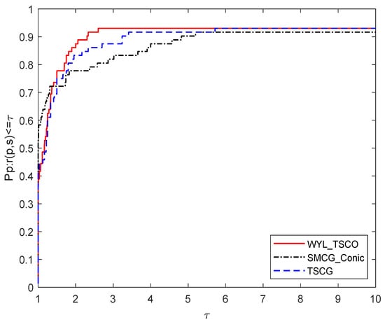
Figure 1.
Performance profile based on the number of iterations.
In Figure 2, we observe that WYL_TSCO and TSCG outperforms SMCG_Conic on the number of function evaluations, and TSCG is slightly ahead of WYL_TSCG only in the case of .
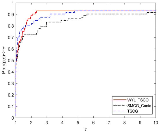
Figure 2.
Performance profile based on the number of function evaluations.
Similar to Figure 1, Figure 3 illustrates that WYL_TSCO is at a little disadvantage compared with SMCG_Conic only when , but is competitive with TSCG.
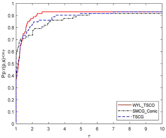
Figure 3.
Performance profile based on the number of gradient evaluations.
For the CPU time, Figure 4 shows that WYL_TSCO has an improvement on TSCG and SMCG_Conic, which shows the high efficiency of WYL_TSCO.
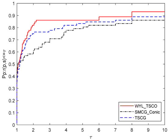
Figure 4.
Performance profile based on the CPU time.
For the 80 test problems, the numerical results show that WYL_TSCO and TSCG may perform a little worse than SMCG_Conic when is very small, but they overall have significant improvements over SMCG_Conic, and WYL_TSCO also is superior to TSCG for almost all . Moreover, WYL_TSCO can solve more problems than TSCG and SMCG_Conic, which might show the advantage of the three-dimensional subspace method and conic model. To sum up, the WYL_TSCO is an efficient algorithm for solving the unconstrained optimization problem.
6. Conclusions
Combining the idea of WYL method, this paper proposes a three-dimensional subspace method based on conic models for unconstrained optimization (WYL_TSCO). The sufficient descent property of the search direction and the global convergence of this method are obtained under some suitable assumptions. The selection of an approximation model depends on whether certain criterions are satisfied. Furthermore, the strategies of initial stepsize and nonmonotone line search are exploited which are beneficial to the convergence and efficiency. According to the numerical results and theoretical analysis, WYL_TSCO is very competitive and promising.
Author Contributions
Conceptualization, S.Y.and J.X.; methodology, G.W.; software and validation, G.W. and M.P.; visualization and formal analysis, G.W.; writing—original draft preparation, G.W.; supervision, S.Y.; funding acquisition, S.Y. and J.X. All authors have read and agreed to the published version of the manuscript.
Funding
Chinese National Natural Science Foundation no. 12262002, Natural Science Foundation of Guangxi Province (CN) no. 2020GXNSFAA159014 and 2021GXNSFAA196076, the Program for the Innovative Team of Guangxi University of Finance and Economics, and Guangxi First-class Discipline statistics Construction Project.
Institutional Review Board Statement
Not applicable.
Informed Consent Statement
Not applicable.
Data Availability Statement
Not applicable.
Conflicts of Interest
The authors declare no conflict of interest.
References
- Hestenes, M.R.; Stiefel, E.L. Methods of conjugate gradients for solving linear systems. J. Res. Natl. Bur. Stand. 1952, 49, 409–436. [Google Scholar] [CrossRef]
- Fletcher, R.; Reeves, C.M. Function minimization by conjugate gradients. Comput. J. 1964, 7, 149–154. [Google Scholar] [CrossRef]
- Polyak, B.T. The conjugate gradient method in extremal problems. Jussr Comput. Math. Math. Phys. 1969, 9, 94–112. [Google Scholar] [CrossRef]
- Fletcher, R. Volume 1 Unconstrained Optimization. In Practical Methods of Optimization; Wiley: New York, NY, USA, 1987. [Google Scholar]
- Liu, Y.L.; Storey, C.S. Efficient generalized conjugate gradient algorithms, part 1: Theory. J. Optim. Theory Appl. 1991, 69, 129–137. [Google Scholar] [CrossRef]
- Dai, Y.H.; Yuan, Y.X. A nonlinear conjugate gradient method with a strong global convergence property. Siam J. Optim. 1999, 10, 177–182. [Google Scholar] [CrossRef]
- Wei, Z.; Yao, S.; Liu, L. The convergence properties of some new conjugate gradient methods. Appl. Math. Comput. 2006, 183, 1341–1350. [Google Scholar] [CrossRef]
- Huang, H.; Wei, Z.; Yao, S. The proof of the sufficient descent condition of the Wei-Yao-Liu conjugate gradient method under the strong Wolfe-Powell line search. Appl. Math. Comput. 2007, 189, 1241–1245. [Google Scholar] [CrossRef]
- Zhang, L. An improved Wei-Yao-Liu nonlinear conjugate gradient method for optimization computation. Appl. Math. Comput. 2009, 215, 2269–2274. [Google Scholar] [CrossRef]
- Yao, S.; Qin, B. A hybrid of DL and WYL nonlinear conjugate gradient methods. Abstr. Appl. Anal. 2014, 2014, 279891. [Google Scholar] [CrossRef]
- Huang, H.; Lin, S. A modified Wei-Yao-Liu conjugate gradient method for unconstrained optimization. Appl. Math. Comput. 2014, 231, 179–186. [Google Scholar] [CrossRef]
- Hu, Y.; Wei, Z. Wei-Yao-Liu conjugate gradient projection algorithm for nonlinear monotone equations with convex constraints. Int. J. Comput. Math. 2015, 92, 2261–2272. [Google Scholar] [CrossRef]
- Huo, J.; Yang, J.; Wang, G.; Yao, S. A class of three-dimensional subspace conjugate gradient algorithms for unconstrained optimization. Symmetry 2022, 14, 80. [Google Scholar] [CrossRef]
- Wolfe, P. Convergence conditions for ascent methods. SIAM Rev. Soc. Ind. Appl. Math. 1969, 11, 226–235, Erratum in SIAM Rev. Soc. Ind. Appl. Math. 1971, 13, 185–188. [Google Scholar] [CrossRef]
- Zhang, H.; Hager, W.W. A nonmonotone line search technique and its application to unconstrained optimization. SIAM J. Optim. 2004, 14, 1043–1056. [Google Scholar] [CrossRef]
- Grippo, L.; Lampariello, F.; Lucidi, S. A nonmonotone line search technique for Newton’s method. SIAM J. Numer. Anal. 1986, 23, 707–716. [Google Scholar] [CrossRef]
- Hager, W.W.; Zhang, H. A new conjugate gradient method with guaranteed descent and an efficient line search. SIAM J. Optim. 2005, 16, 170–192. [Google Scholar] [CrossRef]
- Gu, N.Z.; Mo, J.T. Incorporating nonmonotone strategies into the trust region method for unconstrained optimization. Comput. Math. Appl. 2008, 55, 2158–2172. [Google Scholar] [CrossRef]
- Dai, Y.H.; Kou, C.X. A nonlinear conjugate gradient algorithm with an optimal property and an improved Wolfe line search. SIAM J. Optim. 2013, 23, 296–320. [Google Scholar] [CrossRef]
- Huang, S.; Wan, Z.; Chen, X. A new nonmonotone line search technique for unconstrained optimization. Numer. Algorithms 2015, 68, 671–689. [Google Scholar] [CrossRef]
- Ou, Y.; Liu, Y. A memory gradient method based on the nonmonotone technique. J. Ind. Manag. Optim. 2017, 13, 857–872. [Google Scholar] [CrossRef]
- Ahookhosh, M.; Amini, K.; Peyghami, M.R. A nonmonotone trust-region line search method for large-scale unconstrained optimization. Appl. Math. Model. 2012, 36, 478–487. [Google Scholar] [CrossRef]
- Ahookhosh, M.; Amini, K. An efficient nonmonotone trust-region method for unconstrained optimization. Numer. Algorithms 2012, 59, 523–540. [Google Scholar] [CrossRef]
- Kimiaei, M.; Rahpeymaii, F. A new nonmonotone line-search trust-region approach for nonlinear systems. TOP 2019, 27, 199–232. [Google Scholar] [CrossRef]
- Kimiaei, M. A new class of nonmonotone adaptive trust-region methods for nonlinear equations with box constraints. Calcolo 2017, 54, 769–812. [Google Scholar] [CrossRef]
- Yuan, Y.X. Subspace techniques for nonlinear optimization. In Some Topics in Industrial and Applied Mathematics; Jeltsch, R., Li, D.Q., Sloan, I.H., Eds.; Higher Education Press: Beijing, China, 2007; pp. 206–218. [Google Scholar]
- Yuan, Y.X. A review on subspace methods for nonlinear optimization. In Proceedings of the International Congress of Mathematics, Seoul, Republic of Korea, 13–21 August 2014; pp. 807–827. [Google Scholar]
- Liu, D.C.; Nocedal, J. On the limited memory BFGS method for large scale optimization. Math. Program. 1989, 45, 503–528. [Google Scholar] [CrossRef]
- Wang, Z.H.; Wen, Z.W.; Yuan, Y. A subspace trust region method for large scale unconstrained optimization. In Numerical Linear Algebra and Optimization; Yuan, Y., Ed.; Science Press: Beijing, China, 2004; pp. 265–274. [Google Scholar]
- Wang, Z.H.; Yuan, Y. A subspace implementation of quasi-Newton trust region methods for unconstrained optimization. Numer. Math. 2006, 104, 241–269. [Google Scholar] [CrossRef]
- Lee, J.H.; Jung, Y.M.; Yuan, Y.X.; Yun, S. A subspace SQP method for equality constrained optimization. Comput. Optim. Appl. 2019, 74, 177–194. [Google Scholar] [CrossRef]
- Gill, P.E.; Leonard, M.W. Reduced-hessian quasi-newton methods for unconstrained optimization. SIAM J. Optim. 2001, 12, 209–237. [Google Scholar] [CrossRef]
- Liu, X.; Wen, Z.; Zhang, Y. Limited memory block Krylov subspace optimization for computing dominant singular value decompositions. SIAM J. Sci. Comput. 2013, 35, A1641–A1668. [Google Scholar] [CrossRef]
- Yuan, Y.X. Subspace methods for large scale nonlinear equations and nonlinear least squares. Optim. Eng. 2009, 10, 207–218. [Google Scholar] [CrossRef]
- Dong, Q.; Liu, X.; Wen, Z.W.; Yuan, Y.X. A parallel line search subspace correction method for composite convex optimization. J. Oper. Res. Soc. China. 2015, 3, 163–187. [Google Scholar] [CrossRef]
- Li, Y.; Liu, H.; Wen, Z.; Yuan, Y.X. Low-rank matrix iteration using polynomial-filtered subspace extraction. SIAM J. Sci. Comput. 2020, 42, A1686–A1713. [Google Scholar] [CrossRef]
- Kimiaei, M.; Neumaier, A.; Azmi, B. LMBOPT: A limited memory method for bound-constrained optimization. Math. Prog. Comp. 2022, 14, 271–318. [Google Scholar] [CrossRef]
- Cartis, C.; Roberts, L. Scalable subspace methods for derivative-free nonlinear least-squares optimization. Math. Program. 2023, 199, 461–524. [Google Scholar] [CrossRef]
- Yuan, Y.X.; Stoer, J. A subspace study on conjugate gradient algorithms. Z. Angew. Math. Mech. 1995, 75, 69–77. [Google Scholar] [CrossRef]
- Andrei, N. An accelerated subspace minimization three-term conjugate gradient algorithm for unconstrained optimization. Numer. Algorithms 2014, 65, 859–874. [Google Scholar] [CrossRef]
- Yang, Y.; Chen, Y.; Lu, Y. A subspace conjugate gradient algorithm for large-scale unconstrained optimization. Numer. Algorithms 2017, 76, 813–828. [Google Scholar] [CrossRef]
- Li, M.; Liu, H.; Liu, Z. A new subspace minimization conjugate gradient method with nonmonotone line search for unconstrained optimization. Numer. Algorithms 2018, 79, 195–219. [Google Scholar] [CrossRef]
- Dai, Y.H.; Kou, C.X. A Barzilai-Borwein conjugate gradient method. Sci. China Math. 2016, 59, 1511–1524. [Google Scholar] [CrossRef]
- Barzilai, J.; Borwein, J.M. Two-point step size gradient methods. IMA J. Numer. Anal. 1988, 8, 141–148. [Google Scholar] [CrossRef]
- Sun, W. On nonquadratic model optimization methods. Asia. Pac. J. Oper. Res. 1996, 13, 43–63. [Google Scholar]
- Sun, W.; Yuan, Y. Optimization Theory and Methods: Nonlinear Programming; Springer: New York, NY, USA, 2006. [Google Scholar]
- Davidon, W.C. Conic Approximations and Collinear Scalings for Optimizers. SIAM J. Numer. Anal. 1980, 17, 268–281. [Google Scholar] [CrossRef]
- Sorensen, D.C. The Q-superlinear convergence of a collinear scaling algorithm for unconstrained optimization. SIAM J. Numer. Anal. 1980, 17, 84–114. [Google Scholar] [CrossRef]
- Ariyawansa, K.A. Deriving collinear scaling algorithms as extensions of quasi-Newton methods and the local convergence of DFP- and BFGS-related collinear scaling algorithms. Math. Program. 1990, 49, 23–48. [Google Scholar] [CrossRef]
- Sheng, S. Interpolation by conic model for unconstrained optimization. Computing 1995, 54, 83–98. [Google Scholar] [CrossRef]
- Di, S.; Sun, W. A trust region method for conic model to solve unconstraind optimizaions. Optim. Methods Softw. 1996, 6, 237–263. [Google Scholar] [CrossRef]
- Li, Y.; Liu, Z.; Liu, H. A subspace minimization conjugate gradient method based on conic model for unconstrained optimization. Comput. Appl. Math. 2019, 38, 16. [Google Scholar] [CrossRef]
- Sun, W.; Li, Y.; Wang, T.; Liu, H. A new subspace minimization conjugate gradient method based on conic model for large-scale unconstrained optimization. Comput. Appl. Math. 2022, 41, 178. [Google Scholar] [CrossRef]
- Yuan, Y.X. A modified BFGS algorithm for unconstrained optimization. IMA J. Numer. Anal. 1991, 11, 325–332. [Google Scholar] [CrossRef]
- Dai, Y.H.; Yuan, J.Y.; Yuan, Y.X. Modified two-point stepsize gradient methods for unconstrained optimization problems. Comput. Optim. Appl. 2002, 22, 103–109. [Google Scholar] [CrossRef]
- Liu, Z.; Liu, H. An efficient gradient method with approximate optimal stepsize for large-scale unconstrained optimization. Numer. Algorithms 2018, 78, 21–39. [Google Scholar] [CrossRef]
- Liu, H.; Liu, Z. An efficient Barzilai-Borwein conjugate gradient method for unconstrained optimization. J. Optim. Theory Appl. 2019, 180, 879–906. [Google Scholar] [CrossRef]
- Nocedal, J.; Wright, S.J. Numerical Optimization; Springer: New York, NY, USA, 2006. [Google Scholar]
- Andrei, N. Nonlinear Conjugate Gradient Methods for Unconstrained Optimization; Springer: Cham, Switzerland, 2020. [Google Scholar]
- Hager, W.W.; Zhang, H. Algorithm 851: CG_DESCENT, a conjugate gradient method with guaranteed descent. ACM Trans. Math. Softw. 2006, 32, 113–137. [Google Scholar] [CrossRef]
- Andrei, N. Open problems in nonlinear conjugate gradient algorithms for unconstrained optimization. Bull. Malays. Math. Sci. Soc. Second Ser. 2011, 34, 319–330. [Google Scholar]
- Andrei, N. An unconstrained optimization test functions collection. Adv. Model. Optim. 2008, 10, 147–161. [Google Scholar]
- Dolan, E.D.; Moré, J.J. Benchmarking optimization software with performance profiles. Math. Program. 2002, 91, 201–213. [Google Scholar] [CrossRef]


Disclaimer/Publisher’s Note: The statements, opinions and data contained in all publications are solely those of the individual author(s) and contributor(s) and not of MDPI and/or the editor(s). MDPI and/or the editor(s) disclaim responsibility for any injury to people or property resulting from any ideas, methods, instructions or products referred to in the content. |
© 2023 by the authors. Licensee MDPI, Basel, Switzerland. This article is an open access article distributed under the terms and conditions of the Creative Commons Attribution (CC BY) license (https://creativecommons.org/licenses/by/4.0/).