Scrutiny of a More Flexible Counterpart of Huang–Kotz FGM’s Distributions in the Perspective of Some Information Measures

Abstract

In this work, we reveal some distributional traits of concomitants of order statistics (COSs) arising from the extended Farlie–Gumbel–Morgenstern (FGM) bivariate distribution, which was developed and studied in recent work. The joint distribution and product moments of COSs for this family are discussed. Moreover, some useful recurrence relations between single and product moments of concomitants are obtained. In addition, the asymptotic behavior of the concomitant’s rank for order statistics (OSs) is studied. The information measures, differential entropy, Kullback–Leibler (KL) distance, Fisher information number (FIN), and cumulative past inaccuracy (CPI) are theoretically and numerically studied.

1. Introduction

A statistical model that explains the relationships between one or more random variables (RVs) and one or more other variables is any family of multivariate distributions. A family of bivariate distributions is a group of probability distributions from which one can sample a bivariate data set. The FGM family of bivariate distributions is the seminal family in this context. With this family, it is easy to comprehend how the marginals are dependent on one another, but with a correlation of ($-0.33$, 0.33). Thus, the FGM distribution can only be employed with data with a low correlation. Nevertheless, the FGM copula, a radially symmetric copula has supplanted the conventional multivariate normal models in several situations and is now widely used in many branches of study. The FGM family, for instance, was used in [1] to represent the dependence pattern in environmental and biological variables. For further details on the application of the FGM family in engineering and ecology, read Ota et al. [2]. The variants of this family were also used in [3] to simulate symmetric real-world datasets. For bivariate meta-analyses, Shih et al. [4] substituted the FGM copula and some of its symmetric and asymmetric generalizations for the bivariate normal model. The bivariate luminosity density functions in astronomy were built in [5] using the FGM copula.

Most FGM copula extensions that have been published in the literature work to boost correlation. Huang and Kotz [6] used consecutive iterations to increase the correlation between components in the traditional FGM distribution. Additionally, the first and second types of extensions given in [7] (designated by the abbreviations HK-FGM1 and HK-FGM2) offer a close correlation range. Barakat et al. [8,9] amended a new symmetric generalization of FGM copula, which was introduced in [10] (this paper was published on the line in 2020). The admissible range derived in [10] and the claim about the correlation was demonstrated to be false. The corrected admissible range of this copula was obtained in [8] and it was shown to be regarded as HK-FGM1’s counterpart in that they both have two shape parameters and offer an equal improvement over the FGM copula in terms of the positive correlation between the dependent variables. The suggested copula, as an extension of the classical FGM copula, has a simpler functional form than HK-FGM1, because to obtain it, we used an additional shape parameter as a multiplicative factor, whereas to obtain the latter, the additional shape parameter is used as an exponent. A few exceptional examples of further expansions of the FGM copula are included in the modified copula in addition to this obvious motivation.

The cumulative distribution function (CDF) and probability density function (PDF) of the new extended FGM family (denoted by HK-FGM3 or more specifically HK-FGM3$(a,b)$) are given by (cf. [8])

$$F_{X,Y}(x,y)=F_X\left(x\right)F_Y\left(y\right)\left[1+a{\overline{F}}_X\left(x\right){\overline{F}}_Y\left(y\right)(1+b{F}_X\left(x\right))(1+b{F}_Y\left(y\right))\right]$$

and

$$f_{X,Y}(x,y)=f_X\left(x\right)f_Y\left(y\right)\left\{1+a\left[C_1(x,y)+b(C_2(x,y)+C_3(x,y))+b^2{C}_4(x,y)\right]\right\},$$

(1)

where $C_1(x,y)=(1-2F_X\left(x\right))(1-2F_Y\left(y\right)),$$C_2(x,y)=(1-2F_X\left(x\right))(2F_Y\left(y\right)-3F_Y^2\left(y\right)),$$C_3(x,y)=(2F_X\left(x\right)-3F_X^2\left(x\right))(1-2F_Y\left(y\right)),$$C_4(x,y)=(2F_X\left(x\right)-3F_X^2\left(x\right))(2F_Y\left(y\right)-3F_Y^2\left(y\right)),$$f_X\left(x\right)$ and $f_Y\left(y\right)$ are the PDFs of the RVs X and Y, respectively, whereas ${\overline{F}}_X$ and ${\overline{F}}_Y$ are the survival functions (SFs). When the two marginals $F_X\left(x\right)$ and $F_Y\left(y\right)$ are continuous, Barakat et al. [8] showed that the natural parameter space Ω (the admissible set of the parameters a and b that makes $F_{X,Y}(x,y)$ is a bonafide CDF) is convex, and the set $\Omega$ is given by $\Omega ={\Omega }^{+}\cup {\Omega }^{-},$ where

$$\begin{array}{ccc}\hfill {\Omega }^{+}& =& \left\{(a,b):0\le b\le 1,-\frac{1}{{(1+b)}^2}\le a\le \frac{1}{(1+b)};\mathrm{or}b>1,-\frac{1}{{(1+b)}^2}\le a\le \frac{1}{{(1+b)}^2}\right\},\hfill \\ \hfill {\Omega }^{-}& =& \left\{(a,b):-2\le b\le 0,-1\le a\le 0;\mathrm{or}b<-2,-\frac{1}{{(1+b)}^2}\le a\le \frac{1}{{(1+b)}^2}\right\}.\hfill \end{array}$$

The generalized exponential (GE) distribution $F_X\left(x\right)={(1-e^{-\theta x})}^{\alpha },x;\alpha ,\theta >0,$ denoted by $GE(\theta ,\alpha ),$ that dates to Gupta and Kundu [11], is the one we usually use throughout this study when we have to interact with specific marginals. The exponential distribution is $GE(\theta ,1).$ Additionally, the shape and scale parameters are $\alpha$ and $\theta$, respectively. The GE is a unimodal density function, and for fixed scale parameters, as the shape parameter increases, it becomes more and more symmetric. In reliability theory, the Weibull distribution represents a series system, whereas the GE distribution describes a parallel system. In other words, if a parallel system has n components and all of their lifetimes are i.i.d. RVs that follow GE, then the system’s lifetime distribution is also GE. According to Gupta and Kundu [11], the ℓth moment of $GE(\theta ,\alpha )$ is given by

$$\begin{array}{c}\hfill {\mu }_X^{\left(𝓁\right)}=\frac{\alpha 𝓁!}{{\theta }^{𝓁}}{\displaystyle \sum _{i=0}^{\kappa (\alpha -1)}}\frac{{(-1)}^i}{{(i+1)}^{𝓁+1}}\left(\genfrac{}{}{0pt}{}{\alpha -1}{i}\right),\end{array}$$

where $\kappa \left(x\right)=\infty ,$ if x is non-integer and $\kappa \left(x\right)=x,$ if x is integer. Moreover, the mean, variance, and moment-generating function (MGF) of $GE(\theta ,\alpha )$ are given by

$$\begin{array}{c}\hfill {\mu }_X=\mathrm{E}\left(X\right)=\frac{B\left(\alpha \right)}{\theta },\mathrm{Var}\left(X\right)={\sigma }_X^2=\frac{C\left(\alpha \right)}{{\theta }^2},\mathrm{and}{M}_X\left(t\right)=\alpha \beta (\alpha ,1-\frac{t}{\theta }),\mathrm{respectively},\end{array}$$

where $B\left(\alpha \right)=\Psi (\alpha +1)-\Psi \left(1\right)$ (which is the Euler’s harmonic number), $C\left(\alpha \right)={\Psi }^{\prime }\left(1\right)-{\Psi }^{\prime }(\alpha +1),$ $\beta (a,b)=\frac{\Gamma \left(a\right)\Gamma \left(b\right)}{\Gamma (a+b)},$ and $\Psi (.)$ is the digamma function, whereas ${\Psi }^{\prime }(.)$ is its derivation (the trigamma function).

COS can emerge in sundry applications. A linked trait Y that is difficult to measure or can only be detected later may be of importance when items or persons are selected based on their X characteristic. See David and Nagaraja [12] for a thorough examination of the various applications for the COSs. Currently, a number of recent investigations, including [13], can be found in the literature for the COSs based on various generalizations of the FGM family. Suppose $(X_i,Y_i),$ $i=1,2,...,n,$ is a random sample from a bivariate CDF $F_{X,Y}(x,y).$ If we order the sample by the X-variate, and obtain the OSs, $X_{1:n}\le X_{1:n}\le ....\le X_{n:n}$, for the X sample, then the Y-variate associated with the rth OS $X_{r:n}$ is called the concomitant of the rth OS, and is denoted by $Y_{[r:n]}.$ Since the conditional PDF of $Y_{[r:n]}$ given $X_{r:n}=x$ is $f_{Y_{[r:n]}|X_{r:n}}\left(y\right|x)=f_{Y|X}\left(y\right|x),$ the PDF of $Y_{[r:n]}$ is given by

$$g_{[r:n]}\left(y\right)={\int }_{-\infty }^{\infty }{f}_{Y\mid X}(y\mid x)f_{X_{r:n}}\left(x\right)dx,$$

(2)

where $f_{X_{r:n}}\left(x\right)$ is the PDF of the rth OS $X_{r:n}$ (cf. [14]). Moreover, the joint PDF (JPDF) of the concomitants $Y_{[r:n]}$ and $Y_{[s:n]}$ of the rth and sth OSs $X_{r:n}$ and $X_{s:n},1\le r<s\le n,$ is given by

$$g_{[r,s:n]}(y_1,y_2)={\int }_{-\infty }^{\infty }{\int }_{-\infty }^{x_2}{f}_{Y|X}\left(y_1\right|x_1)f_{Y|X}\left(y_2\right|x_2)f_{r,s:n}(x_1,x_2)d{x}_{1}d{x}_2,$$

(3)

where $f_{r,s:n}(x_1,x_2)$ is the JPDF of $X_{r:n}$ and $X_{s:n}$ (cf. [13]).

In this study, we take into account four different types of information measures: differential entropy, KL distance, FIN, and CPI. Here is a quick explanation of these information measures.

The Shannon entropy is a gauge that was introduced and developed in [15] to assess the average reduction in uncertainty or variability brought on by a discrete RV. This measurement is a continuous, non-negative additive for independent occurrences, and grows as the number of possibilities with non-zero probabilities grows. It is also maximal for uniform distributions. Certain symmetry features can be found in the Shannon entropy. For instance, if the results are rearranged, the Shannon entropy remains unaffected. The symmetry and asymmetry concepts in physics are highly pertinent to this measure. Entropy is typically thought of as the quantitative measure of disorder from a physics perspective. To link “ordering” with the symmetrization of a physical system, or, in other words, the introduction of the elements of symmetry into an initially disordered physical system, is to identify the disorder as the absence of symmetry (cf. [16]). Symmetry is highly valued in contemporary science, and any differentiable symmetry of a physical system’s action is accompanied by a conservation law. One way to think about entropy reduction is through symmetry (cf. [17]). The differential entropy, often known as the corresponding measure for a continuous RV X with a PDF $f_X\left(x\right),$ and CDF $F_X\left(x\right),$ is defined by (cf. [18])

$$H\left(X\right)=-\mathrm{E}(ln{f}_X\left(X\right))=-{\int }_{-\infty }^{\infty }{f}_X\left(x\right)ln{f}_X\left(x\right)dx=-{\int }_0^{1}ln{f}_X\left(F_X^{-1}\left(u\right)\right)du.$$

(4)

A statistical measure of information known as the KL distance was devised in [19] by comparing two probability distributions connected to the same experiment. The KL distance, also known as divergence, information number, or relative entropy, tells us exactly how much information is lost when we approximate one distribution with another. In a variety of domains of applications, the detection of the bimodality of a frequency distribution is one of the most recent uses of the KL distance (cf. [20]). Given below is the KL distance for two RVs, X and $Y,$ with PDFs, $f(.)$ and $g(.)$, respectively.

$$D_{KL}(X\parallel Y)={\int }_{-\infty }^{\infty }f\left(x\right)ln\left(\frac{f\left(x\right)}{g\left(x\right)}\right)dx=I(f,g)-H\left(X\right),$$

(5)

where $I(f,g)=-{\int }_0^{\infty }f\left(x\right)lng\left(x\right)dx$ is the Kerridge measure of inaccuracy, or cross-entropy, that was introduced and studied in [21].

The second moment of the “score function”, where the derivative is about x rather than the specified parameter, is known as the FIN. It is sometimes referred to as shift-invariant Fisher information (FI) and is an FI for a location parameter. FIN, although not exactly under this name, appeared for the first time in a paper by Rao [22]. FIN has been widely utilized recently in a variety of scientific fields. For instance, according to Frieden [23], many of the fundamental equations of theoretical physics are closely related to FIN. According to Papaioannou and Ferentinos [24], the FIN of the RV X with PDF $f_X\left(x\right)$ is defined as

$$I\left(X\right)=\mathrm{E}{\left({\left.\frac{\partial ln{f}_X\left(x\right)}{\partial x}\right|}_{x=X}\right)}^2={\int }_{-\infty }^{\infty }{\left(\frac{\partial f_X\left(x\right)}{\partial x}\right)}^2\frac{1}{f_X\left(x\right)}dx.$$

(6)

Several authors have worked on measures of inaccuracy for ordered RVs. Thapliyal and Taneja [25] proposed the measure of inaccuracy between the ith OS and the parent RV. Thapliyal and Taneja [26] have introduced the measure of the residual inaccuracy of OS and proved a characterization result for it. For more details on these measures, see [27]. Analogous to the Kerridge measure of inaccuracy, Thapliyal and Taneja [28] proposed a CPI measure for two continuous CDFs F and G defined on positive support as

$$I(F,G)=-{\int }_0^{\infty }F\left(x\right)lnG\left(x\right)dx.$$

(7)

The rest of this paper is structured as follows: the family HK-FGM3$(a,b),$ with marginals $GE({\theta }_i,{\alpha }_i),i=1,2,$ denoted by HK-FGM3$(a,b:{\theta }_1,{\alpha }_1;{\theta }_2,{\alpha }_2)$ and some of its properties are discussed in Section 2. Section 3 reveals some distributional traits of COSs based on HK-FGM3$(a,b),$ with general marginals. The marginal distribution, hazard rate function (HRF), moments, recurrence relations between moments, the concomitant rank OSs, and the asymptotic behavior of the COSs in HK-FGM3$(a,b)$ are obtained. In Section 4, the joint distribution, joint moment generating function (JMGF), and product moments of COSs of this family are examined. The aforementioned information measures are studied for COSs in HK-FGM3$(a,b)$ in Section 5. Finally, concluding remarks are discussed in Section 6 to call attention to the main innovation that sets this work apart from previous ones. To be clear, the only research that has been published is on the family HK-FGM3$(a,b)$ by Barakat et al. [8,9], which merely established the admissible range and correlation coefficient of this promising family. As a result, every discovery related to COSs and information measures is unprecedented.

2. The HK-FGM3$(\mathit{a},\mathit{b}:{\mathit{\theta }}_{\mathbf{1}},{\mathbf{\alpha }}_{\mathbf{1}};{\mathit{\theta }}_{\mathbf{2}},{\mathit{\alpha }}_{\mathbf{2}})$ Family and Some of Its Properties

Let $X\sim \mathrm{GE}({\theta }_1,{\alpha }_1)$ and $Y\sim \mathrm{GE}({\theta }_2,{\alpha }_2).$ Based on (1), it is easy to show that the $(n,m)$th joint moments of HK-FGM3$(a,b:{\theta }_1,{\alpha }_1;{\theta }_2,{\alpha }_2)$ family is given by

$$\begin{array}{ccc}\hfill E\left(X^m{Y}^n\right)& =& {\int }_{-\infty }^{\infty }{\int }_{-\infty }^{\infty }{X}^m{Y}^n{f}_X\left(x\right)f_Y\left(y\right)(1+a[1+2(b-1)F_X\left(x\right)-3b{F}_X^2\left(x\right)]\hfill \\ & \times & [1+2(b-1)F_Y\left(y\right)-3b{F}_Y^2\left(y\right)])dxdy\hfill \\ & =& E\left(X^m\right)E\left(Y^n\right)+a[E\left(X^m\right)+(b-1)E\left(U_1^m\right)-bE\left(U_2^m\right)]\hfill \\ & \times & [E\left(Y^n\right)+(b-1)E\left(V_1^n\right)-bE\left(V_2^n\right)],\hfill \end{array}$$

(8)

where $U_i\sim GE({\theta }_1,(i+1){\alpha }_1)$ and $V_i\sim GE({\theta }_2,(i+1){\alpha }_2),$ for $i=1,2.$ Thus, by (8), we obtain

$$E\left(XY\right)=\frac{B\left({\alpha }_1\right)B\left({\alpha }_2\right)+a[B\left({\alpha }_1\right)+(b-1)B\left(2{\alpha }_1\right)-bB\left(3{\alpha }_1\right)][B\left({\alpha }_2\right)+(b-1)B\left(2{\alpha }_2\right)-bB\left(3{\alpha }_2\right)]}{{\theta }_1{\theta }_2}.$$

Therefore, the coefficient of correlation between X and $Y,$ which does not depend on ${\theta }_1$ and ${\theta }_2,$ is

$${\rho }_{X,Y}=\frac{a[B\left({\alpha }_1\right)+(b-1)B\left(2{\alpha }_1\right)-bB\left(3{\alpha }_1\right)][B\left({\alpha }_2\right)+(b-1)B\left(2{\alpha }_2\right)-bB\left(3{\alpha }_2\right)]}{C\left({\alpha }_1\right)C\left({\alpha }_2\right)}.$$

(9)

Table 1. Coefficient of correlation ${\rho }_{X,Y}$.

$\mathit{\rho }$	a	b	${\mathit{\alpha }}_1$	${\mathit{\alpha }}_2$	$\mathit{\rho }$	a	b	${\mathit{\alpha }}_1$	${\mathit{\alpha }}_2$
0.304371	0.5	1	0.4	0.5	−0.0602875	−0.2	0.1	1.1	3
0.0272656	0.1	0.1	2	0.5	0.0273127	0.1	0.1	2.1	0.5
−0.0266475	−0.1	0.1	1.25	0.5	0.153434	0.5	0.1	2.28	1.7
0.248904	0.8	0.1	3	2	0.216058	0.7	0.1	2.56	1.8
0.142149	0.3	0.5	3	2	−0.0311615	−0.8	−1	2.84	1.9
−0.143239	−0.3	0.5	3	3	−0.0158538	−0.4	−1	3.12	2
−0.0955795	−0.2	0.7	0.5	0.5	−0.00402347	−0.1	−1	3.4	2.1
0.0560384	0.1	0.7	1.5	2	0.020122	0.1	−3	3.68	2.2
0.220387	0.4	0.7	2	1	−0.0199449	−0.1	−3	3.96	2.3
−0.138964	−0.3	0.5	1.1	3	0.0598369	0.05	−5	4.24	2.4
0.0428913	0.1	0.5	2.1	0.5	−0.0595869	−0.05	−5	4.52	2.5
0.117097	0.3	0.5	0.5	0.5	0.363154	0.5	1	2	4
0.233077	0.5	0.5	1.5	2	0.365012	0.5	1	3	5
−0.177454	−0.6	0.1	2	1	0.366186	0.5	1	8	5

displays the coefficient of correlation ${\rho }_{X,Y},$ by using (9). The result of this table shows that the maximum value of ${\rho }_{X,Y}$ is 0.366186. Additionally, a and ${\rho }_{X,Y}$ share the same sign.

After simple algebra, the conditional distribution of Y given $X=x$ is given by

$$F_{Y|X}\left(y\right|x)=F_Y\left(y\right)\left[1+a\left(1+2(b-1)F_X\left(x\right)-3b{F}_X^2\left(x\right)\left){\overline{F}}_Y\left(y\right)\right(1+b{F}_Y\left(y\right)\right)\right].$$

(10)

Therefore, the regression curve of Y given $X=x$ is

$$E\left(Y\right|X=x)=\frac{B\left({\alpha }_2\right)+a[1+2(b-1)F_X\left(x\right)-3b{F}_X^2\left(x\right)][B\left({\alpha }_2\right)+(b-1)B\left(2{\alpha }_2\right)-bB\left(3{\alpha }_2\right)]}{{\theta }_2},$$

where the conditional expectation is non-linear with respect to $x.$

3. COSs Based on HK-FGM3$(\mathit{a},\mathit{b})$

In this section, the distributional characteristics of COSs based on the HK-FGM3$(a,b)$ model are obtained. Recurrence relations between single moments of concomitants are carried out. Moreover, the asymptotic behavior of the concomitant rank of OSs based on HK-FGM3$(a,b)$ is obtained.

3.1. Marginal Distribution of COSs Based on HK-FGM3$(a,b)$

The marginal PDF, CDF, and SF expressions for $Y_{[r:n]},$ for any arbitrary marginals based on the HK-FGM3$(a,b)$ model are obtained in the following theorem.

Theorem 1.

Let $Y_{[r:n]}$ be the concomitant of rth OS from HK-FGM3$(a,b).$ Then, the PDF, CDF, and SF of $Y_{[r:n]}$ are, respectively, given by

$$\begin{array}{ccc}\hfill g_{[r:n]}\left(y\right)& =& f_Y\left(y\right)\left[1+{\Delta }_{r,n}^{}\left\{1+2(b-1)F_Y\left(y\right)-3b{F}_Y^2\left(y\right)\right\}\right]\hfill \\ & =& f_Y\left(y\right)\left(1+{\Delta }_{r,n}^{}\right)+(b-1){\Delta }_{r,n}^{}{f}_{W_1}\left(y\right)-b{\Delta }_{r,n}^{}{f}_{W_2}\left(y\right),\hfill \\ \hfill G_{[r:n]}\left(y\right)& =& F_Y\left(y\right)\left[1+{\Delta }_{r,n}^{}\left\{1+(b-1)F_Y\left(y\right)-b{F}_Y^2\left(y\right)\right\}\right],\hfill \end{array}$$

and

$${\overline{G}}_{[r:n]}\left(y\right)=1-F_Y\left(y\right)\left[1+{\Delta }_{r,n}^{}\left\{1+(b-1)F_Y\left(y\right)-b{F}_Y^2\left(y\right)\right\}\right],$$

(11)

where ${\Delta }_{r,n}=a\left(\frac{n-2r+1}{n+1}+b\frac{r(2n-3r+1)}{(n+1)(n+2)}\right)$ and $W_i\sim F_Y^{i+1},i=1,2.$

Proof. 

By using (1) and (2), the marginal PDF of $Y_{[r:n]}$ is given by

$$\begin{array}{ccc}\hfill g_{[r:n]}\left(y\right)& =& {\int }_{-\infty }^{\infty }{f}_{Y\mid X}(y\mid x)C_{r,n}{F}_X^{r-1}\left(x\right){\overline{F}}_X^{n-r}\left(x\right)f_X\left(x\right)dx\hfill \\ & =& {\int }_{-\infty }^{\infty }{f}_Y\left(y\right)\left\{1+a\left[1+2(b-1)F_X\left(x\right)-3b{F}_X^2\left(x\right)\right]\left[1+2(b-1)F_Y\left(y\right)-3b{F}_Y^2\left(y\right)\right]\right\}\hfill \\ & \times & C_{r,n}{F}_X^{r-1}\left(x\right){\overline{F}}_X^{n-r}\left(x\right)f_X\left(x\right)dx=f_Y\left(y\right)\left\{1+\left[1+2(b-1)F_Y\left(y\right)-3b{F}_Y^2\left(y\right)\right]I\right\},\hfill \end{array}$$

where $C_{r,n}=\frac{n!}{(r-1)!(n-r)!}$ and

$$\begin{array}{ccc}\hfill I& =& a{\int }_{-\infty }^{\infty }\left[1+2(b-1)F_X\left(x\right)-3b{F}_X^2\left(x\right)\right]C_{r,n}{F}_X^{r-1}\left(x\right){\overline{F}}_X^{n-r}\left(x\right)f_X\left(x\right)dx\hfill \\ & =& a{\int }_{-\infty }^{\infty }\left[(1-2F_X\left(x\right))+b(2F_X\left(x\right)-3F_X^2\left(x\right))\right]C_{r,n}{F}_X^{r-1}\left(x\right){\overline{F}}_X^{n-r}\left(x\right)f_X\left(x\right)dx.\hfill \end{array}$$

Taking the transformation $F_X\left(x\right)=u,$ we obtain

$$\begin{array}{ccc}\hfill I& =& a{\int }_0^1\left[(1-2u)+b(2u-3u^2)\right]C_{r,n}{u}^{r-1}{\left(1-u\right)}^{n-r}du\hfill \\ & =& a\left(\frac{n-2r+1}{n+1}+b\frac{r(2n-r+3)}{(n+1)(n+2)}\right)={\Delta }_{r,n}.\hfill \end{array}$$

In the same manner, we can obtain the CDF and SF of $Y_{[r:n]},$ which concludes the proof. □

Remark 1.

By using Theorem 1, the marginal HRF of $Y_{[r:n]}$ is given by

$$\begin{array}{c}\hfill H_{[r:n]}\left(y\right)=\frac{g_{[r:n]}\left(y\right)}{{\overline{G}}_{[r:n]}\left(y\right)}=\frac{f_Y\left(y\right)\left[1+{\Delta }_{r,n}^{}\left\{1+2(b-1)F_Y\left(y\right)-3b{F}_Y^2\left(y\right)\right\}\right]}{1-F_Y\left(y\right)\left[1+{\Delta }_{r,n}^{}\left\{1+(b-1)F_Y\left(y\right)-b{F}_Y^2\left(y\right)\right\}\right]}.\end{array}$$

If the RVs stated above are taken to be the lifetime of system components or human lives at specific ages, then $H_{[r:n]}\left(y\right)$ can be employed in the reliability theory.

We can obtain the MGF and the moments of $Y_{[r:n]}$ based on HK-FGM3$(a,b)$ for any arbitrary marginals. Relying on (11), the MGF of $Y_{[r:n]}$, based on HK-FGM3$(a,b)$, is given by

$$\begin{array}{ccc}\hfill M_{[r:n]}\left(t\right)& =& \left(1+{\Delta }_{r,n}^{}\right)M_Y\left(t\right)+(b-1){\Delta }_{r,n}^{}{M}_{W_1}\left(t\right)-b{\Delta }_{r,n}^{}{M}_{W_2}\left(t\right),\hfill \end{array}$$

(12)

where $M_Y\left(t\right),M_{W_1}\left(t\right),$ and $M_{W_2}\left(t\right)$ are the MGFs of the RVs $Y,W_1,$ and $W_2$, respectively. Thus, by using (12) the ℓth moment of $Y_{[r:n]}$ based on HK-FGM3$(a,b)$, is given by

$$\begin{array}{ccc}\hfill {\mu }_{[r:n]}^{\left(𝓁\right)}& =& \mathrm{E}\left[Y_{[r:n]}^{𝓁}\right]=\left(1+{\Delta }_{r,n}^{}\right){\mu }_Y^{\left(𝓁\right)}+(b-1){\Delta }_{r,n}^{}{\mu }_{W_1}^{\left(𝓁\right)}-b{\Delta }_{r,n}^{}{\mu }_{W_2}^{\left(𝓁\right)},\hfill \end{array}$$

(13)

where ${\mu }_Y^{\left(𝓁\right)}=E\left[Y^{𝓁}\right],{\mu }_{W_1}^{\left(𝓁\right)}=E\left[W_1^{𝓁}\right],$ and ${\mu }_{W_2}^{\left(𝓁\right)}=E\left[W_2^{𝓁}\right].$ In general, if $T\left(y\right)$ is a function of y, then (11) yields

$$\begin{array}{c}\hfill \mathrm{E}\left[T\left(Y_{[r:n]}\right)\right]=\left(1+{\Delta }_{r,n}^{}\right)\mathrm{E}\left[T\left(Y\right)\right]+(b-1){\Delta }_{r,n}^{}\mathrm{E}\left[T\left(W_1\right)\right]-b{\Delta }_{r,n}^{}\mathrm{E}\left[T\left(W_2\right)\right],\end{array}$$

(14)

provided the expectations exist.

The following theorem gives a useful general recurrence relation for $\mathrm{E}\left[T\left(Y_{[r:n]}\right)\right]$ and ${\mu }_{[r:n]}^{\left(𝓁\right)},$ defined in (13) (by taking $T\left(x\right)=x^{𝓁}$).

Theorem 2.

Let $T\left(Y_{[r:n]}\right)$ be a function of $Y_{[r:n]},2\le r\le n.$ Then, we obtain

$$\begin{array}{ccc}\hfill E\left[T\left(Y_{[r:n]}\right)\right]-E\left[T\left(Y_{[r-1:n]}\right)\right]& =& -2a\left\{\frac{1}{n+1}-b\frac{n-3r+2}{(n+1)(n+2)}\right\}\hfill \\ & \times & \left[E\left[T(Y-W_1)\right]+bE\left[T(W_1-W_2)\right]\right],\hfill \end{array}$$

provided the expectations exist.

Proof. 

Using the relation (14), we obtain

$$\begin{array}{ccc}\hfill \mathrm{E}\left[T\left(Y_{[r:n]}\right)\right]-\mathrm{E}\left[T\left(Y_{[r-1:n]}\right)\right]& =& \left({\Delta }_{r,n}^{}-{\Delta }_{r-1,n}^{}\right)\left(\mathrm{E}\left[T\left(Y\right)\right]-\mathrm{E}\left[T\left(W_1\right)\right]\right)\hfill \\ & +& b\left({\Delta }_{r,n}^{}-{\Delta }_{r-1,n}^{}\right)\left(\mathrm{E}\left[T\left(W_1\right)\right]-\mathrm{E}\left[T\left(W_2\right)\right]\right),\hfill \end{array}$$

where ${\Delta }_{r,n}^{}$ and ${\Delta }_{r-1,n}^{}$ are defined via Theorem 1. Thus,

$$\begin{array}{ccc}\hfill {\Delta }_{r,n}^{}-{\Delta }_{r-1,n}^{}& =& -2a\left\{\frac{1}{n+1}-b\frac{n-3r+2}{(n+1)(n+2)}\right\},\hfill \end{array}$$

which completes the proof. □

3.2. Asymptotic Behavior of the Concomitant Rank of OS Based on HK-FGM3$(a,b)$

According to Galambos [29], extremes among the X’s do not typically coincide with extremes among the Y’s. Some scholars were intrigued by this fact and proceeded to investigate the rank of $Y_{[r:n]},$${\mathcal{R}}_{[r:n]}={\displaystyle \sum _{j=1}^n}\mathrm{J}(Y_{[r:n]}-Y_j),$ where $\mathrm{J}\left(x\right)=1,$ if $x\ge 0$ and $\mathrm{J}\left(x\right)=0,$ if $x<0$ and J(x) = 0, if x < 0. The distribution of ${\mathcal{R}}_{[r:n]}$ is obtained in [30]. Barakat and El-Shandidy [31] gave a new representation of the CDF and the expected value of ${\mathcal{R}}_{[r:n]}.$ Namely, for all $r,s=2,3,...,n-1,$ we have

$$\begin{array}{ccc}\hfill A_{r:n}\left(s\right)=P({\mathcal{R}}_{[r:n]}=s)& =& n[\mathrm{E}\left(\mathcal{C}(W_{r:n-1},Z_{s:n-1})\right)-\mathrm{E}\left(\mathcal{C}(W_{r-1:n-1},Z_{s:n-1})\right)\hfill \\ & -& \mathrm{E}\left(\mathcal{C}(W_{r:n-1},Z_{s-1:n-1})\right)+\mathrm{E}\left(\mathcal{C}(W_{r-1:n-1},Z_{s-1:n-1})\right)],\hfill \end{array}$$

(15)

where $\mathcal{C}(.,.)$ is the copula of $F_{X,Y}(x,y)$, i.e., $\mathcal{C}(w,z)=wz[1+a(1-w\left)\right(1-z\left)\right(1+bw\left)\right(1+bz\left)\right].$ Moreover, $W_{j:n}=F_X\left(X_{j:n}\right)$ and $Z_{j:n}=F_Y\left(Y_{j:n}\right)$ are the jth uniform OS with expectation $\mathrm{E}\left(W_{j:n}\right)=\mathrm{E}\left(Z_{j:n}\right)=\frac{j}{n+1}.$ The representation (15) enables us to use the $\delta$-method (with one-step Taylor approximation) to compute an approximate formula for the CDF $A_{r:n}\left(s\right)$ by

$$\begin{array}{ccc}\hfill A_{r:n}\left(s\right)& \sim & n\left[\mathcal{C}(\frac{r}{n},\frac{s}{n})-\mathcal{C}(\frac{r-1}{n},\frac{s}{n})-\mathcal{C}(\frac{r}{n},\frac{s-1}{n})+\mathcal{C}(\frac{r-1}{n},\frac{s-1}{n})\right]\hfill \\ & =& \frac{1}{n^2}+\frac{a}{n^6}\left[n(1+n-2r)-b(1+n-3r-2nr+3r^2)\right]\hfill \\ & \times & \left[n(1+n-2s)-b(1+n-3s-2ns+3s^2)\right].\hfill \end{array}$$

The limiting distribution of $Y_{[n:n]},$ as $n\to \infty ,$ will generally depend on the conditional distribution of Y given X and the marginal distribution of $X,$ as suggested by the following theorem.

Theorem 3.

Let $(X,Y)\sim HK-FGM3(a,b,{\theta }_1,{\alpha }_1;{\theta }_2,{\alpha }_2).$ Furthermore, let $A_n=\frac{1}{{\theta }_2}.$ Then

$$F_{[n:n]}\left(A_{n}y\right)\underset{n}{\overset{w}{⟶}}{F}_Y\left(y\right)\left[1-a(1+b){\overline{F}}_Y\left(y\right)(1+b{F}_Y\left(y\right))\right],$$

where “$\underset{n}{\overset{w}{⟶}}$” denotes the weak convergence, as $n\to \infty .$

Proof. 

By applying Theorem 2.1, Part II, in [32], by putting $b=1,a=n,$ we obtain

$$\begin{array}{c}\hfill P(X_{n:n}\le a_{n}x+b_n)=F_X^n(a_{n}x+b_n)\underset{n}{\overset{w}{⟶}}{e}^{-e^{-x}},\forall x,\end{array}$$

(16)

where $X\sim GE({\theta }_1;{\alpha }_1),$ $a_n=\frac{1}{{\theta }_1},$ $b_n=-ln\left[{\alpha }_{1}n\right],$ and $\left[t\right]$ means the integer part of $t.$ On the other hand, in view of the relation (10), we obtain

$$\begin{array}{c}\hfill F_{Y|X}\left(A_{n}y\right|X=a_{n}x+b_n)\underset{n}{\overset{w}{⟶}}G(x,y)=F_Y\left(y\right)\left[1-a(1+b){\overline{F}}_Y\left(y\right)(1+b{F}_Y\left(y\right))\right].\end{array}$$

(17)

We can easily check that the CDF $F_X\left(x\right)$ satisfies the Von Mises condition. Namely,

$$\begin{array}{c}\hfill {\displaystyle \underset{x\to \infty }{lim}}\frac{d}{dx}\left[\frac{1-F_X\left(x\right)}{f_X\left(x\right)}\right]=-1-{\displaystyle \underset{x\to \infty }{lim}}\frac{1-{(1-e^{-{\theta }_{1}x})}^{{\alpha }_1}}{{\alpha }_1{e}^{-{\theta }_{1}x}}=0.\end{array}$$

(18)

In view of Theorem 5.5.1 in [29], the relations (16)–(18) are sufficient conditions for the relation

$$F_{[n:n]}\left(A_{n}y\right)\underset{n}{\overset{w}{⟶}}{\int }_{-\infty }^{\infty }G(y,x)e^{-e^{-x}}dx=F_Y\left(y\right)\left[1-a(1+b){\overline{F}}_Y\left(y\right)(1+b{F}_Y\left(y\right))\right],$$

which completes the proof. □

4. Joint Distribution of COSs Based on HK-FGM3$(\mathit{a},\mathit{b})$

Theorem 4 gives the JPDF, $g_{[r,s:n]}(y_1,y_2),$ of the COSs in HK-FGM3$(a,b),$ for any marginals.

Theorem 4.

Let $Y_{[r:n]}$ and $Y_{[s:n]},r<s,$ be the concomitants of rth and sth OSs from HK-FGM3$(a,b).$ Then the JPDF of $Y_{[r:n]}$ and $Y_{[s:n]}$ is given by

$$\begin{array}{ccc}\hfill g_{[r,s:n]}(y_1,y_2)& =& \left(1+{\Delta }_{r,n}+{\Delta }_{s,n}+{\Delta }_{r,s,n}\right)f_Y\left(y_1\right)f_Y\left(y_2\right)+{(b-1)}^2{\Delta }_{r,s,n}{f}_{W_1}\left(y_1\right)f_{W_1}\left(y_2\right)\hfill \\ \hfill & +& (b-1)\left({\Delta }_{s,n}+{\Delta }_{r,s,n}\right)f_Y\left(y_1\right)f_{W_1}\left(y_2\right)+(b-1)\left({\Delta }_{r,n}+{\Delta }_{r,s,n}\right)f_{W_1}\left(y_1\right)f_Y\left(y_2\right)\hfill \\ \hfill & -& b\left({\Delta }_{s,n}+{\Delta }_{r,s,n}\right)f_Y\left(y_1\right)f_{W_2}\left(y_2\right)-b\left({\Delta }_{r,n}+{\Delta }_{r,s,n}\right)f_{W_2}\left(y_1\right)f_Y\left(y_2\right)-b(b-1){\Delta }_{r,s,n}\hfill \\ \hfill & \times & f_{W_2}\left(y_1\right)f_{W_1}\left(y_2\right)-b(b-1){\Delta }_{r,s,n}{f}_{W_1}\left(y_1\right)f_{W_2}\left(y_2\right)+b^2{\Delta }_{r,s,n}{f}_{W_2}\left(y_1\right)f_{W_2}\left(y_2\right),\hfill \end{array}$$

where ${\Delta }_{s,n}$ is defined by replacing r with s in ${\Delta }_{r,n},$$W_i\sim F_Y^{i+1},i=1,2,$

$$\begin{array}{ccc}\hfill {\Delta }_{r,s,n}& =& a\left[{\Delta }_{r,n}+{\Delta }_{s,n}-a-6a^{}b(b-1)\left(I_{1,2}(r,s,n)+I_{2,1}(r,s,n)\right)+4a^{}{(b-1)}^2{I}_{1,1}(r,s,n)\right.\hfill \\ & +& \left.9a^{}{b}^2{I}_{2,2}(r,s,n)\right],\hfill \end{array}$$

and

$$\begin{array}{ccc}\hfill I_{p,q}(r,s,n)& =& \frac{\Gamma (r+p)\Gamma (s+p+q)\Gamma (n+1)}{\Gamma \left(r\right)\Gamma (s+p)\Gamma (n+p+q+1)},p,q=0,1,2,3,....\hfill \end{array}$$

Proof. 

By using (1) and (3), we obtain

$$\begin{array}{ccc}\hfill g_{[r,s:n]}(y_1,y_2)& =& {\int }_{-\infty }^{\infty }{\int }_{-\infty }^{x_2}{f}_{Y|X}\left(y_1\right|x_1)f_{Y|X}\left(y_2\right|x_2)f_{r,s:n}(x_1,x_2)d{x}_{1}d{x}_2\hfill \\ \hfill & =& {\int }_{-\infty }^{\infty }{\int }_{-\infty }^{x_2}\{1+a\left[1+2(b-1)F_X\left(x_1\right)-3b{F}_X^2\left(x_1\right)\right]\hfill \\ \hfill & \times & \left[1+2(b-1)F_Y\left(y_1\right)-3b{F}_Y^2\left(y_1\right)\right]\hfill \\ \hfill & \times & \left\{1+a\left[1+2(b-1)F_X\left(x_2\right)-3b{F}_X^2\left(x_2\right)\right]\left[1+2(b-1)F_Y\left(y_2\right)-3b{F}_Y^2\left(y_2\right)\right]\right\}\hfill \\ \hfill & \times & f_Y\left(y_1\right)f_Y\left(y_2\right)f_{r,s:n}(x_1,x_2)d{x}_{1}d{x}_2.\hfill \end{array}$$

By using the obvious relations $f_{W_1}=2f_Y{F}_Y$ and $f_{W_2}=3f_Y{F}_Y^2$ and carrying out some algebra, we obtain

$$\begin{array}{ccc}\hfill g_{[r,s:n]}(y_1,y_2)& =& \left(1+I_1+I_2+I_3\right)f_Y\left(y_1\right)f_Y\left(y_2\right)+4{(b-1)}^2{I}_3{f}_{W_1}\left(y_1\right)f_{W_1}\left(y_2\right)\hfill \\ \hfill & +& 2(b-1)\left(I_2+I_3\right)f_Y\left(y_1\right)f_{W_1}\left(y_2\right)+2(b-1)\left(I_1+I_3\right)f_{W_1}\left(y_1\right)f_Y\left(y_2\right)\hfill \\ \hfill & -& 3b\left(I_2+I_3\right)f_Y\left(y_1\right)f_{W_2}\left(y_2\right)-3b\left(I_1+I_3\right)f_{W_2}\left(y_1\right)f_Y\left(y_2\right)-6b(b-1)\hfill \\ \hfill & \times & I_3{f}_{W_2}\left(y_1\right)f_{W_1}\left(y_2\right)-6b(b-1)I_3{f}_{W_1}\left(y_1\right)f_{W_2}\left(y_2\right)+4{(b-1)}^2{I}_3\hfill \\ \hfill & \times & f_{W_1}\left(y_1\right)f_{W_1}\left(y_2\right)+9b^2{I}_3{f}_{W_2}\left(y_1\right)f_{W_2}\left(y_2\right),\hfill \end{array}$$

where

$$\begin{array}{c}\hfill I_1=a{\int }_{-\infty }^{\infty }{\int }_{-\infty }^{x_2}\left[(1-2F_X\left(x_1\right))+b(2F_X\left(x_1\right)-3F_X^2\left(x_1\right))\right]f_{r,s:n}(x_1,x_2)d{x}_{1}d{x}_2,\end{array}$$

$$\begin{array}{c}\hfill I_2=a{\int }_{-\infty }^{\infty }{\int }_{-\infty }^{x_2}\left[(1-2F_X\left(x_2\right))+b(2F_X\left(x_2\right)-3F_X^2\left(x_2\right))\right]f_{r,s:n}(x_1,x_2)d{x}_{1}d{x}_2,\end{array}$$

and

$$\begin{array}{ccc}\hfill I_3& =& a^2{\int }_{-\infty }^{\infty }{\int }_{-\infty }^{x_2}\left[(1-2F_X\left(x_1\right))+b(2F_X\left(x_1\right)-3F_X^2\left(x_1\right))\right]\left[(1-2F_X\left(x_2\right))+b(2F_X\left(x_2\right)\right.\hfill \\ & -& \left.3F_X^2\left(x_2\right))\right]f_{r,s:n}(x_1,x_2)d{x}_{1}d{x}_2.\hfill \end{array}$$

Now, by using the relation (3.16) in [33], with $p=1$ and $q=0,$ for $t=1,$ and with $p=0$ and $q=1,$ for $t=2,$ we obtain, after some algebra,

$$\begin{array}{ccc}& & a{\int }_{-\infty }^{\infty }{\int }_{-\infty }^{x_2}\left[(1-2F_X\left(x_t\right))+b(2F_X\left(x_t\right)-3F_X^2\left(x_t\right))\right]f_{r,s:n}(x_1,x_2)d{x}_{1}d{x}_2\hfill \\ & & =\left\{\begin{array}{c}a[1+2(b-1)I_{1,0}(r,s,n)-3b{I}_{2,0}(r,s,n)]=a\left(\frac{n-2r+1}{n+1}+b\frac{r(2n-r+1)}{(n+1)(n+2)}\right)={\Delta }_{r,n},t=1,\hfill \\ a[1+2(b-1)I_{0,1}(r,s,n)-3b{I}_{0,2}(r,s,n)]=a\left(\frac{n-2s+1}{n+1}+b\frac{r(2n-s+1)}{(n+1)(n+2)}\right)={\Delta }_{s,n},t=2.\hfill \end{array}\right.\hfill \end{array}$$

Finally, in the same manner, we can derive ${\Delta }_{r,s,n},$ which completes the proof. □

As a direct consequence of Theorem 4, the JMGF of concomitants $Y_{[r:n]}$ and $Y_{[s:n]},r<s,$ based on HK-FGM3$(a,b)$ is given by

$$\begin{array}{ccc}\hfill M_{[r,s:n]}(t_1,t_2)& =& \left(1+{\Delta }_{r,n}+{\Delta }_{s,n}+{\Delta }_{r,s,n}\right)M_Y\left(t_1\right)M_Y\left(t_2\right)+{(b-1)}^2{\Delta }_{r,s,n}{M}_{W_1}\left(t_1\right)M_{W_1}\left(t_2\right)\hfill \\ \hfill & +& (b-1)\left({\Delta }_{s,n}+{\Delta }_{r,s,n}\right)M_Y\left(t_1\right)M_{W_1}\left(t_2\right)+(b-1)\left({\Delta }_{r,n}+{\Delta }_{r,s,n}\right)M_{W_1}\left(t_1\right)\hfill \\ \hfill & \times & M_Y\left(t_2\right)-b\left({\Delta }_{s,n}+{\Delta }_{r,s,n}\right)M_Y\left(t_1\right)M_{W_2}\left(t_2\right)-b\left({\Delta }_{r,n}+{\Delta }_{r,s,n}\right)M_{W_2}\left(t_1\right)M_Y\left(t_2\right)\hfill \\ \hfill & -& b(b-1){\Delta }_{r,s,n}{M}_{W_2}\left(t_1\right)M_{W_1}\left(t_2\right)-b(b-1){\Delta }_{r,s,n}{M}_{W_1}\left(t_1\right)M_{W_2}\left(t_2\right)\hfill \\ \hfill & +& b^2{\Delta }_{r,s,n}{M}_{W_2}\left(t_1\right)M_{W_2}\left(t_2\right).\hfill \end{array}$$

(19)

The product moment $\mathrm{E}\left[Y_{[r:n]}^{𝓁}{Y}_{[s:n]}^j\right]={\mu }_{[r,s:n]}^{(𝓁,j)},𝓁,𝚥>0$, is obtained directly from (19) as

$$\begin{array}{ccc}\hfill {\mu }_{[r,s:n]}^{(𝓁,𝚥)}& =& \left(1+{\Delta }_{r,n}+{\Delta }_{s,n}+{\Delta }_{r,s,n}\right){\mu }_Y^{\left(𝓁\right)}{\mu }_Y^{(𝚥)}+{(b-1)}^2{\Delta }_{r,s,n}{\mu }_{W_1}^{\left(𝓁\right)}{\mu }_{W_1}^{(𝚥)}+(b-1)\left({\Delta }_{s,n}+{\Delta }_{r,s,n}\right){\mu }_Y^{\left(𝓁\right)}\hfill \\ \hfill & \times & {\mu }_{W_1}^{(𝚥)}+(b-1)\left({\Delta }_{r,n}+{\Delta }_{r,s,n}\right){\mu }_{W_1}^{\left(𝓁\right)}{\mu }_Y^{(𝚥)}-b\left({\Delta }_{s,n}+{\Delta }_{r,s,n}\right){\mu }_Y^{\left(𝓁\right)}{\mu }_{W_2}^{(𝚥)}-b\left({\Delta }_{r,n}+{\Delta }_{r,s,n}\right){\mu }_{W_2}^{\left(𝓁\right)}\hfill \\ \hfill & \times & {\mu }_Y^{(𝚥)}-b(b-1){\Delta }_{r,s,n}{\mu }_{W_2}^{\left(𝓁\right)}{\mu }_{W_1}^{(𝚥)}-b(b-1){\Delta }_{r,s,n}{\mu }_{W_1}^{\left(𝓁\right)}{\mu }_{W_2}^{(𝚥)}+b^2{\Delta }_{r,s,n}{\mu }_{W_2}^{\left(𝓁\right)}{\mu }_{W_2}^{(𝚥)}.\hfill \end{array}$$

5. Some Information Measures for COSs in HK-FGM3$(\mathit{a},\mathit{b})$

In this section, we present an explicit form of the differential entropy, KL distance, FIN, and CPI for COS based on HK-FGM3$(a,b),$ for any arbitrary marginals. Examples of these results are given for HK-FGM3$(a,b:{\theta }_1,1;{\theta }_2,1).$

5.1. Differential Entropy for COSs in HK-FGM3$(a,b)$

The next theorem gives an explicit expression of the differential entropy of $Y_{[r:n]},$ based on HK-FGM3$(a,b).$

Theorem 5.

Let $Y_{[r:n]}$ be the concomitant of rth OS from HK-FGM3$(a,b)$ with PDF given in (11) Therefore, we obtain

$$\begin{array}{ccc}\hfill H\left(Y_{[r:n]}\right)& =& \mathrm{E}[-ln{g}_{[r:n]}\left(Y_{[r:n]}\right)]={\Omega }_{r,n}-\mathrm{E}(ln{f}_Y\left(Y_{[r:n]}\right))\hfill \\ \hfill & =& {\Omega }_{r,n}+\left(1+{\Delta }_{r,n}^{}\right)H\left(Y\right)-{\Delta }_{r,n}^{}\left\{2(b-1){\Phi }_{f_Y}\left(1\right)-3b{\Phi }_{f_Y}\left(2\right)\right\},\hfill \end{array}$$

(20)

where $H\left(Y\right)$ is defined in (4), ${\Phi }_{f_Y}\left(p\right)={\int }_{-\infty }^{\infty }{F}_Y^p\left(y\right)f_Y\left(y\right)ln{f}_Y\left(y\right)dy={\int }_0^1{u}^{p}ln{f}_Y\left(F_Y^{-1}\left(u\right)\right)du,p=1,2,$

$${\Omega }_{r,n}=-ln\left[1-(b+1){\Delta }_{r,n}^{}\right]+2{\beta }_{r,n}{I}_{r,n}^{\left(0\right)}+6{\gamma }_{r,n}{I}_{r,n}^{\left(1\right)},$$

$$I_{r,n}^{\left(𝓁\right)}={\int }_0^1\frac{Z^{𝓁}({\alpha }_{r,n}Z+{\beta }_{r,n}{Z}^2+{\gamma }_{r,n}{Z}^3)}{{\alpha }_{r,n}+2{\beta }_{r,n}Z+3{\gamma }_{r,n}{Z}^2}dZ,𝓁=0,1,$$

(21)

${\alpha }_{r,n}=1+{\Delta }_{r,n}^{},$ ${\beta }_{r,n}=(b-1){\Delta }_{r,n}^{},$ and ${\gamma }_{r,n}=-b{\Delta }_{r,n}^{}.$

Proof. 

By using (11), the differential entropy for $Y_{[r:n]}$ is given by

$$\begin{array}{ccc}\hfill H\left(Y_{[r:n]}\right)& =& -{\int }_{-\infty }^{\infty }{g}_{[r:n]}\left(y\right)ln\left(g_{[r:n]}\left(y\right)\right)dy\hfill \\ \hfill & =& -{\int }_{-\infty }^{\infty }{f}_Y\left(y\right)\left[1+{\Delta }_{r,n}^{}\left\{1+2(b-1)F_Y\left(y\right)-3b{F}_Y^2\left(y\right)\right\}\right]\hfill \\ \hfill & \times & \left[ln\left(f_Y\left(y\right)\right)+ln\left[1+{\Delta }_{r,n}^{}\left\{1+2(b-1)F_Y\left(y\right)-3b{F}_Y^2\left(y\right)\right\}\right]\right]dy\hfill \\ \hfill & =& (1+{\Delta }_{r,n}^{})H\left(Y\right)-{\Delta }_{r,n}^{}\left\{2(b-1){\Phi }_{f_Y}\left(1\right)-3b{\Phi }_{f_Y}\left(2\right)\right\}+{\Omega }_{r,n},\hfill \end{array}$$

where

$${\Omega }_{r,n}=-\mathrm{E}\left[ln\left[1+{\Delta }_{r,n}^{}\left\{1+2(b-1)F_Y\left(Y_{[r:n]}\right)-3b{F}_Y^2\left(Y_{[r:n]}\right)\right\}\right]\right].$$

Upon integrating by part, we obtain

$$\begin{array}{ccc}\hfill {\Omega }_{r,n}& =& -{\int }_{-\infty }^{\infty }ln\left[1+{\Delta }_{r,n}^{}\left\{1+2(b-1)F_Y\left(y\right)-3b{F}_Y^2\left(y\right)\right\}\right]g_{[r:n]}\left(y\right)dy\hfill \\ & =& -ln\left[1-(b+1){\Delta }_{r,n}^{}\right]+{\int }_{-\infty }^{\infty }{V}_{r,n}d{U}_{r,n},\hfill \end{array}$$

where

$$U_{r,n}=ln\left[1+{\Delta }_{r,n}^{}\left\{1+2(b-1)F_Y\left(y\right)-3b{F}_Y^2\left(y\right)\right\}\right]$$

and

$$V_{r,n}=F_Y\left(y\right)\left[1+{\Delta }_{r,n}^{}\left\{1+(b-1)F_Y\left(y\right)-b{F}_Y^2\left(y\right)\right\}\right].$$

Thus, by using the integral probability transformation $z=F_Y\left(y\right)$ and simplifying the result, we obtain

$${\Omega }_{r,n}=-ln\left[1-(b+1){\Delta }_{r,n}^{}\right]+2{\beta }_{r,n}{I}_{r,n}^{\left(0\right)}+6{\gamma }_{r,n}{I}_{r,n}^{\left(1\right)},$$

where $I_{r,n}^{\left(𝓁\right)},𝓁=0,1$ are defined by (21). Thus, the proof is completed by substitution. □

Table 2. Shannon entropy for $Y_{[r:n]}$ based on HK-FGM3$(a,b)$ copula.

		$\mathit{b}\mathbf{=}\mathbf{0.9}$		$\mathit{b}\mathbf{=}\mathbf{-}\mathbf{1}$		$\mathit{b}\mathbf{=}\mathbf{2}$		$\mathit{b}=-3$
$\mathit{n}$	$\mathit{r}$	$\mathit{a}=-\mathbf{0}.\mathbf{2}$	$\mathit{a}=\mathbf{0}.\mathbf{2}$	$\mathit{a}=-\mathbf{0}.\mathbf{75}$	$\mathit{a}=-\mathbf{0}.\mathbf{25}$	$\mathit{a}=-\mathbf{0}.\mathbf{1}$	$\mathit{a}=\mathbf{0}.\mathbf{1}$	$\mathit{a}=-\mathbf{0}.\mathbf{2}$	$\mathit{a}=\mathbf{0}.\mathbf{2}$
3	1	−0.00673	−0.00705	−0.00350	−0.00038	−0.00604	−0.00645	−0.00011	−0.00011
3	2	−0.00012	−0.00012	−0.00037	−0.00004	−0.00030	−0.00031	−0.00095	−0.00097
3	3	−0.00909	−0.00861	−0.00147	−0.00017	−0.00973	−0.00897	−0.00174	−0.00168
5	1	−0.01018	−0.01080	−0.00903	−0.00096	−0.00815	−0.00880	−0.00010	−0.00010
5	2	−0.00438	−0.00455	−0.00034	−0.00004	−0.00490	−0.00519	−0.00152	−0.00158
5	3	−0.00024	−0.00025	−0.00075	−0.00008	−0.00062	−0.00063	−0.00193	−0.00200
5	4	−0.00265	−0.00257	−0.00208	−0.00023	−0.00215	−0.00207	−0.00002	−0.00002
5	5	−0.01872	−0.01731	−0.00133	−0.00015	−0.02170	−0.01920	−0.00644	−0.00602
7	1	−0.01173	−0.01250	−0.01378	−0.00145	−0.00871	−0.00943	−0.00067	−0.00066
7	2	−0.00764	−0.00804	−0.00241	−0.00026	−0.00743	−0.00800	−0.00066	−0.00067
7	3	−0.00330	−0.00341	0.00000	0.00000	−0.00421	−0.00445	−0.00262	−0.00273
7	4	−0.00033	−0.00034	−0.00102	−0.00012	−0.00084	−0.00086	−0.00262	−0.00273
7	5	−0.00094	−0.00092	−0.00229	−0.00026	−0.00048	−0.00048	−0.00066	−0.00067
7	6	−0.00804	−0.00764	−0.00229	−0.00026	−0.00800	−0.00743	−0.00067	−0.00066
7	7	−0.02567	−0.02340	−0.00102	−0.00012	−0.03101	−0.02676	−0.01125	−0.01030
9	1	−0.01254	−0.01340	−0.01756	−0.00183	−0.00883	−0.00956	−0.00143	−0.00139
9	2	−0.00958	−0.01014	−0.00518	−0.00056	−0.00854	−0.00924	−0.00013	−0.00013
9	3	−0.00606	−0.00634	−0.00062	−0.00007	−0.00665	−0.00713	−0.00183	−0.00190
9	4	−0.00269	−0.00278	−0.00011	−0.00001	−0.00377	−0.00397	−0.00332	−0.00348
9	5	−0.00039	−0.00040	−0.00122	−0.00014	−0.00100	−0.00103	−0.00311	−0.00326
9	6	−0.00034	−0.00034	−0.00237	−0.00027	−0.00006	−0.00006	−0.00139	−0.00143
9	7	−0.00401	−0.00387	−0.00272	−0.00031	−0.00337	−0.00322	0.00000	0.00000
9	8	−0.01329	−0.01244	−0.00205	−0.00023	−0.01434	−0.01299	−0.00263	−0.00252
9	9	−0.03072	−0.02774	−0.00078	−0.00009	−0.03807	−0.03229	−0.01541	−0.01389

displays the Shannon entropy in COSs for HK-FGM3$(a,b)$ copula. The entries were computed using (20). From Table 2, the following properties can be extracted:

• Generally, the maximum value of $H\left(Y_{[r:n]}\right)$ is 0 and occurs in ${\Omega }^{-}.$
• Generally, we obtain the lowest value $H\left(Y_{[r:n]}\right)$ at extreme pairs.

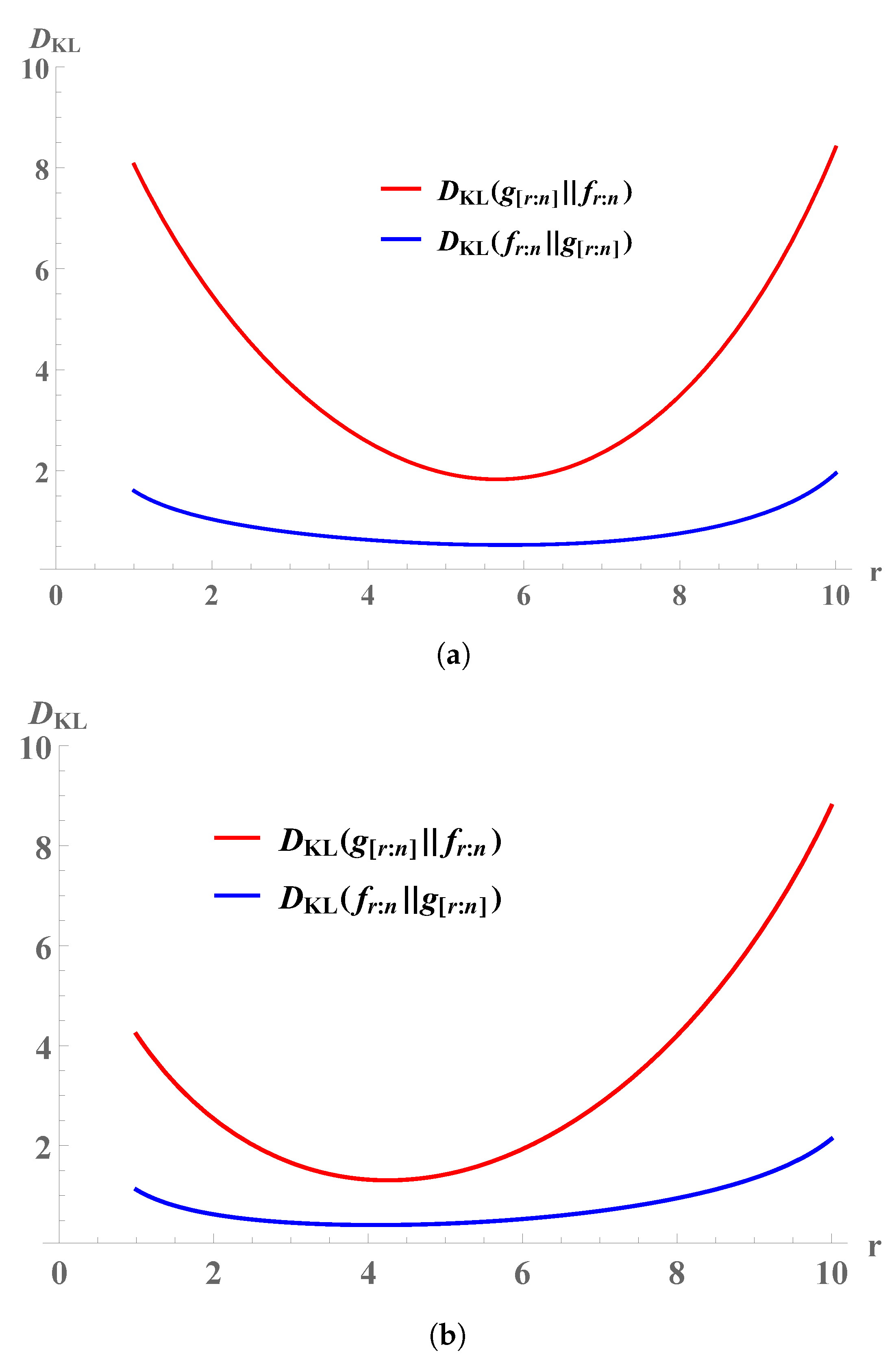
5.2. KL Distance for COSs in HK-FGM3$(a,b)$

The following two Theorems 6 and 7 give the KL distance (defined in (5)) from $Y_{[r:n]}$ to Y and from Y to $Y_{[r:n]}$, respectively, based on HK-FGM3$(a,b).$

Theorem 6.

Let $Y_{[r:n]}$ be the concomitant of rth OS from HK-FGM3$(a,b).$ Then, the KL distance from $Y_{[r:n]}$ to Y is given by

$$\begin{array}{ccc}\hfill D_{KL}(g_{[r:n]}\parallel f_{r:n})& =& ln\beta (r,n-r+1)-{\Omega }_{r,n}+(r-1)\left\{1+\frac{(b+3)}{6}{\Delta }_{r,n}^{}\right\}\hfill \\ & +& (n-r)\left\{1-\frac{(2b+3)}{6}{\Delta }_{r,n}^{}\right\},\hfill \end{array}$$

(22)

where ${\Omega }_{r,n}$ defined in Theorem 5, and ${\Delta }_{r,n}^{}$ is defined via Theorem 1.

Proof. 

By using the PDF of $Y_{[r:n]}$ defined in (11) and the PDF of $Y_{r:n},$ we obtain

$$\begin{array}{ccc}\hfill D_{KL}(g_{[r:n]}\parallel f_{r:n})& =& {\int }_{-\infty }^{\infty }{g}_{[r:n]}\left(y\right)ln\left(\frac{g_{[r:n]}\left(y\right)}{f_{r:n}\left(y\right)}\right)dy\hfill \\ & =& -H\left(Y_{[r:n]}\right)-{\int }_{-\infty }^{\infty }{f}_Y\left(y\right)\left[1+{\Delta }_{r,n}^{}\left\{1+2(b-1)F_Y\left(y\right)-3b{F}_Y^2\left(y\right)\right\}\right]\hfill \\ & \times & ln\left(\frac{1}{\beta (r,n-r+1)}{F}_Y^{r-1}\left(y\right){\overline{F}}_Y^{n-r}\left(y\right)f_Y\left(y\right)\right)dy\hfill \\ & =& ln\beta (r,n-r+1)-H\left(Y_{[r:n]}\right)-(r-1)A-(n-r)B-C,\hfill \end{array}$$

(23)

where

$$A={\int }_{-\infty }^{\infty }{f}_Y\left(y\right)\left[1+{\Delta }_{r,n}^{}\left\{1+2(b-1)F_Y\left(y\right)-3b{F}_Y^2\left(y\right)\right\}\right]ln{F}_Y\left(y\right)dy.$$

Now, taking $u=F_Y\left(y\right),$ we obtain

$$A={\int }_0^1\left[1+{\Delta }_{r,n}^{}\left\{1+2(b-1)u-3b{u}^2\right\}\right]lnudu=-\left\{1+\frac{(b+3)}{6}{\Delta }_{r,n}^{}\right\}.$$

(24)

Similarly, by using the same substitute, we obtain

$$\begin{array}{ccc}\hfill B& =& {\int }_{-\infty }^{\infty }{f}_Y\left(y\right)\left[1+{\Delta }_{r,n}^{}\left\{1+2(b-1)F_Y\left(y\right)-3b{F}_Y^2\left(y\right)\right\}\right]ln{\overline{F}}_Y\left(y\right)dy\hfill \\ & =& {\int }_0^1\left[1+{\Delta }_{r,n}^{}\left\{1+2(b-1)u-3b{u}^2\right\}\right]ln(1-u)du=-\left\{1-\frac{(2b+3)}{6}{\Delta }_{r,n}^{}\right\}.\hfill \end{array}$$

(25)

On the other hand,

$$C=-(1+{\Delta }_{r,n}^{})H\left(Y\right)+{\Delta }_{r,n}^{}\left\{2(b-1){\Phi }_{f_Y}\left(1\right)-3b{\Phi }_{f_Y}\left(2\right)\right\}.$$

(26)

Upon using the value of $H\left(Y_{[r:n]}\right)$ in Theorem 5, and substituting (24–(26) in (23), we obtain (22). The theorem is proved. □

Theorem 7.

Let $Y_{[r:n]}$ be the concomitant of rth OS from HK-FGM3$(a,b).$ Then, the KL distance from Y to $Y_{[r:n]}$ is given by

$$\begin{array}{ccc}\hfill D_{KL}(f_{r:n}\parallel g_{[r:n]})& =& -ln\beta (r,n-r+1)+(r-1)\left\{\psi \left(r\right)-\psi (n+1)\right\}+(n-r)\{\psi (n-r+1)\hfill \\ & -& \psi (n+1)\}-\mathrm{E}\left(ln\left[1+{\Delta }_{r,n}^{}\left\{1+2(b-1)F_Y\left(Y_{[r:n]}\right)-3b{F}_Y^2\left(Y_{[r:n]}\right)\right\}\right]\right),\hfill \end{array}$$

(27)

where $\psi \left(n\right)=\frac{dln\Gamma \left(n\right)}{dn}$ and $\psi (n+1)=\psi \left(n\right)+\frac{1}{n}$.

Proof. We have

$$\begin{array}{ccc}\hfill D_{KL}(f_{r:n}\parallel g_{[r:n]})& =& {\int }_{-\infty }^{\infty }{f}_{r:n}\left(y\right)ln\left(\frac{f_{r:n}\left(y\right)}{g_{[r:n]}}\right)dy\hfill \\ \hfill & =& -H\left(Y_{r:n}\right)-{\int }_{-\infty }^{\infty }{f}_{r:n}\left(y\right)ln\left\{f_Y\left(y\right)\left[1+{\Delta }_{r,n}^{}\left\{1+2(b-1)F_Y\left(y\right)-3b{F}_Y^2\left(y\right)\right\}\right]\right\}dy\hfill \\ \hfill & =& -H\left(Y_{r:n}\right)-{\varphi }_{f_Y}-\mathrm{E}\left(ln\left[1+{\Delta }_{r,n}^{}\left\{1+2(b-1)F_Y\left(Y_{[r:n]}\right)-3b{F}_Y^2\left(Y_{[r:n]}\right)\right\}\right]\right),\hfill \end{array}$$

(28)

where $H\left(Y_{r:n}\right)$ and ${\varphi }_{f_Y}$ defined in [34] as follow

$$H\left(Y_{r:n}\right)=H\left(U_{r:n}\right)-{\varphi }_{f_Y},$$

(29)

where ${\varphi }_{f_Y}={\int }_{-\infty }^{\infty }{f}_{r:n}\left(y\right)ln{f}_Y\left(y\right)dy,$ and $H\left(U_{r:n}\right)$ is the entropy of rth OS from a random sample of size n from uniform $(0,1)$ distribution. An expression for $H\left(U_{r:n}\right)$ is defined as

$$H\left(U_{r:n}\right)=ln\beta (r,n-r+1)-(r-1)[\psi \left(r\right)-\psi (n+1)]-(n-r)[\psi (n-r+1)-\psi (n+1)].$$

Using (28) and (29), we obtain (27). The theorem is proved. □

Figure 1 shows the relation between $D_{KL}(g_{[r:n]}\parallel f_{r:n})$ and $D_{KL}(f_{r:n}\parallel g_{[r:n]})$ based on the HK-FGM3$(a,b)$ copula. We can observe that

1.

Generally, $D_{KL}(g_{[r:n]}\parallel f_{r:n})>D_{KL}(f_{r:n}\parallel g_{[r:n]})$.

2.

Generally, the smallest of $D_{KL}(g_{[r:n]}\parallel f_{r:n})$ and $D_{KL}(f_{r:n}\parallel g_{[r:n]})$ occur near the median, whereas greatest values occur at the extremes.

5.3. FIN for COSs in HK-FGM3$(a,b)$

The next theorem gives the FIN of $Y_{[r:n]},$ based on HK-FGM3$(a,b).$ Moreover, the FIN with exponential marginals is obtained.

Theorem 8.

If $Y_{[r:n]}$ be the concomitant of rth OS from HK-FGM3$(a,b),$ then the FIN of $Y_{[r:n]},$ is given by

$$I_{{}_{f_Y}}\left(Y_{[r:n]}\right)=\mathrm{E}{\left({\left.\frac{\partial ln{g}_{[r:n]}\left(y\right)}{\partial y}\right|}_{y=Y_{[r:n]}}\right)}^2=I_{{}_{f_Y}}\left(Y\right)+{\tau }_{{}_{f_Y}}+4{\phi }_{{}_{f_Y}}+{\delta }_{{}_{f_Y}},$$

where $I_{{}_{f_Y}}\left(Y\right)$ is the FIN of the RV $Y,$ defined by (6),

$$\begin{array}{ccc}\hfill {\tau }_{{}_{f_Y}}& =& {\int }_0^1{\left[\frac{\acute{f_Y}\left(F_Y^{-1}\left(u\right)\right)}{f_Y\left(F_Y^{-1}\left(u\right)\right)}\right]}^2{\Delta }_{r,n}^{}\left\{1+2(b-1)u-3b{u}^2\right\}du,\hfill \\ \hfill {\phi }_{{}_{f_Y}}& =& {\int }_0^1{\Delta }_{r,n}^{}\left\{(b-1)-3b{u}^{}\right\}\acute{f_Y}\left(F_Y^{-1}\left(u\right)\right)du,\hfill \\ \hfill {\delta }_{{}_{f_Y}}& =& {\int }_0^1\frac{{\left[f_Y\left(F_Y^{-1}\left(u\right)\right)\right]}^2{\left[2{\Delta }_{r,n}^{}\left\{(b-1)-3b{u}^{}\right\}\right]}^2}{1+{\Delta }_{r,n}^{}\left\{1+2(b-1)u-3b{u}^2\right\}}du,\hfill \end{array}$$

$\acute{f_Y}\left(y\right)=\frac{\partial f_Y\left(y\right)}{\partial y},$ and $F_Y^{-1}\left(u\right)$ is the quantile function of the DF $F_Y\left(y\right).$

Proof. 

By using (6), the FIN of $Y_{[r:n]}$ can be written as

$$\begin{array}{ccc}\hfill I_{{}_{f_Y}}\left(Y_{[r:n]}\right)& =& \mathrm{E}{\left({\left.\frac{\partial ln{f}_{[r:n]}\left(y\right)}{\partial y}\right|}_{y=Y_{[r:n]}}\right)}^2={\int }_{-\infty }^{\infty }{\left[\frac{\partial ln{f}_{[r:n]}\left(y\right)}{\partial y}\right]}^2{f}_{[r:n]}\left(y\right)dy\hfill \\ & =& {\int }_{-\infty }^{\infty }{\left[\frac{\partial \left\{ln{f}_Y\left(y\right)+ln\left[1+{\Delta }_{r,n}^{}\left\{1+2(b-1)F_Y\left(y\right)-3b{F}_Y^2\left(y\right)\right\}\right]\right\}}{\partial y}\right]}^2\hfill \\ & \times & f_Y\left(y\right)\left[1+{\Delta }_{r,n}^{}\left\{1+2(b-1)F_Y\left(y\right)-3b{F}_Y^2\left(y\right)\right\}\right]dy\hfill \\ & =& {\int }_{-\infty }^{\infty }{\left[\frac{\partial ln{f}_Y\left(y\right)}{\partial y}\right]}^2{f}_Y\left(y\right)dy+{\int }_{-\infty }^{\infty }{\left[\frac{\partial ln{f}_Y\left(y\right)}{\partial y}\right]}^2{\Delta }_{r,n}^{}\hfill \\ & \times & \left\{1+2(b-1)F_Y\left(y\right)-3b{F}_Y^2\left(y\right)\right\}{f}_Y\left(y\right)dy\hfill \\ & +& {\int }_{-\infty }^{\infty }{\left[\frac{\partial ln\left[1+{\Delta }_{r,n}^{}\left\{1+2(b-1)F_Y\left(y\right)-3b{F}_Y^2\left(y\right)\right\}\right]}{\partial y}\right]}^2\hfill \\ & \times & f_Y\left(y\right)\left[1+{\Delta }_{r,n}^{}\left\{1+2(b-1)F_Y\left(y\right)-3b{F}_Y^2\left(y\right)\right\}\right]dy+2{\int }_{-\infty }^{\infty }\frac{\partial ln{f}_Y\left(y\right)}{\partial y}\hfill \\ & \times & \frac{\partial ln\left[1+{\Delta }_{r,n}^{}\left\{1+2(b-1)F_Y\left(y\right)-3b{F}_Y^2\left(y\right)\right\}\right]}{\partial y}\hfill \\ & \times & f_Y\left(y\right)\left[1+{\Delta }_{r,n}^{}\left\{1+2(b-1)F_Y\left(y\right)-3b{F}_Y^2\left(y\right)\right\}\right]dy\hfill \\ & =& I_{{}_{f_Y}}\left(Y\right)+{\int }_{-\infty }^{\infty }{\left[\frac{\partial ln{f}_Y\left(y\right)}{\partial y}\right]}^2{\Delta }_{r,n}^{}\left\{1+2(b-1)F_Y\left(y\right)-3b{F}_Y^2\left(y\right)\right\}{f}_Y\left(y\right)dy\hfill \\ & +& {\int }_{-\infty }^{\infty }\frac{f_Y^3\left(y\right){\left[2{\Delta }_{r,n}^{}\left\{(b-1)-3b{F}_Y\left(y\right)\right\}\right]}^2}{1+{\Delta }_{r,n}^{}\left\{1+2(b-1)F_Y\left(y\right)-3b{F}_Y^2\left(y\right)\right\}}dy\hfill \\ & +& 4{\int }_{-\infty }^{\infty }{\Delta }_{r,n}^{}\left\{(b-1)-3b{F}_Y\left(y\right)\right\}{\acute{f}}_Y\left(y\right)f_Y\left(y\right)dy.\hfill \end{array}$$

(30)

Upon using the transformation $u=F_Y\left(y\right)$ in the three integrations on the right of (30) and simplifying the result, we obtain the required result. □

Example 1.

Suppose that X and Y have exponential CDFs, i.e., $X\sim exp\left({\theta }^{★}\right)$ and Y $\sim exp\left(\theta \right)$ with JPDF (1); by using Theorem 8, we obtain

$$\begin{array}{ccc}\hfill I_{{}_{f_Y}}\left(Y\right)& =& {\int }_0^{\infty }{\left[\frac{\partial ln\left(\theta e^{-\theta y}\right)}{\partial y}\right]}^2\left(\theta e^{-\theta y}\right)dy={\theta }^2,\hfill \\ \hfill {\tau }_{{}_{f_Y}}& =& {\int }_0^{\infty }{\left[\frac{\partial ln\left(\theta e^{-\theta y}\right)}{\partial y}\right]}^2\theta e^{-\theta y}\left[{\Delta }_{r,n}^{}\{1+2(b-1)(1-e^{-\theta y})-3b{(1-e^{-\theta y})}^2\}\right]dy\hfill \\ & =& {\theta }^2\left({\Delta }_{r,n}^{}\{1+\frac{1}{2}\left(2(b-1)\right)-\frac{1}{3}\left(3b\right)\}\right)=0,\hfill \end{array}$$

and

$${\phi }_{{}_{f_Y}}={\int }_0^{\infty }\left[{\Delta }_{r,n}^{}\{2(b-1)-6b{(1-e^{-\theta y})}^{}\}\right](-{\theta }^2\left(\theta e^{-2\theta y}\right))dy={\Delta }_{r,n}^{}{\theta }^2.$$

Thus, the FIN of $Y_{[r:n]}$ is given by $I_{{}_{f_Y}}\left(Y_{[r:n]}\right)={\theta }^2+2{\theta }^2{\Delta }_{r,n}^{}+{\delta }_{{}_{f_Y}},$ where

$${\delta }_{{}_{f_Y}}={\theta }^3{\int }_0^{\infty }\frac{e^{-3\theta y}{\left[{\Delta }_{r,n}^{}\{2(b-1)-6b{(1-e^{-\theta y})}^{}\}\right]}^2}{1+{\Delta }_{r,n}^{}\left\{1+2(b-1)(1-e^{-\theta y})-3b{(1-e^{-\theta y})}^2\right\}}dy.$$

(31)

The integration (31) can be numerically evaluated by Mathematica Ver. 12.

5.4. CPI between $Y_{[r:n]}$ and Y Based on HK-FGM3$(a,b)$

If $Y_{[r:n]}$ is the concomitant of rth OS from HK-FGM3$(a,b)$ then the CPI (defined in (7)) between $G_{[r:n]}\left(y\right)$ and $F_Y\left(y\right),$ is given by

$$\begin{array}{ccc}\hfill I(G_{[r:n]},F_Y)& =& -{\int }_{-\infty }^{\infty }{F}_Y\left(y\right)\left[1+{\Delta }_{r,n}\left\{1+(b-1)F_Y\left(y\right)-b{F}_Y^2\left(y\right)\right\}\right]ln{F}_Y\left(y\right)dy\hfill \\ & =& \left(1+{\Delta }_{r,n}\right)\tilde{H}\left(Y\right)+{\Delta }_{r,n}\left\{\frac{(b-1)}{2}\tilde{H}\left(Y_{2:2}\right)-\frac{b}{3}\tilde{H}\left(Y_{3:3}\right)\right\},\hfill \end{array}$$

(32)

where $\tilde{H}\left(Y_{p+1:p+1}\right)=-{\int }_{-\infty }^{\infty }(p+1)F_Y^{(p+1)}\left(y\right)ln{F}_Y\left(y\right)dy,p=1,2,$ is the cumulative entropy of the RV $Y_{p+1:p+1}.$ When we put $b=0$ in (32), we obtain the result of [35].

Example 2.

Suppose that X and Y have exponential DFs, with means $\frac{1}{{\theta }^{★}}$ and $\frac{1}{\theta }$, respectively, with JPDF of HK-FGM3$(a,b:{\theta }^{★},1;\theta ,1)$. Clearly, we have

$$\begin{array}{ccc}\hfill I(G_{[r:n]},F_Y)& =& \left(1+{\Delta }_{r,n}\right){\int }_0^{\infty }-(1-exp(-\theta y))ln\left((1-exp(-\theta y))\right)dy\hfill \\ & +& (b-1){\Delta }_{r,n}{\int }_0^{\infty }-{(1-exp(-\theta y))}^{2}ln((1-exp(-\theta y))dy\hfill \\ & -& b{\Delta }_{r,n}{\int }_0^{\infty }-{(1-exp(-\theta y))}^{3}ln((1-exp(-\theta y))dy\hfill \\ & =& \left(1+{\Delta }_{r,n}\right)\frac{{\pi }^2-6}{6\theta }+(b-1){\Delta }_{r,n}\frac{2{\pi }^2-15}{12\theta }-b{\Delta }_{r,n}\frac{6{\pi }^2-49}{36\theta }.\hfill \end{array}$$

Table 3. CPI between $Y_{[r:n]}$ and Y based on HK-FGM3$(a,b:{\theta }^{★},1;\theta ,1)$ copula.

		$\mathit{b}\mathbf{=}\mathbf{0.9}$		$\mathit{b}\mathbf{=}\mathbf{-}\mathbf{1}$		$\mathit{b}\mathbf{=}\mathbf{2}$		$\mathit{b}\mathbf{=}\mathbf{-}\mathbf{3}$
$\mathit{n}$	$\mathit{r}$	$\mathit{a}=-\mathbf{0}.\mathbf{2}$	$\mathit{a}=\mathbf{0}.\mathbf{2}$	$\mathit{a}=-\mathbf{0}.\mathbf{75}$	$\mathit{a}=-\mathbf{0}.\mathbf{25}$	$\mathit{a}=-\mathbf{0}.\mathbf{1}$	$\mathit{a}=\mathbf{0}.\mathbf{1}$	$\mathit{a}=-\mathbf{0}.\mathbf{2}$	$\mathit{a}=\mathbf{0}.\mathbf{2}$
3	1	0.59733	0.69253	0.61368	0.63452	0.60243	0.68743	0.64327	0.64660
3	2	0.63863	0.65123	0.65535	0.64841	0.63549	0.65438	0.63993	0.64993
3	3	0.69883	0.59103	0.66577	0.65188	0.69688	0.59299	0.65160	0.63827
5	1	0.58627	0.70360	0.59533	0.62840	0.59546	0.69441	0.64652	0.64335
5	2	0.60660	0.68327	0.63501	0.64163	0.60671	0.68316	0.63859	0.65128
5	3	0.63593	0.65393	0.65982	0.64989	0.63144	0.65843	0.63779	0.65208
5	4	0.67427	0.61560	0.66974	0.65320	0.66967	0.62020	0.64414	0.64573
5	5	0.72160	0.56827	0.66478	0.65155	0.72139	0.56848	0.65763	0.63224
7	1	0.58193	0.70793	0.58417	0.62468	0.59378	0.69609	0.64910	0.64077
7	2	0.59418	0.69568	0.61889	0.63625	0.59771	0.69216	0.64077	0.64910
7	3	0.61168	0.67818	0.64493	0.64493	0.60952	0.68035	0.63660	0.65327
7	4	0.63443	0.65543	0.66230	0.65072	0.62919	0.66068	0.63660	0.65327
7	5	0.66243	0.62743	0.67098	0.65362	0.65674	0.63313	0.64077	0.64910
7	6	0.69568	0.59418	0.67098	0.65362	0.69216	0.59771	0.64910	0.64077
7	7	0.73418	0.55568	0.66230	0.65072	0.73544	0.55443	0.66160	0.62827
9	1	0.57977	0.71010	0.57675	0.62221	0.59342	0.69645	0.65100	0.63887
9	2	0.58804	0.70183	0.60706	0.63231	0.59428	0.69559	0.64312	0.64675
9	3	0.59975	0.69012	0.63168	0.64052	0.60029	0.68958	0.63796	0.65190
9	4	0.61490	0.67497	0.65062	0.64683	0.61145	0.67842	0.63554	0.65433
9	5	0.63348	0.65639	0.66387	0.65125	0.62776	0.66211	0.63584	0.65403
9	6	0.65550	0.63437	0.67145	0.65377	0.64923	0.64064	0.63887	0.65100
9	7	0.68095	0.60892	0.67334	0.65440	0.67584	0.61403	0.64463	0.64524
9	8	0.70984	0.58003	0.66956	0.65314	0.70761	0.58226	0.65312	0.63675
9	9	0.74217	0.54770	0.66009	0.64999	0.74453	0.54534	0.66433	0.62554

displays the CPI between $Y_{[r:n]}$ and Y based on HK-FGM3$(a,b:{\theta }^{★},1;\theta ,1)$ copula. The following properties can be extracted:

• In most cases, with fixed $n,$ the value of $I(G_{[r:n]},F_Y)$ increases as r increase, when a is negative.
• In most cases, with fixed $n,$ the value of $I(G_{[r:n]},F_Y)$ decreases as r increase, when a is positive.

6. Concluding Remarks

Even though HK-FGM3$(a,b)$’s efficiency based on the correlation level is comparable to that of other generalizations of FGM (such as HK-FGM DFs), its flexibility and usability enable it to exceed many other generalizations of FGM. This benefit led to the current paper’s PDFs always being linear fusions of other simpler distributions. We identified a number of distributional features of the COSs based on HK-FGM3$(a,b)$. Simple deductions were also made on the relationships between PDFs, HRF, MGFs, and moments of concomitants. Additionally, based on HK-FGM3$(a,b)$, the asymptotic behavior of the concomitant rank of OSs was determined. The Shannon entropy, KL distance, FIN, and CPI for the COSs are some information measures that have been developed and explored.

Two aspects are considered while discussing the possibility of additional study. We can first apply the research’s conclusions to extropy (dual of entropy) and the related measures of information. The second target research project in the future is to estimate these measures using traditional and Bayesian approaches. In the literature, Bayesian approaches received significant attention, as seen by Ahmadi et al. [36].

References

1. Ghosh, S.; Sheppard, L.W.; Holder, M.T.; Loecke, T.D.; Reid, P.C.; Bever, J.D.; Reuman, D.C. Copulas and their potential for ecology. Adv. Ecol. Res. 2020, 62, 409–468. [Google Scholar]
2. Ota, S.; Kimura, M. Effective estimation algorithm for parameters of multivariate Farlie-Gumbel-Morgenstern copula. Jpn. J. Stat. Data Sci. 2021, 4, 1049–1078. [Google Scholar] [CrossRef]
3. Shrahili, M.; Alotaibi, N. A new parametric life family of distributions: Properties, copula and modeling failure and service times. Symmetry 2020, 12, 1462. [Google Scholar] [CrossRef]
4. Shih, J.H.; Konno, Y.; Chang, Y.T.; Emura, T. Copula based estimation methods for a common mean vector for bivariate meta-analyses. Symmetry 2022, 14, 186. [Google Scholar] [CrossRef]
5. Takeuchi, T.T. Constructing a bivariate distribution function with given marginals and correlation: Application to the galaxy luminosity function. Mon. Not. R. Astron. Soc. 2010, 406, 1830–1840. [Google Scholar] [CrossRef] [Green Version]
6. Huang, J.S.; Kotz, S. Correlation structure in iterated Farlie-Gumbel-Morgenstern distributions. Biometrika 1984, 71, 633–636. [Google Scholar]
7. Huang, J.S.; Kotz, S. Modifications of the Farlie-Gumbel-Morgenstern distributions. A tough hill to climb. Metrika 1999, 49, 135–145. [Google Scholar] [CrossRef]
8. Barakat, H.M.; Alawady, M.A.; Husseiny, I.A.; Abd Elgawad, M.A. A more flexible counterpart of Huang-Kotz’s copula-type. C. R. Acad. Bulg. Sci. 2022, 75, 952–958. [Google Scholar] [CrossRef]
9. Barakat, H.M.; Alawady, M.A.; Abd Elgawad, M.A. Correction to the paper: A new extension of the FGM Copula with an application in reliability by Rasha Ebaid, Walid Elbadawy, Essam Ahmed and Abdalla Abdelghaly. Commun. Stat.-Theory Methods 2021, 1–2. [Google Scholar] [CrossRef]
10. Ebaid, R.; Elbadawy, W.; Ahmed, E.; Abdelghaly, A. A new extension of the FGM copula with an application in reliability. Commun. Stat.-Theory Methods 2022, 51, 2953–2961. [Google Scholar] [CrossRef]
11. Gupta, R.D.; Kundu, D. Generalized exponential distributions. Aust. N. Z. J. Stat. 1999, 41, 173–188. [Google Scholar] [CrossRef]
12. David, H.A.; Nagaraja, H.N. Concomitants of Order Statistics. In Handbook of Statistics; Balakrishnan, N., Rao, C.R., Eds.; Elsevier: Amsterdam, Netherlands, 1998; Volume 16, pp. 487–513. [Google Scholar]
13. Tahmasebi, S.; Jafari, A.A. Concomitants of order statistics and record values from Morgenstern type bivariate-generalized exponential distribution. Bull. Malays. Math. Sci. Soc. 2015, 38, 1411–1423. [Google Scholar] [CrossRef]
14. Scaria, J.; Nair, N.U. On concomitants of order statistics from Morgenstern family. Biom. J. J. Math. Methods Biosci. 2015, 1999, 41–483. [Google Scholar] [CrossRef]
15. Shannon, C.E. A mathematical theory of communication. Bell Syst. Tech. J. 1948, 27, 379–423. [Google Scholar] [CrossRef] [Green Version]
16. Bormashenko, E. Entropy, Information, and Symmetry: Ordered is Symmetrical. Entropy 2019, 22, 11. [Google Scholar] [CrossRef] [PubMed] [Green Version]
17. Jiang, X.; Song, T.; Katayama, K. Maximum-entropy-model-enabled complexity reduction algorithm in modern video coding standards. Symmetry 2020, 12, 113. [Google Scholar] [CrossRef] [Green Version]
18. Rao, M.; Chen, Y.; Vemuri, B.C.; Wang, F. Cumulative residual entropy: A new measure of information. IEEE Trans. Inf. Theory 2004, 50, 1220–1228. [Google Scholar] [CrossRef]
19. Kullback, S.; Leibler, R.A. On information and sufficiency. Ann. Math. Stat. 1951, 22, 79–86. [Google Scholar] [CrossRef]
20. Contreras-Reyes, J.E. An asymptotic test for bimodality using the Kullback–Leibler divergence. Symmetry 2020, 12, 1013. [Google Scholar] [CrossRef]
21. Kerridge, D.F. Inaccuracy and inference. J. R. Stat. Soc. 1961, 23, 184–194. [Google Scholar] [CrossRef]
22. Rao, B.R. On an analogue of Cramer-Rao inequality. Skand. Actuar. Tidskr 1958, 41, 57–64. [Google Scholar] [CrossRef]
23. Frieden, B.R.; Gatenby, R.A. (Eds.) Exploratory Data Analysis Using Fisher Information; Springer: London, UK, 2007. [Google Scholar]
24. Papaioannou, T.; Ferentinos, K. On two forms of Fisher’s measure of information. Commun. Stat.-Theory Methods 2005, 34, 1461–1470. [Google Scholar] [CrossRef]
25. Thapliyal, R.; Taneja, H.C. A measure of inaccuracy in order statistics. J. Stat. Theory Appl. 2013, 12, 200–207. [Google Scholar] [CrossRef] [Green Version]
26. Thapliyal, R.; Taneja, H.C. On residual inaccuracy of order statistics. Stat. Probab. Lett. 2015, 97, 125–131. [Google Scholar] [CrossRef]
27. Abd Elgawad, M.A.; Alawady, M.A.; Barakat, H.M.; Xiong, S. Concomitants of generalized order statistics from Huang-Kotz Farlie-Gumbel-Morgenstern bivariate distribution: Some information measures. Bull. Malays. Math. Sci. Soc. 2020, 43, 2627–2645. [Google Scholar] [CrossRef]
28. Thapliyal, R.; Taneja, H.C. Dynamic cumulative residual and past inaccuracy measures. J. Stat. Theory Appl. 2015, 14, 399–412. [Google Scholar]
29. Galambos, J. The Asymptotic Theory of Extreme Order Statistics, 2nd ed.; Robert E. Krieger Publishing Company: Malabar, FL, USA, 1987. [Google Scholar]
30. David, H.A.; O’Connell, M.J.; Yang, S.S. Distribution and expected value of the rank of a concomitant and an order statistic. Ann. Stat. 1977, 5, 216–223. [Google Scholar] [CrossRef]
31. Barakat, H.M.; El-Shandidy, M.A. Computing the distribution and expected value of the concomitant rank order statistics. Commun. Stat.-Theory Methods 2004, 33, 2575–2594. [Google Scholar] [CrossRef]
32. Barakat, H.M.; Nigm, E.M.; Harpy, M.H. Limit theorems of order statistics and record values from the gamma and Kumaraswamy-generated-distributions. Bull. Malays. Math. Sci. Soc. 2017, 40, 1055–1069. [Google Scholar] [CrossRef]
33. Barakat, H.M.; Alawady, M.A.; Husseiny, I.A.; Mansour, G.M. Sarmanov family of bivariate distributions: Statistical properties concomitants of order statistics information measures. Bull. Malays. Math. Sci. Soc. 2022, 45, 49–83. [Google Scholar] [CrossRef]
34. Ebrahimi, N.; Soofi, E.S.; Zahedi, H. Information properties of order statistics and spacings. IEEE Trans. Inf. Theory 2004, 50, 177–183. [Google Scholar] [CrossRef]
35. Daneshi, S.; Nezakati, A.; Tahmasebi, S. Measures of inaccuracy for concomitants of generalized order statistics. In Proceedings of the 14th Iranian Statistics Conference, Shahrood University of Technology, Shahrood, Iran, 25–27 August 2018; pp. 154–161. [Google Scholar]
36. Ahmadi, K.; Akbari, M.; Raqab, M.Z. Objective Bayesian estimation for the differential entropy measure under generalized half-normal distribution. Bull. Malays. Math. Sci. Soc. 2023, 46, 39. [Google Scholar] [CrossRef] [PubMed]
Figure 1. Representation of the  D K L ( g [ r : n ] f r : n )  and  D K L ( f r : n g [ r : n ] )  arising from  Y [ r : 10 ] .  (a a = 0.2 , b = 0.9 , n = 10 ; (b a = 0.5 , b = 0.9 , n = 10 .
Symmetry 15 01257 g001