Abstract
With the enhanced interoperability of information among vehicles, the demand for collaborative sharing among vehicles increases. Based on blockchain, the classical consensus algorithms in collaborative IoV (Internet of Vehicle), such as PoW (Proof of Work), PoS (Proof of Stake), and DPoS (Delegated Proof of Stake), only consider the node features, which is hard to adapt to the immediacy and flexibility of vehicles. On the other hand, classical consensus algorithms often require mass computing, which undoubtedly increases the communication overhead, resulting in the inability to achieve collaborative IoV under asymmetric networks. Therefore, proposing a low failure rate consensus algorithm that takes into account running time and energy consumption becomes a major challenge in IoV applications. This paper proposes an AI-enabled consensus algorithm with vehicle features, combining vehicle-based metrics and neural networks. First, we introduce vehicle-based metrics such as vehicle online time, performance, and behavior. Then, we propose an integral model and a hierarchical classification method, which combine with a BP neural network to obtain the optimal solution for interconnection. Among them, we also use Informer to predict the future online duration of vehicles, which effectively solves the situation that the primary node vehicle drops off in collaborative IoV. Finally, the experimentations show that the vehicle-based metrics eliminate the problem of the primary node vehicle being offline, which realizes the collaborative IoV considering vehicle features. Meanwhile, it reduces the vehicle network system delay and energy consumption.
1. Introduction
With the popularity of vehicles, people pay more and more attention to the driving experience. Nowadays, drivers are not only satisfied with the location information services provided by vehicles, but also with the safety, effectiveness of information sharing, and energy saving. Therefore, facing the huge number of vehicles and a rapidly changing traffic environment, it is a crucial technical issue to reduce the possibility of communication errors and system delays [1]. As we all know, more and more nodes of collaborative networks among vehicles are constantly upgraded and updated. Vehicles share pictures, videos, and control signaling collected by themselves, such as road traffic data, vehicle location data, driving habits data, and vehicle-to-vehicle interaction data [2], so that vehicles can grasp the surrounding environment information more quickly, to comprehensively consider and judge their own driving state. In order to better realize information sharing and interaction between vehicles, collaborative vehicle networking emerged [3,4,5].
In collaborative vehicle networking, there are many problems in data sharing. First of all, for the stability of the vehicle networking system, the traditional centralized network architecture has problems, such as single point of failure and privacy disclosure [6]. Therefore, considering the distributed characteristics of collaborative vehicle networking, many related studies have applied blockchain to it. Technologies such as distributed ledger, consensus mechanism, and smart contract in blockchain can effectively solve data security and trust problems in the process of data sharing [7]. However, traditional blockchains were originally born in the financial industry. Moreover, many papers directly apply blockchain to collaborative vehicle networking [8,9], without involving the inherent attributes of vehicles and drivers, which is easy to cause the selected “primary node vehicle” to go offline at any time, or the driver to interrupt the interconnection. Therefore, the main node vehicle dropout rate is the first problem to be solved in this paper. Second, for information sharing to be effective, vehicles must make decisions within a relatively short delay after data collection. However, the classical consensus algorithm usually requires a large amount of computation or frequent communication [10,11], which will lead to communication delay and hinder the interconnection of collaborative vehicle networks. Communication delay is the second problem to be solved in this paper. Further, it is common for researchers to reduce the drop-off rate and system latency at the primary node through frequent communication. This undoubtedly greatly increases the energy cost of the entire system. Reducing energy consumption is the third problem to be addressed in this paper.
Focusing on the above three aspects of the problem, based on the blockchain consensus mechanism, this paper proposes a vehicle-based consensus algorithm. It uses an objective vehicle-based rating system instead of subjective voting to assess whether there is a malicious association in the historical behavior of nodes. The method verifies whether nodes have a negative impact on the blockchain based on points accumulated from the vehicle’s historical behavior. Therefore, it reduces the probability that the node is a Byzantine node. The experimental results show that our algorithm greatly reduces the possibility of interconnection disruption and effectively reduces transaction latency. Our approach ensures the safety, stability, and effectiveness of collaborative vehicle networking while saving energy costs significantly.
The contributions of this paper are as follows:
- Combine the principle of blockchain and consider the indicators of the driver’s driving experience to build an integral model and classification model suitable for collaborative vehicle networking information sharing.
- By improving the consensus algorithm, an energy-saving AI-Enabled Proof of Vehicle (AI-PoV) consensus algorithm is proposed to reduce the failure rate and system delay.
- Our experiment verifies the effectiveness of the AI-PoV algorithm.
The rest of this article is organized as follows. Section 2 introduces the research content of related work in detail. Section 3 introduces the system model and index of this paper. Section 4 describes our AI-PoV algorithm. In Section 5, experimental results are given and compared with the other three methods. Finally, Section 6 summarizes the full text.
2. Related Works
Data security has always been an important research objective of the Internet of Things. Ref. [12] discussed the use of machine learning in network security research in their paper, pointing out that while we use machine learning to maintain network security, attackers are attempting to use machine learning to launch network attacks. Therefore, the development of new network security technologies is imminent. Ref. [13] addressed the issue of poor stability of intelligent systems using the radial basis function neural network model, improving the anti-jamming ability of vehicles and protecting critical vehicle data. Similarly, [14] found that autonomous driving technology can effectively improve the safety performance of vehicles. They proposed a better target recognition algorithm by combining it with vehicle perception technology. Ref. [15] proposed a data collection framework for creating fused datasets that can distinguish harmful data from unmanned remote-controlled vehicles to prevent damage caused by intrusion.
Much research has optimized the high delay caused by the asymmetric network structure in the vehicle network. Ref. [16] designs a computing resource trading strategy based on Blockchain-as-a-Service, which evaluates participants’ task delays, energy costs, transaction prices, and participants’ reputation scores, and then allocates tasks to solve the problem of asymmetry between edge and terminal computing resources and capabilities. Ref. [17], based on deep Q network to allocate resources according to the request frequency of content and the network status of nodes, the content cache and request routing of cross-layer cooperation are optimized, which ensures low-latency network communication in asymmetric IoV. Ref. [18] regards edge devices as symmetrical P2P (peer-to-peer) networks, and proposes an efficient and fault-tolerant computing offload strategy, which provides the optimal node to interact with the vehicle and reduces the task completion delay. These studies address the communication delay problem in asymmetric vehicular networks by optimizing the task allocation between edge devices or by facilitating collaborative computation among edge devices. However, they overlook the communication issues between terminal devices. In other words, these studies only consider the communication direction from edge to edge or from edge to terminal, but neglect the direction from terminal to terminal. Especially, the application of blockchain technology in IoT has enormous potential, and communication between vehicles in a blockchain environment is essential.
Much research on blockchain in IoV revolves around traditional consensus algorithms or improved consensus algorithms. PoW (Proof of Work), is the most classic consensus algorithm based on their computing power, in which the node that solves the problem the fastest will obtain the right, and the system automatically generates the reward [19]. PoS (Proof of Stake) allows the block creator to act as the verifier, using proof of equity instead of PoW’s proof of computing power, with billing rights obtained by the node with the highest equity. Equity is used as a vote to elect bookkeepers, and then bookkeepers take turns keeping accounts [20]. Based on PoS, DPoS (Delegated Proof of Stake) professionalizes the role of bookkeepers. It first selects bookkeepers with equity as votes and then takes turns among bookkeepers to keep accounts [21]. These traditional consensus algorithms were originally proposed to be applied in the financial field. However, the vehicle computing resources and energy in the Internet of Vehicles are limited [22], and the security requirements are high, so these traditional consensus algorithms do not meet the requirements of the vehicle network and cannot be directly applied.
Many improved consensus algorithms exist in IoV. Ref. [23] proposes a decentralized trust management system, which uses Bayesian inference models to evaluate the reliability of the information received from neighboring vehicles. It adopts the joint consensus mechanism of PoW and PoS. The higher the share, the easier it is to find the hash value. Ref. [24] proposed a trust management model based on blockchain, combined with a conditional privacy protection announcement scheme for IoV. It uses a hybrid consensus algorithm based on PoW and PBFT (Practical Byzantine Fault Tolerance). BTCPS (blockchain-based TM with conditional privacy-preserving scheme) selects miners by PoW and uses PBFT to reach a consensus. Many approaches were chosen for several other tasks. Ref. [25] proposes an enhanced DPoS consensus solution with a two-stage soft security solution to ensure the safety of vehicle data sharing and to select safe miners based on reputation. Ref. [26] proposed a T-PBFT algorithm based on the EigenTrust model, which evaluated the trust value of nodes through the transactions between nodes, and then selected nodes with high trust value in the network to establish a consensus group. It optimizes the PBFT consensus algorithm to reduce the number of nodes required by PBFT consensus by grouping, thus reducing message complexity and increasing throughput. Although these studies have improved traditional consensus algorithms to make them more suitable for vehicular networks, they overlook the unique characteristics of vehicles themselves. Some vehicle features reflect the quality of nodes to a great extent. For example, vehicles with good communication conditions tend to have high communication efficiency, and vehicles that violate traffic rules less often tend to better obey broadcast rules. Our study extracts the characteristics of vehicles themselves and implements a vehicle-based consensus algorithm, which is highly suited to IoV.
We have summarized the related works in a table, as shown in Table 1.

Table 1.
Related work summary.
3. System Models
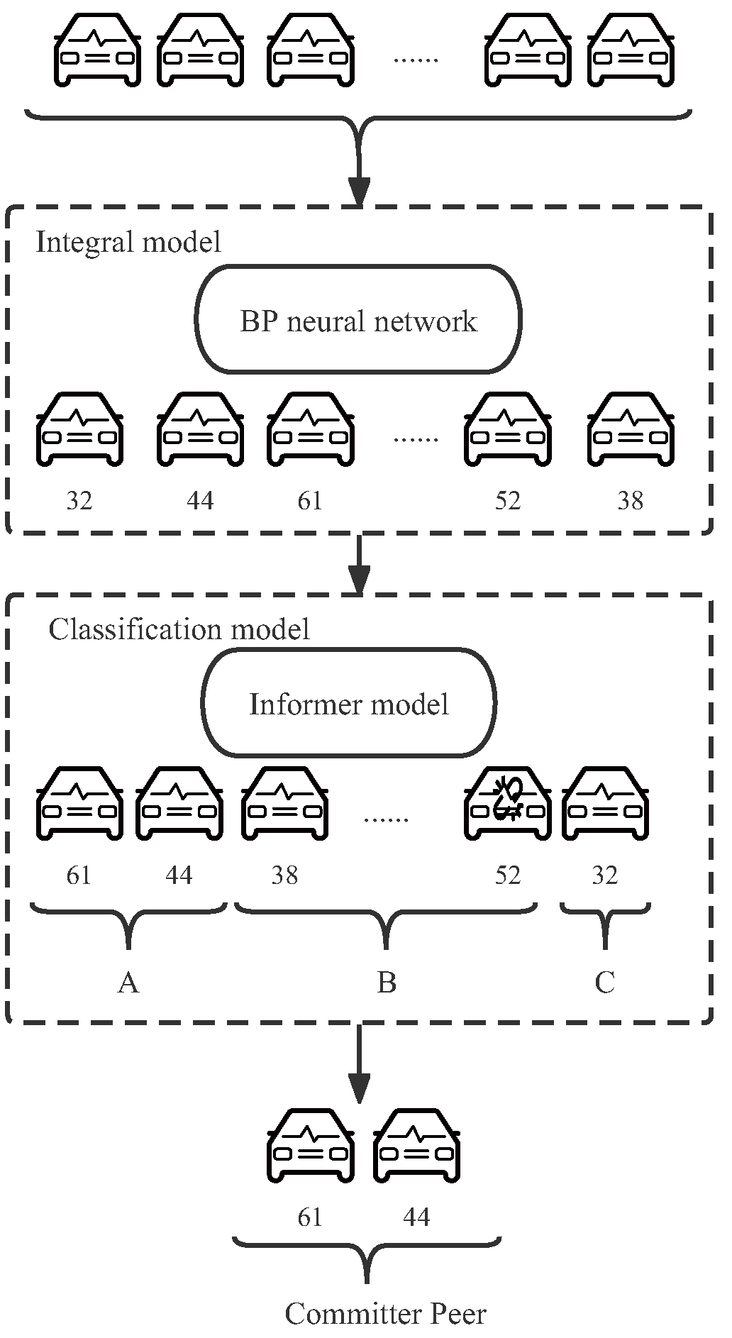
In the consensus algorithm, selecting primary nodes is an important problem. In this section, we list a series of models we used to select a primary node, including the Integral model and the Classification model. The overall execution flow of the system model is shown in Figure 1. In the context of a public chain consisting of blockchain nodes for each vehicle, the vehicles are scored by the Integral model, with the number of each vehicle representing its score. Vehicles are then further selected through the Classification model, and it is worth noting that offline vehicles are demoted. Eventually, vehicles eligible to participate in bookkeeping will be polled and become master nodes.
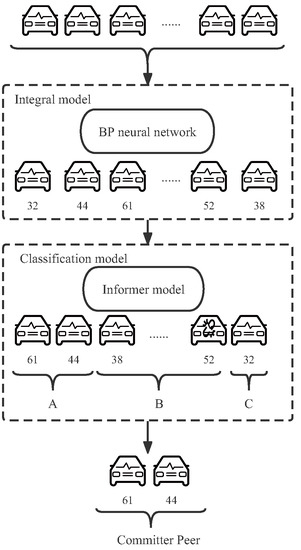
Figure 1.
The flowchart of selecting the primary node.
3.1. Integral Model
In this paper, we use the integral model to evaluate the performance of vehicles in the consensus process [27]. Vehicles with higher scores are more likely to get the accounting right [28]. The vehicle score is mainly affected by the following four types of features: vehicle attribute, vehicle wealth, vehicle integrity, and vehicle performance. Each primary indicator is also subdivided into sub-indicators, with a total of 10 reference criteria that together determine the node’s score, as shown in Table 2.

Table 2.
Integral model index description.
The vehicle attribute is the relevant parameter information of the vehicle itself, including the running frequency of the vehicle memory and the running power. The higher the frequency of the vehicle, the better the performance; the lower the power of the vehicle, the lower the energy consumption. So the frequency is positively correlated with the integral, and the power is negatively correlated with the integral.
Vehicle wealth is based on the index generated by the PoS algorithm, specifically according to the currency age of the vehicle, the older the currency is, the more you do not want the blockchain system to be attacked, so it is positively related to the score.
Vehicle integrity is related to the performance of vehicles after several rounds of consensus, including the number of forked blocks, the number of error/invalid or wrong blocks, traffic offense points, and last round integral. Providing forked blocks, providing error/invalid, or wrong blocks represents that the vehicle is providing wrong information; the more times, the more likely they are malicious nodes. Traffic offense points reflect the extent to which drivers abide by the rules, and vehicles that do not abide by the rules can easily become malicious nodes. So the first two secondary indicators are positively correlated with credits. the last two items are negatively related to the score.
Vehicle performance is related to the network, including the duration of participation in the network, network delay, and vehicle offline times. These indicators reflect the communication efficiency of the vehicle. So the first secondary index is positively related to the integral, and the latter two are negatively related to the integral. The vehicle attribute index aims to select vehicles with high computational efficiency, vehicle wealth and vehicle integrity aim to improve the fault tolerance rate of communication, and vehicle performance aims to select vehicles with low delay communication.
These indicators can guide us to choose a terminal with high efficiency, high fault tolerance, and low delay. In asymmetric IoV, terminals with good performance can share some tasks of the server, thus reducing the negative impact brought by asymmetric network structure. We use these metrics to score the vehicle by training a model through a BP neural network, which is described in detail in Section 4.1.
3.2. Classification Model
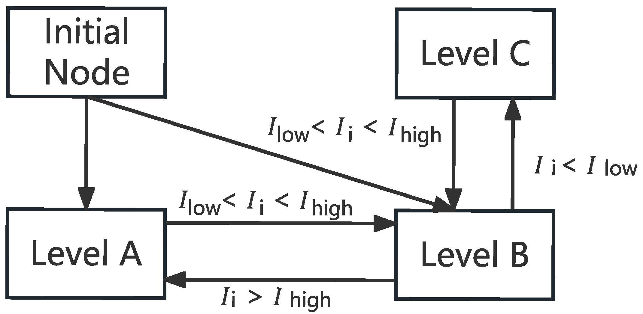
According to the previous subsection, we obtain a training model. The vehicle score can be obtained by inputting various index parameters. In this subsection, based on the vehicle scores derived from the model in Section 3.1, we use the classification model to further classify the vehicles so as to select the vehicles suitable as master nodes. Vehicle levels are first divided into three levels: A, B, and C. is defined as the integral of a vehicle and is derived from the Integral model. Two constants, and , are used to classify the vehicle to different levels. If > , the node is assigned to Level A; If < < , the node is assigned to Level B. If the < , nodes are classified as Level C. This process is shown in Figure 2.
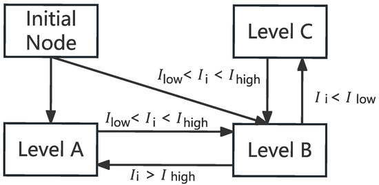
Figure 2.
Classification conditions.
Vehicles at different levels have different permissions, among which vehicles at Level A can obtain the bookkeeping right by polling; In Level B, vehicles have alternate bookkeeping rights. They can be used as excellent terminals to undertake some computing tasks, which is more advantageous than asymmetric centralized communication structure. Although there are no bookkeeping rights can still store information and verify other consensus vehicle bookkeeping is correct, as long as the active participation in the consensus is likely to rise to A; Level C vehicles are most likely Byzantine vehicles, which deprived them of the right to participate in the consensus. This practice can greatly improve the enthusiasm of vehicles, prevent Byzantine vehicles from obtaining accounting rights caused by bad effects, and even prohibit their participation in the consensus.
In the initial stage, the vehicles have not gone through the consensus process, so there will be no negative score. Whether they can enter Level A is largely determined by vehicle performance and network conditions. Therefore, most vehicles are in Level A or Level B, and there may even be no vehicles entering Level A, so the accounting consensus vehicles are temporarily selected from Level B. After several rounds of consensus, the number of points of vehicles with good performance will increase and be upgraded, while the number of points of vehicles with poor performance will decrease and be downgraded.
For Level A vehicles, we want them to be online, so we need to predict their online status. This can further improve the fault tolerance rate of communication. This is a time series prediction problem because we are applying it to vehicles. The online status of a vehicle is mainly affected by the following features: time, public transport conditions, air temperature, rainfall, and vehicle life as shown in Table 3.

Table 3.
Vehicle online status evaluation indicators description.
Time is the period for collecting relevant information, and time series are used to predict the online status of vehicles. The public transportation situation is a rating of the public transportation in the city where the vehicle is located. The convenience of public transportation has a significant impact on the use of vehicles. When local public transportation can meet people’s travel needs, they will reduce the use of vehicles. Climate is also an important factor affecting vehicle use. When the temperature is too high or too low, or when it is raining, people tend to choose vehicles for travel due to comfort considerations. Therefore, we selected the air temperature and rainfall of the city where the vehicle is located as indicators. Considering human usage patterns, the longer the vehicle is used, the more dependent people are on using the vehicle. Therefore, vehicle life is also an important indicator.
Considering the limitations of vehicle performance and delay, we not only need to improve the online accuracy of the predicted vehicles but also need to consider the predicted time and the length of the model running time [29]. Therefore, we used the Informer model for prediction, which is described in detail in Section 4.2. When the prediction result of a Level A vehicle is offline for too long, it will be downgraded.
4. AI-POV Consensus Algorithm
In this section, based on the classical consensus algorithm, we proposed AI-PoV by adding BP neural network to the integral model and Informer prediction model to the classification model respectively [30,31]. In the context of each vehicle as a public chain composed of blockchain nodes, the higher the score, the better the reliability of the node. In the hierarchy model, the nodes qualified to participate in accounting are selected for polling and become primary nodes.
4.1. BP Neural Network in Integral Model
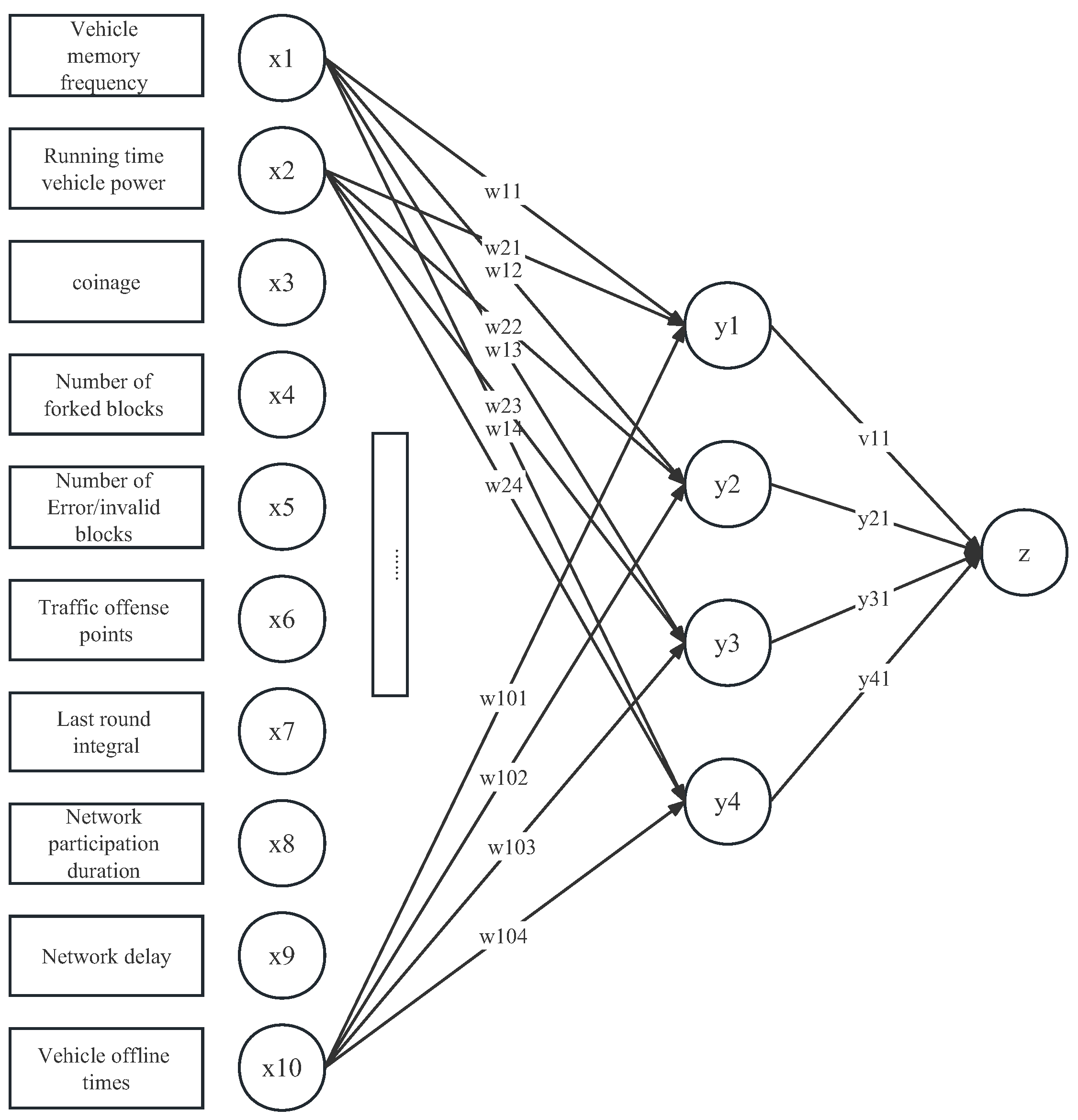
For the indicators in the integral model, many studies put forward many neural network models to solve it. We selected the most representative BP algorithm to our integral model [32]. The structure diagram of BP neural network model in AI-PoV is shown in Figure 3.
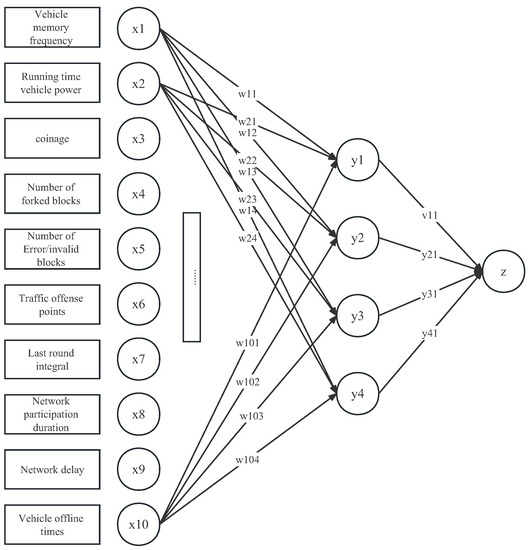
Figure 3.
BP neural network model in AI-PoV.
After all indicators are determined, this paper hopes to determine the vehicle integral after consensus according to these indicators [33]. Different indicators have different impact factors on the results. At this time, BP neural network can be used to conduct error analysis between its own results and standard results through its own training, and then modify the weight value to know some rules, and obtain the result closest to the expected output value at the given input value. At present, the input layer is the secondary index in the integral model, that is, ; the hidden layer corresponds to the primary index, which is ; The output layer corresponds to the integration result . The vector represents the weight between the input layer and the hidden layer, and the vector .
There are two types of input data: discrete data and normally distributed data. For discrete data, most of the integrals will increase or decrease by 1 as the index increases one cycle. Only the error or invalid block provided has a greater impact, which is twice that of other indicators. As a result, its weight is large. Once you have a Byzantine node doing evil, it is going to have an important effect on the final integral. To show the different degrees of influence of different secondary indexes on the results, we quantified the input data [34]. The quantization results of discrete data are shown in Table 4.

Table 4.
Quantitative results of discrete indicators.
Based on the following reasons, some initial input data are normalized in this paper: (1) To avoid some numerical problems leading to deviation of results; (2) improve the speed of convergence, namely training efficiency; (3) data quantization is needed to unify evaluation standards; (4) in BP, sigmoid function is often used as transfer function, and normalization can prevent neuron output saturation caused by excessive net input absolute value. Since the integral may be negative, the data are normalized to [−1,1]. The normalization of discrete data is shown in Equation (1).
where v is the value before normalization, is the minimum value of an attribute, is its maximum value, is the mean value, and is the normalized result.
The non-discrete data need to be normalized and converted into values distributed at (0,1) through the normal distribution function. The normal distribution function is denoted as , and , is set.
So far, the data preprocessing stage has been completed, and then the forward propagation of data and the backpropagation of errors are carried out to learn the weights of each index. In forward propagation, the input signal is transmitted backward from the input layer to the output layer through the hidden layer, and the output signal is generated here. If the error exceeds a certain range with the expected result, the error signal backpropagation process is started: In the process of backpropagation of error signals, the error signals propagate forward successively from the output layer, and the weights between ends are corrected according to the error feedback. The above process will lead to the actual output constantly approaching the expected output [35]. Specific steps and relevant formulas are as follows:
- Initialization of weights. We assign the initial weights w and v as random numbers;
- Input the pre-processed data successively to obtain the hidden layer results, as shown in Equation (3). is the output value of the hidden layer, is the weight value of the input layer to the hidden layer, and is the input value of the input layer. In Equation (4), is the activation function. In order to add nonlinear factors so that the results can approximate arbitrarily complex functions, we use the activation function, which facilitates the control of the hidden layer output range at [−1,1];
- Input the data of the hidden layer successively to obtain the results of the output layer. is the output value of the output layer, is the weight value of the hidden layer to the output layer, and is the input value of the hidden layer;
- Calculate the weight of the backpropagation error adjustment weight w and v;where stands for learning efficiency and is a constant.
- Calculate the cell result of the output layer again according to the new weight, if or reach the maximum number of learning times, then Stop training, or move on to step 2.
4.2. Informer in the Classification Model
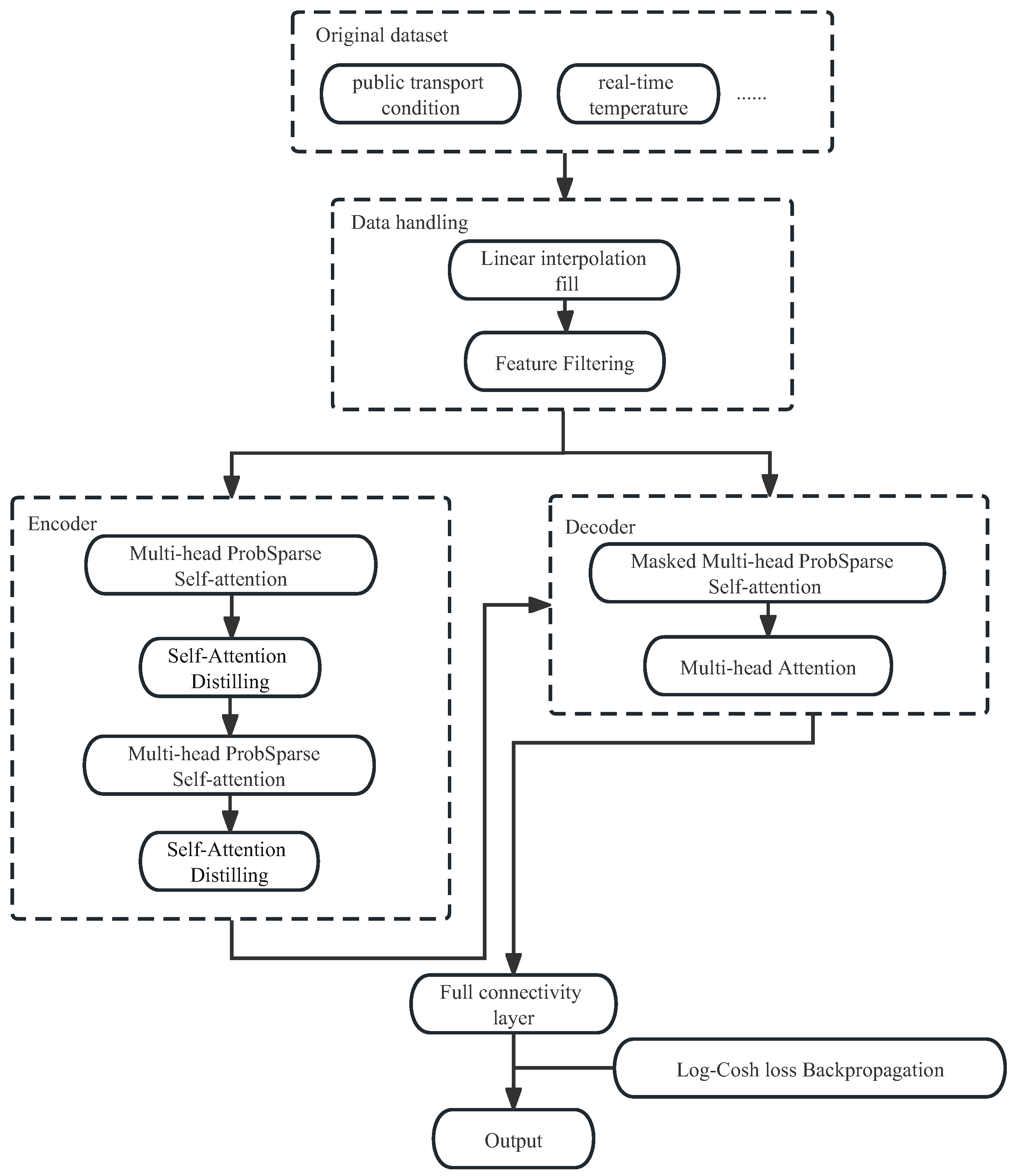
To better classify vehicles, we predict the online situation of vehicles to ensure that the selected primary node vehicles avoid dropping off. For vehicle online state prediction, a lightweight model Informer is adopted [36]. Informer is a supervised learning model based on attention mechanism, which is composed of an encoder and a decoder. The encoder is used to obtain the long-term dependence of the long sequence input, and the decoder can further realize the sequence prediction. The structure diagram of Informer model in AI-PoV is shown in Figure 4.
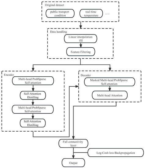
Figure 4.
Informer model in AI-PoV flow chart.
The main content of model input is the influence factor of the first t moments after standardization , because the features of large variance will greatly affect the convergence and accuracy of the model, we conducted standard deviation standardization on the data [37].
where is the standard of original data; x is the original data; as the original data of the mean; z is the standardized data.
The prediction process first carries out feature processing on the original data set and then inputs the processed feature sequence into Informer’s encoding and decoding architecture to capture the long-term correlation between input and output. Finally, the prediction result is obtained through the full connection layer . After calculating the loss function of the output prediction result, the inverse gradient propagation is carried out to optimize the model continuously [38]. In regression problems, the loss function we commonly use is the MSE (Mean Square Error) function. The MSE function quantifies the error of the model by squaring the error in a way that can make the model very sensitive to outliers in the data. There are many chance conditions in the use of vehicles, and our data will have more outliers for which the MSE function is not suitable. Therefore, we trained the Informer model using the Log-Cosh loss function, which is more robust to outliers. These two loss functions are represented as Equation (8) below.
where is the true value and is the predicted value.
5. Performance Evaluation
To verify the effectiveness of the AI-PoV, this section shows a comparative experiment. First, we compare the informer prediction ability in vehicle online duration. Secondly, we compare the AI-PoV with PoW and other classical consensus algorithms in the vehicle-based methods.
5.1. Experiment Environment
The energy consumed in the implementation of the consensus algorithm is measured in a stand-alone environment. The experimental hardware environment is shown in Table 5.

Table 5.
The experiment hardware workbench.
The computer simulates the startup of multiple nodes on the command line by modifying the port number. Take two nodes as an example. Node information is shown in Table 6. Power meter sets the sampling interval to 1 s and measures the energy consumption of all nodes during the algorithm by measuring the total power of the cluster.

Table 6.
Node information.
The experimental software environment is shown in Table 7. The written framework is packaged into an executable jar package through Maven install. The port number and service port number of the jar package are different for different nodes and are placed on the local machine. Run the following command to run node1: java -jar blockchain01.jar. In this case, node1 can generate blocks. Then run node2 node, which can connect to node1. node1 propagates block or blockchain information to node2, and the two nodes reach an agreement. The process of starting a new node is similar. The data analysis system of the electric detector runs in the machine, and its function is to save the indicators measured by the power meter and export them in xls and other formats.

Table 7.
The experiment software workbench.
5.2. Online Duration Prediction Based on Informer
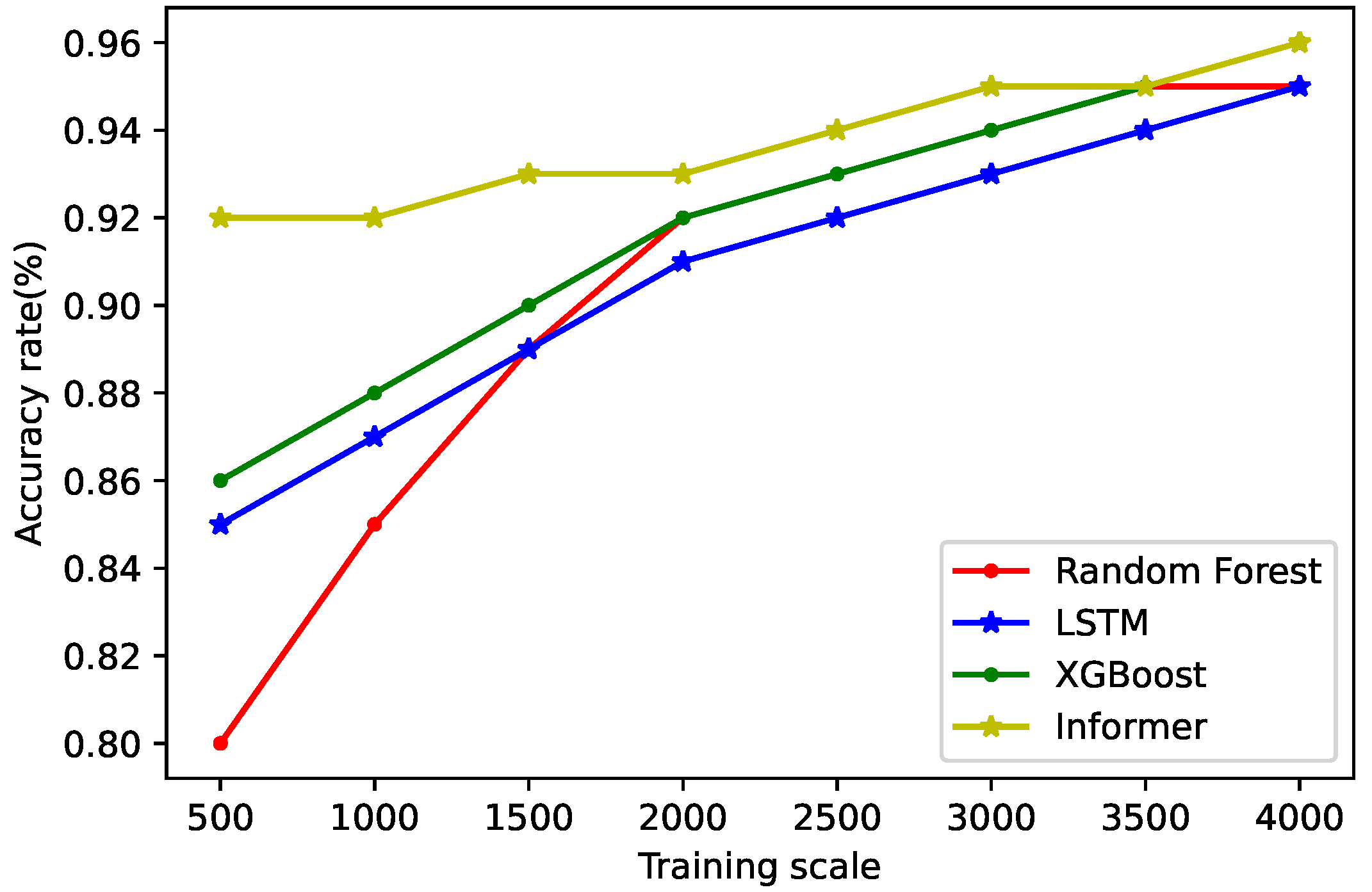
In collaborative IoV, the accuracy and convenience of vehicle online time prediction directly affect the accuracy and efficiency of vehicle interconnection. In this section, we compare the informer used in this study and the commonly used prediction methods (Random Forest, LSTM, and XGBoost) in terms of prediction accuracy and prediction time.
Our data comes from the Weather Big Data interface service provided by China Meteorological Data Network (http://www.nmic.cn/Market/index.html, accessed on 1 July 2019). We selected data recorded at weather stations in Shenyang and Dalian, two cities in Liaoning Province, China, to obtain meteorological data for April 2019–June 2019, including temperature, precipitation, and other data. Vehicle usage data were obtained from vehicle research in 2019 of Liaoning highway in China, including vehicle life, vehicle violation, vehicle usage time, and other data. Firstly, the data are pre-processed, the data of temperature and precipitation are recorded every 0.5 h to obtain a total of 4368 sets of data, and the time periods of vehicle use are divided to obtain a total of 4687 sets of data. The two datasets are matched for time periods, and for the missing parts in data collection, we used a linear interpolation method to fill in.
We implemented Informer, Random Forest, LSTM, and XGBoost using the PyTorch deep learning framework, dividing the data into two groups, 5000 for training and 1687 for testing. The parameters of the model are set as follows: the initial learning rate of Informer is set to 0.0001 and the weight matrix is randomly initialized, which uses Log-Cosh as the loss function for model training, the batch size is set to 32, and the number of iterations is 8; the max_features of Random Forest is set to 0.8, n_estimators is set to 69, max_depth is set to 8, LSTM is set to 2 layers, the number of neurons is set to 32 in layer 1 and 160 in layer 2 by super optimization; n_estimators is set to 1000, Subsample is set to 0.8, colsample_bytree is set to 0.8, and learning_rate is set to 0.8. is set to 0.8 and learning_rate is set to 0.1.
We conducted four comparative experiments, and the specific experimental results are shown in Figure 5 and Figure 6. We define the criterion for evaluating model complexity as . where is the minimum storage space required by the model, is the minimum memory required for the model to run and is the mean of the running time; a, b, and c are the coefficients that normalize their corresponding metrics.
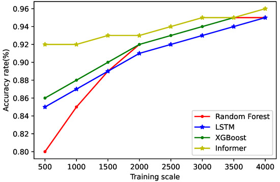
Figure 5.
Comparison of prediction accuracy.
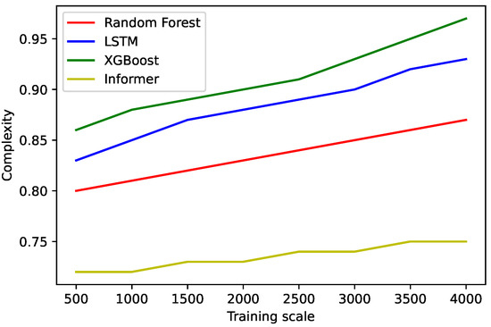
Figure 6.
Comparison of the complexity.
5.3. Performance Comparison of AI-PoV
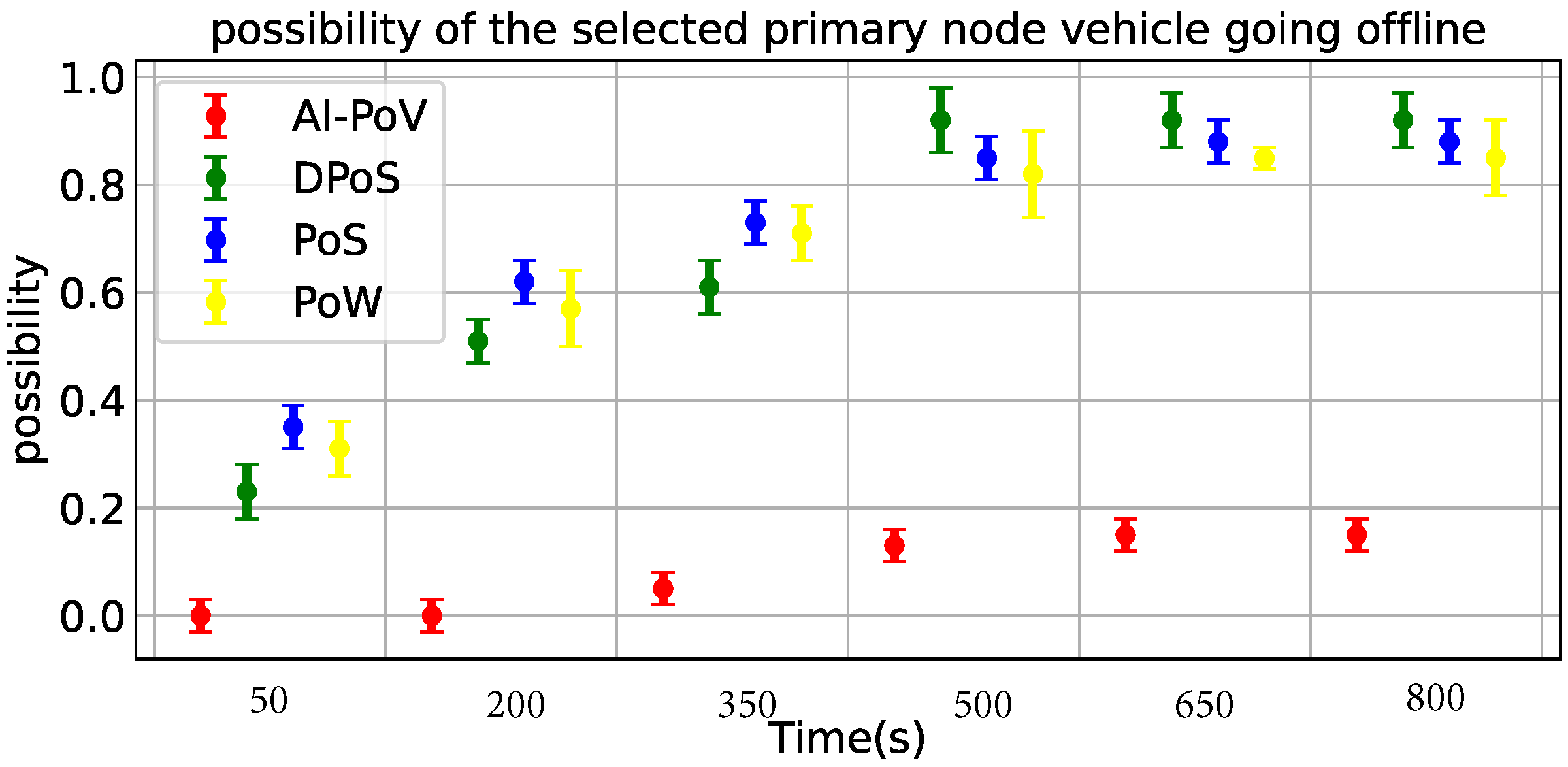
AI-PoV is more suitable for collaborative IoV because it considers vehicle features. On the one hand, we eliminate the possibility of selecting the vehicle that is about to come off the line as the primary node vehicle. In this section, we use computers to simulate vehicles as a node in the blockchain.We first compared AI-PoV algorithm and PoW, PoS and DPoS algorithm respectively in the possibility of the selected primary node vehicle disconnection within 50 s, 200 s, 350 s, 500 s, 650 s, and 800 s. On the other hand, AI-PoV algorithm reduces the time delay caused by a large number of calculations, thus reducing the energy consumption of collaborative IoV. We compare the delay and energy consumption of AI-PoV algorithm and three other classical algorithms.
The tools used in the data sources of the pre-experimental simulation include the traffic flow simulation tool VanetMobiSim (version 1.1) and the network simulation tool OPNET (version 14.5). In this experiment, VanetMobiSim tool is used to generate simulated roads in two areas, which are 4000 m and the number of vehicles is 800–1000. In the simulation experiment in Section 5.3.2, data sets of 7:30 and 16:30 in these two areas were selected, respectively. The trajectory of the vehicle is generated by VanetMobiSim and then imported into the OPNET simulation environment of the mobile node to simulate the communication between vehicles.
5.3.1. The Possibility of Primary Node Vehicle Offline
In the four groups of data generated by VanetMobiSim tool in two areas at different times, we selected 100 node vehicles proportionally to analyze the possibility of vehicle disconnection.
As shown in Figure 7, the experimental results show that the possibility of the main node vehicle selected by AI-PoV going offline is zero within 50 s and 200 s. In the other three methods, the possibility of primary node vehicle offline is about 30% and 50%. In 350 s to 800 s, the probability of the primary node selected by the AI-PoV going offline is 5% to 10%. In the other three methods, the possibility of primary node vehicle offline is 70% to 85%. AI-PoV greatly reduces the risk of primary node vehicle offline and avoids the communication cost of re-selecting primary node vehicle.
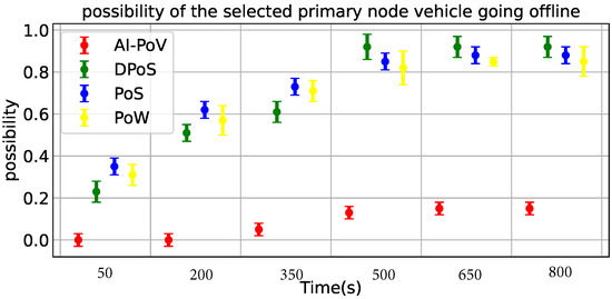
Figure 7.
Comparison of the possibility of the selected primary node vehicle going offline within 50 s, 200 s, 350 s, 500 s, 650 s, and 800 s (compared with PoW, PoS, and DPoS).
5.3.2. Delay and Energy Consumption
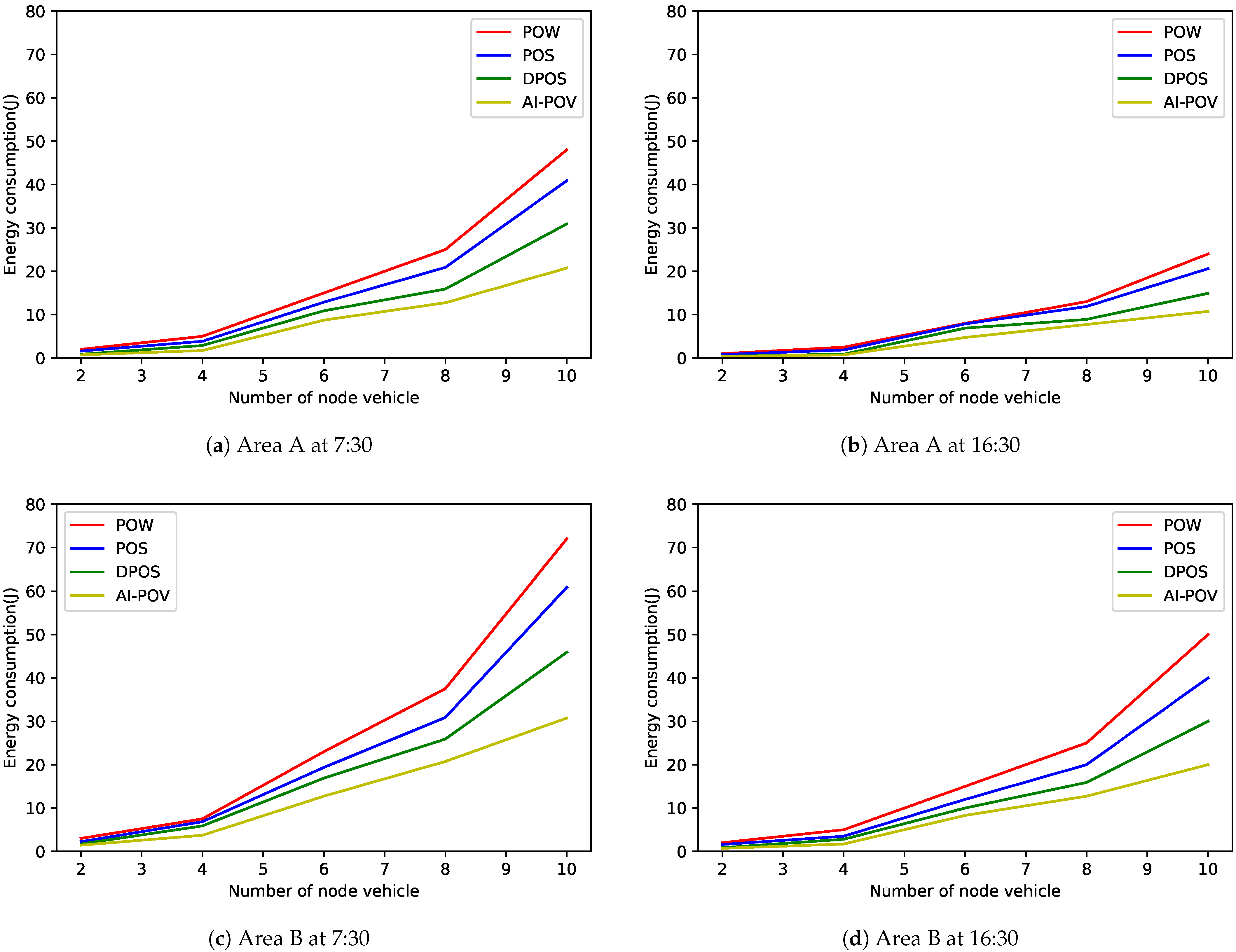
The energy consumption of the system is positively correlated with the computational complexity, that is, in collaborative networking of vehicles, the energy consumption is positively correlated with the latency.
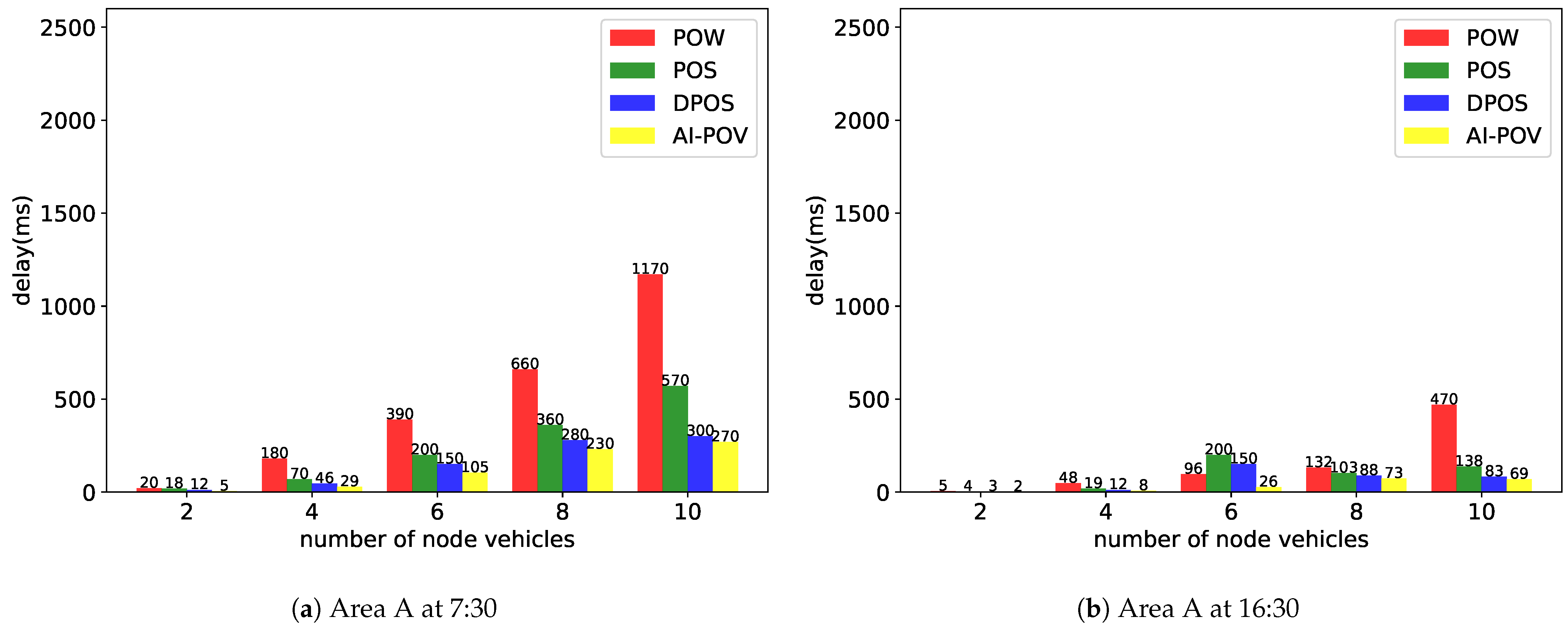
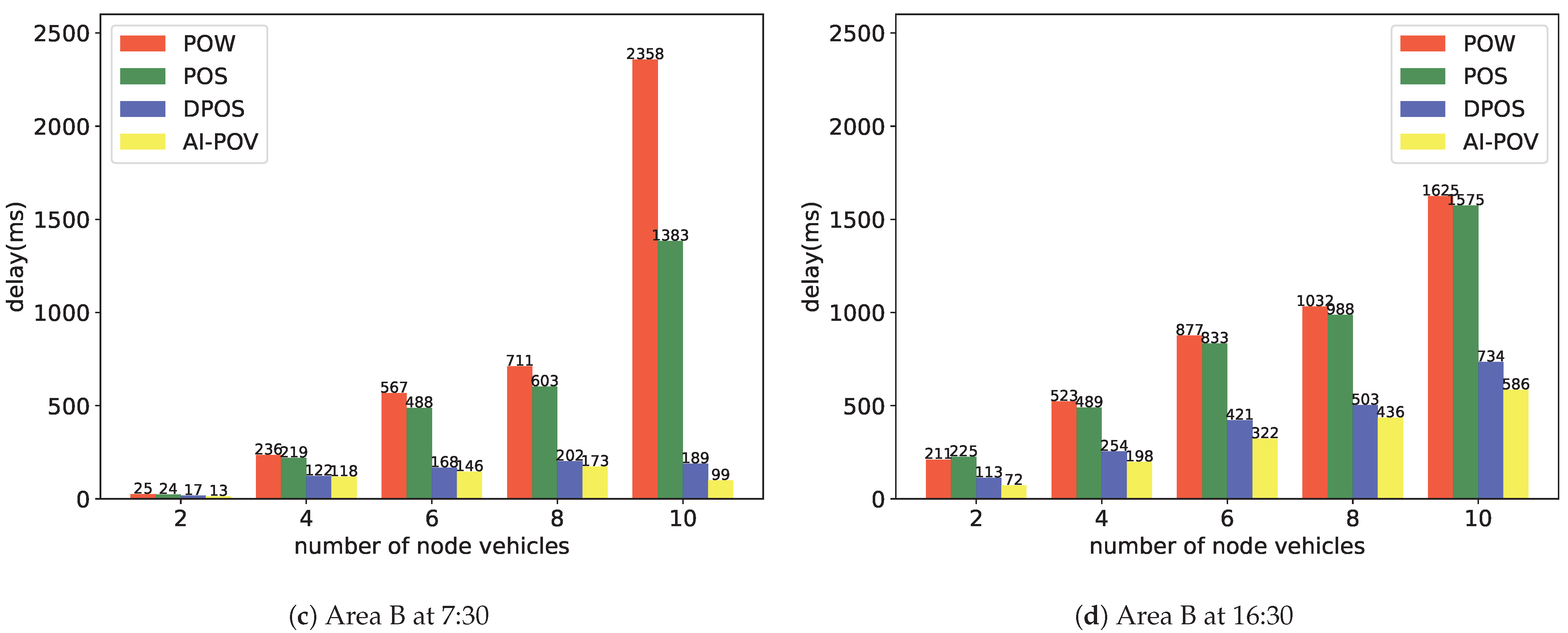
As shown in Figure 8, the more nodes there are, the more delay the collaborative IoV system will generate. When the number of nodes is the same, AI-PoV saves nearly half of the time delay compared with other algorithms and nearly half of the computing energy.
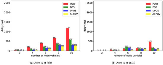
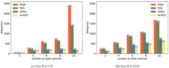
Figure 8.
Comparison of the complexity.
As shown in Figure 8 and Figure 9, compared with the three most widely used consensus algorithms, AI-PoV solves the immediate off-line problem of primary node vehicles and realizes the challenge of considering vehicle features in collaborative IoV. At the same time, it reduces the system delay in the blockchain environment, reduces the system energy consumption, and has better applicability for collaborative IoV.
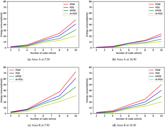
Figure 9.
Comparison of energy consumption of four consensus algorithms.
6. Conclusions
We want to solve the problem of communication cost caused by asymmetric IoV structure through the cooperation between vehicles in the blockchain environment. The implementation of vehicle-based collaborative IoV is closely related to avoiding off-line of primary node vehicle and reducing delay. Therefore, it is a big challenge to reduce the delay while avoiding the off-line of the primary node vehicle. To solve it, this paper proposed a novel consensus algorithm. Specifically, we have used blockchain as a prototype and established indicators based on vehicles, proposed integral and rating models, and used the BP algorithm and the Informer model to solve the problem. After scoring the vehicles, classification is performed, and further vehicle selection is done through offline prediction to select the optimal master node for broadcasting and proposing. Experimental results show that, compared with existing consensus algorithms, the master node selected by AI-PoV has high efficiency, high fault tolerance, avoiding the vehicle dropout of the master node, and reducing the communication delay between vehicles. Through the consensus among vehicles, it can replace part of the data sharing of the traditional centralized IoV and alleviate the negative impact of communication delay caused by its asymmetric network structure. In the future, we plan to expand our work in three main areas. Firstly, we broaden the vehicle indicators referenced by the Integral model through the extensive collection and feature screening of vehicle information. Secondly, we aim to improve the accuracy of the prediction by optimizing the Informer model in the Classification model.
Author Contributions
Conceptualization, C.S. and D.L.; methodology, C.S. and D.L.; software, C.S.; validation, C.S. and D.L.; formal analysis, J.S. and B.W.; investigation, C.S.; resources, B.W.; data curation, D.L.; writing—original draft preparation, C.S.; writing—review and editing, C.S. and D.L.; visualization, C.S. and D.L.; supervision, B.W.; project administration, D.L.; funding acquisition, J.S. All authors have read and agreed to the published version of the manuscript.
Funding
This research was funded by “Liaoning Provincial Transportation Investment Group Scientific Research Project (Differentiation)”.
Data Availability Statement
The authors confirm that the data supporting the findings of this study are available within the article.
Conflicts of Interest
The authors declare no conflict of interest.
References
- Zhang, J.; Wang, F.Y.; Wang, K.; Lin, W.H.; Xu, X.; Chen, C. Data-Driven Intelligent Transportation Systems: A Survey. IEEE Trans. Intell. Transp. Syst. 2011, 12, 1624–1639. [Google Scholar] [CrossRef]
- Chen, K.; Zhang, S.; Li, Z.; Zhang, Y.; Deng, Q.; Ray, S.; Jin, Y. Internet-of-Things Security and Vulnerabilities: Taxonomy, Challenges, and Practice. J. Hardw. Syst. Secur. 2018, 2, 97–110. [Google Scholar] [CrossRef]
- Yang, F.; Wang, S.; Li, J.; Liu, Z.; Sun, Q. An Overview of Internet of Vehicles. China Commun. 2014, 11, 1–15. [Google Scholar] [CrossRef]
- Kaiwartya, O.; Abdullah, A.H.; Cao, Y.; Altameem, A.; Prasad, M.; Lin, C.T.; Liu, X. Internet of Vehicles: Motivation, Layered Architecture, Network Model, Challenges, and Future Aspects. IEEE Access 2016, 4, 5356–5373. [Google Scholar] [CrossRef]
- Jia, X.; Song, X.; Sohail, M. Effective Consensus-Based Distributed Auction Scheme for Secure Data Sharing in Internet of Things. Symmetry 2022, 14, 1664. [Google Scholar] [CrossRef]
- Qu, Y.; Xiong, N. RFH: A Resilient, Fault-Tolerant and High-Efficient Replication Algorithm for Distributed Cloud Storage. In Proceedings of the 2012 41st International Conference on Parallel Processing, Pittsburgh, PA, USA, 10–13 September 2012; pp. 520–529. [Google Scholar] [CrossRef]
- Jiang, T.; Fang, H.; Wang, H. Blockchain-Based Internet of Vehicles: Distributed Network Architecture and Performance Analysis. IEEE Internet Things J. 2019, 6, 4640–4649. [Google Scholar] [CrossRef]
- Wang, C.; Cheng, X.; Li, J.; He, Y.; Xiao, K. A Survey: Applications of Blockchain in the Internet of Vehicles. EURASIP J. Wirel. Commun. Netw. 2021, 2021, 1–16. [Google Scholar] [CrossRef]
- Abdi, A.I.; Eassa, F.E.; Jambi, K.; Almarhabi, K.; AL-Ghamdi, A.S.A.M. Blockchain Platforms and Access Control Classification for IoT Systems. Symmetry 2020, 12, 1663. [Google Scholar] [CrossRef]
- Bada, A.O.; Damianou, A.; Angelopoulos, C.M.; Katos, V. Towards a Green Blockchain: A Review of Consensus Mechanisms and Their Energy Consumption. In Proceedings of the 2021 17th International Conference on Distributed Computing in Sensor Systems, Los Angeles, CA, USA, 14–16 July 2021; pp. 503–511. [Google Scholar] [CrossRef]
- Ismail, L.; Materwala, H. A Review of Blockchain Architecture and Consensus Protocols: Use Cases, Challenges, and Solutions. Symmetry 2019, 11, 1198. [Google Scholar] [CrossRef]
- Namasudra, S.; Crespo, R.G.; Kumar, S. Introduction to the Special Section on Advances of Machine Learning in Cybersecurity (VSI-mlsec). Comput. Electr. Eng. 2022, 100, 108048. [Google Scholar] [CrossRef]
- Fan, B.; Zhang, Y.; Chen, Y.; Meng, L. Intelligent Vehicle Lateral Control Based on Radial Basis Function Neural Network Sliding Mode Controller. CAAI Trans. Intell. Technol. 2022, 7, 455–468. [Google Scholar] [CrossRef]
- Yang, M. Research on Vehicle Automatic Driving Target Perception Technology Based on Improved MSRPN Algorithm. J. Comput. Cogn. Eng. 2022, 1, 147–151. [Google Scholar] [CrossRef]
- Elia, R.; Plastiras, G.; Pettemeridou, E.; Savva, A.; Theocharides, T. A Real-world Data Collection Framework for a Fused Dataset Creation for Joint Human and Remotely Operated Vehicle Monitoring and Anomalous Command Detection. CAAI Trans. Intell. Technol. 2022, 7, 432–445. [Google Scholar] [CrossRef]
- Wang, T.; Ai, S.; Cao, J.; Zhao, Y. A Blockchain-Based Distributed Computational Resource Trading Strategy for Internet of Things Considering Multiple Preferences. Symmetry 2023, 15, 808. [Google Scholar] [CrossRef]
- Cui, T.; Yang, R.; Fang, C.; Yu, S. Deep Reinforcement Learning-Based Resource Allocation for Content Distribution in IoT-Edge-Cloud Computing Environments. Symmetry 2023, 15, 217. [Google Scholar] [CrossRef]
- Tang, L.; Tang, B.; Tang, L.; Guo, F.; Zhang, J. Reliable Mobile Edge Service Offloading Based on P2P Distributed Networks. Symmetry 2020, 12, 821. [Google Scholar] [CrossRef]
- Nakamoto, S. Bitcoin: A Peer-to-Peer Electronic Cash System. Decentralized Business Review. 2008, p. 21260. Available online: https://bitcoin.org/en/bitcoin-paper (accessed on 8 April 2023).
- Cao, B.; Zhang, Z.; Feng, D.; Zhang, S.; Zhang, L.; Peng, M.; Li, Y. Performance Analysis and Comparison of PoW, PoS and DAG Based Blockchains. Digit. Commun. Netw. 2020, 6, 480–485. [Google Scholar] [CrossRef]
- Li, C.; Palanisamy, B. Comparison of Decentralization in Dpos and Pow Blockchains. In Proceedings of the Blockchain—ICBC, Honolulu, HI, USA, 18–20 September 2020; Springer: Berlin/Heidelberg, Germany, 2020; pp. 18–32. [Google Scholar] [CrossRef]
- Zhou, X.; Yang, X.; Ma, J.; Kevin, I.; Wang, K. Energy-Efficient Smart Routing Based on Link Correlation Mining for Wireless Edge Computing in Iot. IEEE Internet Things J. 2021, 9, 14988–14997. [Google Scholar] [CrossRef]
- Yang, Z.; Yang, K.; Lei, L.; Zheng, K.; Leung, V.C. Blockchain-Based Decentralized Trust Management in Vehicular Networks. IEEE Internet Things J. 2018, 6, 1495–1505. [Google Scholar] [CrossRef]
- Liu, X.; Huang, H.; Xiao, F.; Ma, Z. A Blockchain-Based Trust Management with Conditional Privacy-Preserving Announcement Scheme for VANETs. IEEE Internet Things J. 2019, 7, 4101–4112. [Google Scholar] [CrossRef]
- Kang, J.; Xiong, Z.; Niyato, D.; Ye, D.; Kim, D.I.; Zhao, J. Toward Secure Blockchain-Enabled Internet of Vehicles: Optimizing Consensus Management Using Reputation and Contract Theory. IEEE Trans. Veh. Technol. 2019, 68, 2906–2920. [Google Scholar] [CrossRef]
- Gao, S.; Yu, T.; Zhu, J.; Cai, W. T-PBFT: An EigenTrust-based Practical Byzantine Fault Tolerance Consensus Algorithm. China Commun. 2019, 16, 111–123. [Google Scholar] [CrossRef]
- Xu, X.; Gu, J.; Yan, H.; Liu, W.; Qi, L.; Zhou, X. Reputation-Aware Supplier Assessment for Blockchain-Enabled Supply Chain in Industry 4.0. IEEE Trans. Ind. Inform. 2022, 19, 5485–5494. [Google Scholar] [CrossRef]
- Huang, J.; Kong, L.; Chen, G.; Wu, M.Y.; Liu, X.; Zeng, P. Towards Secure Industrial IoT: Blockchain System with Credit-Based Consensus Mechanism. IEEE Trans. Ind. Inform. 2019, 15, 3680–3689. [Google Scholar] [CrossRef]
- Guo, C.; Zhong, Z.; Zhang, Z.; Song, J. NeurstrucEnergy: A Bi-Directional GNN Model for Energy Prediction of Neural Networks in IoT. Digit. Commun. Netw. 2022; in press. [Google Scholar] [CrossRef]
- Zhou, X.; Hu, Y.; Wu, J.; Liang, W.; Ma, J.; Jin, Q. Distribution Bias Aware Collaborative Generative Adversarial Network for Imbalanced Deep Learning in Industrial IoT. IEEE Trans. Ind. Inform. 2022, 19, 570–580. [Google Scholar] [CrossRef]
- Raman, R.; Gupta, N.; Jeppu, Y. Framework for Formal Verification of Machine Learning Based Complex System-of-Systems. Insight 2023, 26, 91–102. [Google Scholar] [CrossRef]
- Li, J.; Cheng, J.H.; Shi, J.Y.; Huang, F. Brief Introduction of Back Propagation (BP) Neural Network Algorithm and Its Improvement. In Proceedings of the Advances in Intelligent and Soft Computing, Delhi, India, 25–27 May 2012; Springer: Berlin/Heidelberg, Germany, 2012; Volume 169, pp. 553–558. [Google Scholar] [CrossRef]
- Liu, L.; Liu, D.; Sun, Q.; Li, H.; Wennersten, R. Forecasting Power Output of Photovoltaic System Using a BP Network Method. Energy Procedia 2017, 142, 780–786. [Google Scholar] [CrossRef]
- Krichen, M.; Mihoub, A.; Alzahrani, M.Y.; Adoni, W.Y.H.; Nahhal, T. Are Formal Methods Applicable To Machine Learning And Artificial Intelligence? In Proceedings of the 2022 2nd International Conference of Smart Systems and Emerging Technologies (SMARTTECH), Riyadh, Saudi Arabia, 9–12 May 2022; pp. 48–53. [Google Scholar] [CrossRef]
- Vasko, F.J.; Lu, Y.; McNally, B. A Simple Methodology That Efficiently Generates All Optimal Spanning Trees for the Cable-Trench Problem. J. Comput. Cogn. Eng. 2022, 1, 13–20. [Google Scholar] [CrossRef]
- Zhou, H.; Zhang, S.; Peng, J.; Zhang, S.; Li, J.; Xiong, H.; Zhang, W. Informer: Beyond Efficient Transformer for Long Sequence Time-Series Forecasting. In Proceedings of the AAAI Conference on Artificial Intelligence, Virtual, 2–9 February 2021; Volume 35, pp. 11106–11115. [Google Scholar] [CrossRef]
- Devi, D.; Namasudra, S.; Kadry, S. A Boosting-Aided Adaptive Cluster-Based Undersampling Approach for Treatment of Class Imbalance Problem. Int. J. Data Warehous. Min. 2020, 16, 60–86. [Google Scholar] [CrossRef]
- Malviya, S.; Kumar, P.; Namasudra, S.; Tiwary, U.S. Experience Replay-based Deep Reinforcement Learning for Dialogue Management Optimisation. ACM Trans. Asian Low-Resour. Lang. Inf. Process. 2022, 3539223. [Google Scholar] [CrossRef]
Disclaimer/Publisher’s Note: The statements, opinions and data contained in all publications are solely those of the individual author(s) and contributor(s) and not of MDPI and/or the editor(s). MDPI and/or the editor(s) disclaim responsibility for any injury to people or property resulting from any ideas, methods, instructions or products referred to in the content. |
© 2023 by the authors. Licensee MDPI, Basel, Switzerland. This article is an open access article distributed under the terms and conditions of the Creative Commons Attribution (CC BY) license (https://creativecommons.org/licenses/by/4.0/).

